Design and Tuning of an Evolutionary Multiobjective ... - Eldorado

Design and Tuning of an Evolutionary Multiobjective Optimisation Algorithm

Dissertation zur Erlangung des Grades eines

D OKTORS DER N ATURWISSENSCHAFTEN ¨ Dortmund der Technischen Universitat am Fachbereich Informatik von

Boris Naujoks Dortmund

2011

2

Tag der mundlichen Prufung: ¨ ¨

¨ 2011 29. Marz

Dekan:

Prof. Dr. P. Buchholz

Gutachter:

Prof. Dr. G. Rudolph, TU Dortmund Prof. Dr. Y. Jin, University of Surrey, GB

3

Contents 1 Introduction 1.1 Preliminaries . . . . . . . . . . . . . . . . . . . . . . . . . . . 1.2 Example and Fundamentals . . . . . . . . . . . . . . . . . . . 1.3 Overview . . . . . . . . . . . . . . . . . . . . . . . . . . . . . 1.3.1 The basic S -Metric Selection - EMOA . . . . . . . . . . 1.3.2 Diversity Preservation in Decision and Objective Space 1.3.3 Many-Objective Optimisation . . . . . . . . . . . . . . 1.3.4 Stopping Criteria for EMOA . . . . . . . . . . . . . . . 1.3.5 Sequential Parameter Optimisation for MCO . . . . . .

. . . . . . . .

. . . . . . . .

. . . . . . . .

. . . . . . . .

. . . . . . . .

. . . . . . . .

. . . . . . . .

. . . . . . . .

. . . . . . . .

. . . . . . . .

. . . . . . . .

. . . . . . . .

5 5 6 8 9 10 10 10 11

2 The basic S -Metric Selection - EMOA 2.1 An EMO Algorithm Using the Hypervolume Measure as Selection Criterion . . . . . . 2.1.1 Introduction . . . . . . . . . . . . . . . . . . . . . . . . . . . . . . . . . . . . 2.1.2 The Hypervolume Measure . . . . . . . . . . . . . . . . . . . . . . . . . . . 2.1.3 The Algorithm . . . . . . . . . . . . . . . . . . . . . . . . . . . . . . . . . . 2.1.4 Test Problems . . . . . . . . . . . . . . . . . . . . . . . . . . . . . . . . . . 2.1.5 Design Optimization . . . . . . . . . . . . . . . . . . . . . . . . . . . . . . . 2.1.6 Summary and Outlook . . . . . . . . . . . . . . . . . . . . . . . . . . . . . . 2.2 Multi-objective Optimisation using S -metric Selection: Application to three-dimensional Solution Spaces . . . . . . . . . . . . . . . . . . . . . . . . . . . . . . . . . . . . . 2.2.1 Introduction . . . . . . . . . . . . . . . . . . . . . . . . . . . . . . . . . . . . 2.2.2 Previous Work . . . . . . . . . . . . . . . . . . . . . . . . . . . . . . . . . . 2.2.3 Selection Criteria and EMOA framework . . . . . . . . . . . . . . . . . . . . 2.2.4 Results on Test Problems . . . . . . . . . . . . . . . . . . . . . . . . . . . . 2.2.5 Design Optimisation . . . . . . . . . . . . . . . . . . . . . . . . . . . . . . . 2.2.6 Summary and Outlook . . . . . . . . . . . . . . . . . . . . . . . . . . . . . .

13 16 16 17 18 21 24 28

3 Diversity Preservation in Decision and Objective Space 3.1 Pareto Set and EMOA Behavior for Simple Multimodal Multiobjective Functions 3.1.1 Introduction . . . . . . . . . . . . . . . . . . . . . . . . . . . . . . . . . 3.1.2 Aims and Methods . . . . . . . . . . . . . . . . . . . . . . . . . . . . . 3.1.3 A Simple Test Problem: TWO-ON-ONE . . . . . . . . . . . . . . . . . . 3.1.4 Experimental Investigation of Pareto Sets . . . . . . . . . . . . . . . . . 3.1.5 Analytical Derivation of Pareto Sets . . . . . . . . . . . . . . . . . . . . 3.1.6 Behavior of EMOAs on TWO-ON-ONE . . . . . . . . . . . . . . . . . . 3.1.7 Summary and Outlook . . . . . . . . . . . . . . . . . . . . . . . . . . . 3.2 Capabilities of EMOA to Detect and Preserve Equivalent Pareto Subsets . . . . 3.2.1 Introduction . . . . . . . . . . . . . . . . . . . . . . . . . . . . . . . . . 3.2.2 Aims and Methods . . . . . . . . . . . . . . . . . . . . . . . . . . . . .

43 45 45 46 46 47 50 51 53 54 54 55

. . . . . . . . . . .

. . . . . . . . . . .

. . . . . . . . . . .

29 29 30 32 36 39 41

4

3.2.3 3.2.4 3.2.5 3.2.6

A test-problem class: SYM-PART . . . . . . . . . Evaluation of Standard EMOA on SYM-PART . . . A Multistart Approach for Pareto Subset Detection Conclusions and Future Work . . . . . . . . . . .

. . . .

. . . .

. . . .

. . . .

. . . .

. . . .

. . . .

. . . .

. . . .

. . . .

. . . .

. . . .

. . . .

. . . .

. . . .

56 60 65 67

4 Many-Objective Optimisation 4.1 Pareto-, Aggregation-, and Indicator-based Methods in Many-objective Optimization 4.1.1 Introduction . . . . . . . . . . . . . . . . . . . . . . . . . . . . . . . . . . . 4.1.2 Benchmark Settings . . . . . . . . . . . . . . . . . . . . . . . . . . . . . . 4.1.3 Pareto-based EMOA . . . . . . . . . . . . . . . . . . . . . . . . . . . . . . 4.1.4 Aggregation-based EMOA . . . . . . . . . . . . . . . . . . . . . . . . . . . 4.1.5 Indicator-based EMOA . . . . . . . . . . . . . . . . . . . . . . . . . . . . . 4.1.6 Summary and Outlook . . . . . . . . . . . . . . . . . . . . . . . . . . . . .

. . . . . . .

69 71 71 72 73 77 80 83

5 Stopping Criteria for EMOA 5.1 Online Convergence Detection for Evolutionary Multi-Objective Algorithms Based on Statistical Testing . . . . . . . . . . . . . . . . . . . . . . . . . . . . . . . . . . . . 5.1.1 Introduction . . . . . . . . . . . . . . . . . . . . . . . . . . . . . . . . . . . . 5.1.2 State of the Art . . . . . . . . . . . . . . . . . . . . . . . . . . . . . . . . . . 5.1.3 Online Convergence Detection . . . . . . . . . . . . . . . . . . . . . . . . . 5.1.4 Experiments . . . . . . . . . . . . . . . . . . . . . . . . . . . . . . . . . . . 5.1.5 Conclusion . . . . . . . . . . . . . . . . . . . . . . . . . . . . . . . . . . . . 5.2 Online Convergence Detection for Multiobjective Aerodynamic Applications . . . . . . 5.2.1 Introduction . . . . . . . . . . . . . . . . . . . . . . . . . . . . . . . . . . . . 5.2.2 Online convergence Detection . . . . . . . . . . . . . . . . . . . . . . . . . . 5.2.3 Aerodynamic Applications . . . . . . . . . . . . . . . . . . . . . . . . . . . . 5.2.4 Airfoil Reconstruction Test Case: NACA . . . . . . . . . . . . . . . . . . . . . 5.2.5 Airfoil Pressure Minimization Test Case: RAE . . . . . . . . . . . . . . . . . . 5.2.6 Experiments . . . . . . . . . . . . . . . . . . . . . . . . . . . . . . . . . . . 5.2.7 Summary and Outlook . . . . . . . . . . . . . . . . . . . . . . . . . . . . . .

85 87 87 88 89 93 100 104 104 105 108 108 109 110 120

6 Sequential Parameter Optimisation for EMOA 6.1 Sequential Parameter Optimization for Multi-Objective Problems . . . . . . . . . . . . 6.1.1 Introduction . . . . . . . . . . . . . . . . . . . . . . . . . . . . . . . . . . . . 6.1.2 Sequential Parameter Optimization . . . . . . . . . . . . . . . . . . . . . . . 6.1.3 Experimental Results . . . . . . . . . . . . . . . . . . . . . . . . . . . . . . 6.1.4 Conclusions . . . . . . . . . . . . . . . . . . . . . . . . . . . . . . . . . . . 6.2 Parameter Tuning Boosts Performance of Variation Operators in Multiobjective Optimization . . . . . . . . . . . . . . . . . . . . . . . . . . . . . . . . . . . . . . . . . 6.2.1 Introduction . . . . . . . . . . . . . . . . . . . . . . . . . . . . . . . . . . . . 6.2.2 Preliminaries . . . . . . . . . . . . . . . . . . . . . . . . . . . . . . . . . . . 6.2.3 Experiments . . . . . . . . . . . . . . . . . . . . . . . . . . . . . . . . . . . 6.2.4 DE vs. SBX on CEC 2007 Problems . . . . . . . . . . . . . . . . . . . . . . 6.2.5 Conclusions . . . . . . . . . . . . . . . . . . . . . . . . . . . . . . . . . . .

121 123 123 124 127 137

7 Conclusions and Future Work

149

139 139 140 141 141 146

5

Chapter 1 Introduction The central topic of this thesis is evolutionary multiobjective optimisation (EMO). This term is the link between all the different chapters, one special aspect of EMO is addressed in each chapter. But what does this term mean, what is evolutionary multiobjective optimisation?

1.1 Preliminaries The by far simplest term within EMO is optimisation. At least it is the simplest part to explain. Each of us once tried to improve something, to get better in some kind of sports, improve some language or writing skills, or learn some musical instrument. All these aspects can be expressed as some kind of optimisation. Mathematically, the most essential aspects within optimisation are a set of feasible solutions S ⊂ Rn and a fitness function f (x) expressing the quality of each solution x ∈ S. Presuming this, an optimisation problem is defined by the task to find the solution x∗ ∈ S such as

f (x∗ ) ≤ f (x),

∀x ∈ S

(1.1)

in case of minimisation. The maximisation case is of course defined in an analogous way using ”≥” instead of ”≤” in equation 1.1. Although explaining or defining optimisation is somehow straightforward, optimisation itself or corresponding procedures and algorithms are a large and complex area of research over decades. At one end, there are first and second order derivative methods for single variable functions, which are already taught in calculus in school. For a more experienced reader in the field, these may seem simple again. Of course, many different ends exist and at some other end, there are evolutionary optimisation techniques. These are also called evolutionary algorithms (EA)1 . Such methods try to mimic the natural process of evolution [Fut90] to improve solutions. The most essential driving force for such algorithms is the repetition and the interaction of the variation of existing solutions and a selection process. The interplay of variation and selection leads to an improvement of solutions over a number of generations. This does not hold necessarily, but in most cases EA have proven to be very competitive, reliable, and robust optimisation methods. This particularly holds for black-box optimisation tasks. For more details on different methods and aspects of optimisation, of course focussing on stochastic techniques, we refer to Schwefel [Sch95]. Advisable, introductory textbooks on EA exist from 1

Abbreviations like EMO, EA, EMOA etc. are used in singular as well as their corresponding plural forms throughout this thesis. To this end, EA might mean a special evolutionary algorithm as well as a set or collection of evolutionary algorithms.

6

Chapter 1

DeJong [DeJ06] and Eiben and Smith [ES03]. Moreover, two journals are most important in the core EA field: 1. Evolutionary Computation journal by MIT Press and 2. IEEE Transactions on Evolutionary Computation by IEEE Press. ¨ Introductory articles stem from Back, Hammel, and Schwefel [BHS97] within the IEEE journal as well as by Beyer and Schwefel [BS02] within the Natural Computing journal by Springer. The latter one has an expanded spectrum in contrast to the above more focussing on EA. Evolutionary algorithms receive a remarkable research interest that is also reflected in the numerous contributions to both of its annual major conferences, i.e.

• IEEE Congress on Evolutionary Computation (CEC), an annual event, which is held every two years in conjunction with the major IEEE conferences on neural networks and fuzzy logic as part of the World Congress on Computational Intelligence (WCCI),

• the Genetic and Evolutionary Computation Conference (GECCO), again an annual conference of the ACM SIGEVO. Next to these huge events there are at least two high quality events within the field taking place every two years, i.e.

• Parallel Problem Solving from Nature (PPSN) and • Foundations of Genetic Algorithms (FOGA).

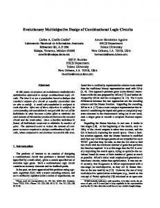
1.2 Example and Fundamentals The missing term in resolving evolutionary multiobjective optimisation is multiobjective, which is possibly the most complex term inside. One task that accompanied me through the past years working and researching in the EMO field was airfoil design. A special task from this field is utilised to introduce multiobjective optimisation. Consider an aircraft wing with a fixed airfoil. For the normal cruising flight conditions, a lift is needed to counterbalance the weight of the whole aircraft. Of course, this lift should be generated with a minimum of drag to save fuel and move the aircraft. This means saving energy and consequently save money as well as protect the environment. However, for special flight conditions, in particular for take-off and landing, other properties of the airfoil are more important. For example, the drag is neglected to receive a certain amount of lift at a special, reduced velocity to provide stable flight characteristics. These conditions obviously yield a trade-off. Different fitness functions can be formulated for the corresponding flight conditions and a good alternative solution for the airfoil is needed. A common approach to handle this multiobjective optimisation problem is to define target airfoils for the corresponding flight conditions and define fitness functions based on the differences of the current airfoil to these target airfoils. Examples for such target airfoils are provided in figure 1.1 with an airfoil featuring a high lift value on the left and one featuring a low drag value on the right hand side. The corresponding fitness functions 1 f1,2 are defined based on the pressure coefficients of the target airfoil maximising lift Cp,target (s), 2 the target airfoil minimising drag Cp,target (s) and the pressure coefficient of the current airfoil Cp (s).

Introduction

7

¨ et al. Figure 1.1: The target airfoils for the NACA redesign test case to be introduced in detail by Back [BHN+ 99] and Naujoks et al. [NWBH02, NHZB02]: NACA 0012 featuring a high lift (left) and NACA 4412 featuring a low drag (right). For a better detection of differences within the designs, the thickness ( y -component in the figures) of the original airfoil is stretched by a factor of 10. Here, s is the airfoil arc-length measured around the airfoil and the resulting fitness functions read

Z f1 :=

1 1 (Cp (s) − Cp,target (s))ds and f2 :=

0

Z

1 2 (Cp (s) − Cp,target (s))ds.

0

The task of evolutionary multiobjective optimisation algorithms (EMOA) within the context above is to determine all solutions that cannot be improved within one aspect without deterioration with respect to the other aspect. Mathematically, this is Pareto-optimisation [Deb01, CVL02], which has become a well established technique for detecting interesting solution candidates for multiobjective optimisation problems. It enables the decision maker to filter efficient solutions and to discover tradeoffs between opposing objectives among these solutions. Provided a set of objective functions f1,...,d : S → R defined on some search space S to be minimised, in Pareto optimisation the aim is to detect the Pareto-optimal set M = {x ∈ S|@x0 ∈ S : x0 ≺ x}. The concept of Pareto dominance relies on a component-wise comparison of vectors. A vector x is said to dominate a vector y (x ≺ y), if and only if f (x) is better than or equal to f (y) in all components, i.e. ∀i ∈ {1, . . . , d} : fi (x) ≤ fi (y) and better than f (y) in at least one component, i.e.

∃j ∈ {1, . . . , d} :

fj (x) < fj (y).

The Pareto-front is the set f (M ) in the objective space. In the airfoil optimisation example from above, all alternative designs, where the lift cannot be increased any further without increasing the drag of the airfoil as well, form this Pareto-front. A unique measure for the quality of a non-dominated set is the hypervolume measure or S metric [ZT98]. In recent years, this measure is utilised within the selection operator in EMOA in order to find a set of well distributed solutions on the Pareto front [ZK04, EBN05, BNE07, IHR07]. Now that the basics of EMO are explained, two textbooks from the last decade have to be mentioned. The first and most well-known one is the book of Deb [Deb01] from 2001. The second book

8

Chapter 1

was written by Coello Coello, Van Veldhuizen, and Lamont in 2002, a new, revised edition was released in 2007 [CVL07]. Next to these introductory books on EMOA in general, Coello Coello and Lamont [CL04] collected different applications of these algorithms and published these in a book again. In addition to major tracks at the annual conference in the evolutionary computation field, there is a special conference series that started back in 2000. It is called the conference on Evolutionary Multi-Criterion Optimization (EMO) and takes place every two years in locations all over the world.

1.3 Overview The work at hand presents approach and enhancements to evolutionary multiobjective optimisation. It is a cumulative work with each paper included co-authored by me. All these papers have been published at different conferences and all have been peer-reviewed, which is the normal procedure within this research field. Based on these conference articles, different journal articles have been published. These are not integrated because I preferred to have the original work in here. Moreover, the journal articles are mostly a condensed version of multiple conference articles and I preferred to have the detailed versions integrated. Due to this thesis being a cumulative work, the nomenclature may change from chapter to chapter, or, but hopefully not, even within one chapter. Moreover, there are different styles of tables, figures etc. throughout the thesis. This is not the normal way a thesis should be presented, but due to the incorporation of different, already published articles. The original layout of tables and figures has intentionally not been changed. Tables and figures may have only been adapted in size to fit adequately in the layout of the thesis. To better distinguish the integrated articles from other text, different fonts have been chosen. Integrated articles are set in LATEX standard font, i.e. Computer Modern Roman, while all other parts are set in Helvetica. Beside this introduction, the work covers six chapters each but the last one focusing on a special aspect of an approach, which is presented here. While the last section concludes this work and presents an outlook to future research tasks, the five chapters in-between present the real scientific work. The main approach to evolutionary multiobjective optimisation described here is an EMOA utilising the hypervolume or S -metric within its selection operator mentioned above (cf. 1.2 on page 7). It is called S -Metric Selection - Evolutionary Multiobjective Optimisation Algorithm (SMS-EMOA). The SMS-EMOA is introduced and analysed in the following chapter. Differences to alternative approaches are worked out and two as well as three dimensional test cases are handled. While the chapters 4 to 6 all present applications of the new approach, extensions, and add-ons, which go beyond the original definition of the algorithm, chapter 3 is different. After having presented the new approach, a more detailed look is taken at the potential and limitations of such Pareto-based approaches in general. To this end, chapter 3 investigates the correlations between Pareto-sets and Pareto-fronts and analyses the basic behaviour of standard EMO algorithms on special test cases. These test cases are built with respect to different correlations of Pareto-sets and Pareto-fronts that might occur in industrial test cases but have been neglected in standard test case definitions for EMOA until now.

Introduction

Chapter 4 comes back to the potential of the SMS-EMOA in contrast to standard EMO algorithms. In the case of three to six dimensions of the objective space, only specialised algorithms are able to provide comparable results to those received with the SMS-EMOA. With increasing objective space dimension, the SMS-EMOA gets more and more superior to well-known, traditional methods. However, the time complexity for the hypervolume calculations should not be neglected. Chapter 5 presents an extension to EMOA in general, that is tested in particular with the SMSEMOA. The Online Convergence Detection (OCD) method provides a stopping criterion that successfully manages the trade-off between wasting computational resources with useless function evaluations and loosing solution quality by stopping an optimisation run too early. The last scientific chapter 6 applies the Sequential Parameter Optimisation (SPO) framework to EMO algorithms in general and the SMS-EMOA in particular. Next to the general applicability of the framework to EMO algorithms, it is utilised to investigate the influence of different variation operators on the performance of the SMS-EMOA. Discussing the influence of variation operators in the last chapter, all aspects of an EMOA algorithm have been handled within this thesis. The possibly most influential one, the selection operator, is the core of the presented new approach. Moreover, the influence of the fitness function has been discussed in chapters 3 (correlations between Pareto-set and Pareto-front) and 4 (many objective optimisation problems). Last, but not least, a very promising new stopping criterion has been proposed (cf. chapter 5). A short overview on the different aspects within each of the following chapters is provided in the following paragraphs.

1.3.1 The basic S -Metric Selection - EMOA This algorithm was first introduced in a joint work with Michael Emmerich and Nicola Beume. The original idea to use the hypervolume as a selection criterion in EMO the chosen way stems from Michael Emmerich. Back in 2004, indicator-based selection was not known, although rather shortly after the first discussions here, a first article on this was published by Zitzler and Kunzli of the Zurich ¨ EMOA group [ZK04]. However, the approach followed there was different in many ways. A basic feature of the SMS-EMOA is its (µ + 1)-selection scheme, that was proposed by me. The main reason to go for such an unusual selection scheme was the high expected runtime for the hypervolume calculations. The presented selection scheme did not solve the problem, but reduced the necessary calculations for the selection to a manageable minimum. Other important design decisions have been taken by the group of authors. While Michael Emmerich provided the first implementation of the algorithm, Nicola and me experimented on already accessible test functions to receive first results. These results were summarised and compared to the results of well-known alternative algorithms in the first paper published at the Evolutionary Multi-Criterion Optimization (EMO) conference in 2005. Since I already had a background in aerodynamic applications, the new algorithm was also applied to a test case from this field. The results received were very promising and have been added to the paper above as well. Another, higher-dimensional and more complex test function from the field of aerodynamics was approached in a follow-up paper [NBE05]. This paper focusses on three dimensional test problems, which have been added to the collection of available test functions. Moreover, it presents a new approach to efficiently calculate three-dimensional hypervolume contributions, which was developed and implemented by Michael Emmerich.

9

10

Chapter 1

1.3.2 Diversity Preservation in Decision and Objective Space Comparing single- and multiobjective evolutionary algorithms, a major difference is the meaning and management of diversity. Within single-objective EA, users try to keep a high diversity in the decision space not to converge to a local optimum too early. Here, Mike Preuss is an expert with a focus on a technique called niching [Pre06]. In multiobjective optimisation, users try to keep a high diversity in the objective space, i.e. a large number of well-spread solutions on the Pareto-front. This way, both species of EA try to keep diversity, but the space where to keep it, decision or objective space, and the methods applied are rather different. Having discussed these differences, Mike Preuss and I agreed that next to keeping diversity in the objective space in EMO, it is use- and helpful to preserve decision space diversity within EMOA as well. A Pareto-optimal solution from a different region of the search space would be much more valuable for a practitioner than only a very small change within one parameter, that he possibly cannot adjust on his machine in reality. Together with Gunter Rudolph we decided to have a more ¨ detailed look on situations that might occur. In two successive years we published two papers that build the core of the corresponding chapter 3.

1.3.3 Many-Objective Optimisation The work of Evan Hughes at the Congress on Evolutionary Computation (CEC) in 2005 mentions the drawbacks of well-known EMO approaches if the number of objectives is increased [Hug05]. This holds, even if the increase is only marginal, i.e. the number of objectives gets larger than three. However, no detailed work focusing on this aspect existed at that time. Hughes himself only compared his new approach to the well-known NSGA-II [DPAM02] and limited himself to only a short number of test functions and experiments [Hug05]. Consequently, the idea for a much more detailed look at the potentials of different methods in this area arised. After some discussions on the topic with Nicola Beume and Tobias Wagner, we decided to compare different EMOA on multiobjective optimisation problems with an objective space dimension of three to six. Tobias provided much of the implementations, all other work was shared between the three authors and the resulting paper was published at the EMO conference in 2007.

1.3.4 Stopping Criteria for EMOA Within EA, it is always a critical decision, when to stop an optimisation run. On the one hand side, it is not guaranteed that an optimum found is a global one. To this end, only a few more steps of the algorithm could yield great improvements. Contrariwise, spending useless effort and wasting computational resources is not desired, especially when the probability of improvements is very small. To answer the question, at which generation an EMOA run can or should be stopped, the online convergence detection criterion (OCD) was developed. It goes back to the work of Heike Trautmann, ¨ Mehnen, and Mike Preuss at the PPSN conference in 2008, where an offline Uwe Ligges, Jorn criterion for convergence detection was presented. This criterion provides useful information when to stop future runs if prior ones have been analysed. The idea to transform this criterion into an online one emerged right after the conference when continuing to discuss the topic with Heike Trautmann. The aim was to analyse performance indicators based on prior generations statistically to decide,

Introduction

when the probability for further improvements is too small to justify further evaluations. The realised method was developed in close collaboration with Tobias Wagner again. Heike Trautmann provided methods and know-how from a statistical point of view and I did so from an EA practitioners one. Tobias Wagner was able to provide significant input to both fields.

1.3.5 Sequential Parameter Optimisation for MCO The idea to transfer the framework of sequential parameter optimisation (SPO) of Thomas BartzBeielstein from single- to multiobjective evolutionary optimisation is a rather self-evident as well as very promising one. The latter especially holds for real-world applications, due to the necessity to always yield the best results. The idea for this transfer was first formulated together with Thomas Bartz-Beielstein and Domenico Quagliarella, when discussing possible common research activities. A technical report [BBN04] and a research proposal were formulated and, the last, examined in a positive way. Simon Wessing started his professional career on the resulting research project implementing the ideas formulated there. We collaborated on the transfer of the SPO framework to multiobjective optimisation tasks and published a first article on this at the 2010 Congress on Evolutionary Computation (CEC). A follow-up article more focussing on the influence of variation operators in EMOA was published in conjunction with Nicola Beume, Gunter Rudplph and Simon Wessing, of course. ¨ Concerning the actual work for the contributions, Simon Wessing provided almost all the implementation and experimentation work. While all other colleagues helped in managing the work and writing the paper, I contributed particularly in providing and introducing the aerodynamic applications.

11

12

13

Chapter 2 The basic S -Metric Selection - EMOA The S -metric or hypervolume measure was introduced by Zitzler and Thiele in 1998 [ZT98, Zit99] as a measure for comparing the results of different EMOA. This is due to its still outstanding property to be a unary measure, which means that changes in the measure can be directly translated to the quality of the corresponding Pareto front approximation. This property, being a great advantage of the measure, is discussed next to some drawbacks of it in the first contribution to be included in this thesis. It stems from the Evolutionary Multi-Criterion Optimization (EMO) Conference in 2005 (cf. pages 16 to 28): [EBN05] M. Emmerich, N. Beume, and B. Naujoks. An EMO algorithm using the hypervolume measure as selection criterion. In C. A. Coello Coello et al., editors, Evolutionary Multi-Criterion Optimization (EMO 05), pages 62–76. Springer, Berlin, 2005. Since the measure was used to compare different EMO results, incorporating it in the selection routine of an EA was nearby. However, different aspects, in particular the exponential runtime of the calculation of the hypervolume, had to be addressed. Some other guidelines for the design of the algorithm were to propose a simple and transparent algorithm, which should not be too complex to understand and, maybe more important, to re-implement. Moreover, EA are, by definition, easy to parallelise. This should also hold for the proposed algorithm. As a consequence, it was planned to have the algorithm easily extendible to specific features of applications, like the incorporation of approximate fitness function evaluations. The last property was already realised in the first article presenting the algorithm. For a twoobjective aerodynamic design problem, the SMS-EMOA was tested and approximate fitness functions evaluations based on Kriging models were incorporated. This was continued with the second article presenting the SMS-EMOA for applications to three-dimensional solution spaces, which also builds the second article integrated in this thesis (cf. pages 29 to 42): [NBE05] B. Naujoks, N. Beume, and M. Emmerich. Multi-objective optimisation using S-metric selection: Application to three-dimensional solution spaces. In G. W. Greenwood, editor, Congress on Evolutionary Computation (CEC 05), Piscataway NJ, 2005. IEEE Press. Within the publications here, it is demonstrated that the approach is of special elegance for the biobjective case, since its implementation is quite simple and the update of the population can be computed in almost linear time. The selection and variation procedures do not interfere with an extra archive and the number of strategy parameters is very low, i.e. the population size and possibly the reference point. Experiments on standard benchmark problems indicate that the SMS-EMOA is also well-suited for Pareto optimisation with three objectives as well. It clearly outperforms established techniques,

14

Chapter 2 both in convergence and in S -metric values. Examples reveal that results are well-distributed on the Pareto surface, with a focus in the regions around knee points and at the boundaries of the non-dominated front. In addition, different variants of the selection procedure in the SMS-EMOA have been introduced, e.g. a new scheme, where the rating of a solution depends on the number of solutions that dominate it (cf. section 2.2). All variants led to better results than conventional strategies, indicating that the hypervolume selection mechanism, contained in all of them, performs well regardless of the particular selection scheme. Besides the comparison on different mathematical test cases, the SMS-EMOA has been tested on challenging real-world applications, namely the optimisation of airfoils for different flight conditions. For a two-dimensional test case, the one introduced in the introduction (cf. chapter 1.2 on page 6) the distribution of solutions could be improved. For a three-dimensional one, solutions that clearly dominate the current best, baseline design have been found. For these applications Kriging metamodels have been used to reduce the number of (time consuming) precise function evaluations. Coupling the new algorithm to the metamodel turned out to be rather simple as this was already respected during the design of the algorithm. Here, earlier work on the coupling to other EMOA and the experience gained there was very helpful [EN04b, EGN06]. The results indicate that these techniques can be used to further enhance the performance of the SMS-EMOA in the important area of design optimisation and beyond. The first article emphasises the correlation to Fleischer’s algorithm [Fle03] for calculating the hypervolume of a Pareto-front. However, While [Whi05] found out that the proposed algorithm is faulty and therefore, the polynomial runtime cannot be hold. This is a pity on the one hand side but drew a lot of attention to the problem of hypervolume calculation on the other hand side. To this end, different groups of researchers around the world concentrate on the hypervolume calculation or alternative approximation techniques. Strong theoretical results have been received for exact calculation and very good heuristics as well as approximations have been proposed. For the following paragraphs, it is useful to know the definition of the big O or Landau notation (cf. e.g. Knuth [Knu97]) and some classes of computational complexity (cf. e.g. Garey and Johnson [GJ90]). The most important theoretical results stem from Beume et al. [Beu06, BR06, Beu09, BFLI+ 09] and Bringmann and Friedrich [BF08, BF09]. Beume et al. [BFLI+ 09] proved a lower bound for the hypervolume calculation of Ω(m log m) with m being the number of non-dominated points on the Pareto-front that is independent of the dimension of the objective space d. While O(m log m) algorithms for d = 2 (e.g. Knowles et al. [KCF03]) and d = 3 (cf. Emmerich and Fonseca [EF11]) are already know, for d > 3 Beume and Rudolph [BR06] proposed the currently most efficient algorithm for calculating the hypervolume. This algorithm is based on Overmars and Yap’s algorithm for Klee’s measure problem and is O(md/2 log m). More generally, Bringmann and Friedrich [BF08] proved that the hypervolume calculation is #P -hard, which means that all hypervolume algorithms have superpolynomial runtime unless P = N P . One possible way to avoid such high runtimes is to approximate the hypervolume covered by a Pareto-front. A first Monte-Carlo approach introducing this idea stems from Bader and Zitzler [BZ08, BZ10]. Bringmann and Friedrich [BF08] developed an approximation scheme for the hypervolume indicator that is linear in m and d. More precisely it is O(log(1/δ) nd/2 ) for an -approximation of the hypervolume with probability 1 − δ . Nevertheless, according to Bringmann and Friedrich [BF09], approximating the contributing hypervolume of a single point is (still) N P -hard.

The basic S -Metric Selection - EMOA

Another possible way to avoid the high runtimes, if not in the worst case behaviour, but at least in experiments, are heuristics. Most heuristic approaches are based on the hypervolume by slicing objectives (HSO) algorithm, which was independently developed by Knowles [Kno02] and Zitzler [Zit01]. While et al. [WHBH06] were the first to compare the HSO approach to previous algorithms and found that it runs in two to three orders of magnitude faster for randomly generated and benchmark data in three to eight objectives. Bradstreet et al. [BWB08] proposed a fast heuristic for calculating the hypervolume contributions of each non-dominated point. They claim to reduce the runtime of HSO for representative data by 25 to 98% with their approach. Moreover, they presented an update procedure for these contributions to avoid recalculation, if a point is removed from the front. Compared to a full recalculation of the contributions, the update procedure promises a 77 to 99% runtime reduction [BBW09]. Despite the exponential runtime for exact hypervolume calculations, many real-world applications allow only a very limited number of evaluations due to costly fitness function evaluations. In such cases, the fitness function evaluations govern the runtime of the optimisation process. The runtime of the EMOA can almost be neglected and the SMS-EMOA proved to be a competitive optimiser. Based on the two integrated conference articles, two journal articles have been published by the corresponding group of authors. The first one appeared in the European Journal of Operational Research: [BNE07] N. Beume, B. Naujoks, and M. Emmerich. SMS-EMOA: Multiobjective selection based on dominated hypervolume. European Journal of Operational Research, 181(3):1653–1669, 2007. This journal article summarises both conference articles and became the main reference for citing the SMS-EMOA. It was not incorporated into the thesis, because I decided to incorporate the first and more detailed appearance of the algorithm. The second journal article is a German article that appeared in the at-Automatisierungstechnik journal, which is a well-known German journal on automation. It defines itself to be a guideline for the transfer of theoretical techniques and potentials to industry. ¨ Mehrzielopti[BNR08] N. Beume, B. Naujoks, and G. Rudolph. SMS-EMOA: Effektive evolutionare mierung. at-Automatisierungstechnik, 56(7):357–364, 2008.

15

16

Chapter 2

2.1 An EMO Algorithm Using the Hypervolume Measure as Selection Criterion This section (pages 16 to 28) is copied verbatim from [EBN05] M. Emmerich, N. Beume, and B. Naujoks. An EMO algorithm using the hypervolume measure as selection criterion. In C. A. Coello Coello et al., editors, Evolutionary Multi-Criterion Optimization (EMO 05), pages 62–76. Springer, Berlin, 2005.

Abstract The hypervolume measure is one of the most frequently applied measures for comparing the results of evolutionary multiobjective optimization algorithms (EMOA). The idea to use this measure for selection is self-evident. A steady-state EMOA will be devised, that combines concepts of non-dominated sorting with a selection operator based on the hypervolume measure. The algorithm computes a well distributed set of solutions with bounded size thereby focussing on interesting regions of the Pareto front(s). By means of standard benchmark problems the algorithm will be compared to other well established EMOA. The results show that our new algorithm achieves good convergence to the Pareto front and outperforms standard methods in the hypervolume covered. We also studied the applicability of the new approach in the important field of design optimization. In order to reduce the number of time consuming precise function evaluations, the algorithm will be supported by approximate function evaluations based on Kriging metamodels. First results on an airfoil redesign problem indicate a good performance of this approach, especially if the computation of a small, bounded number of well-distributed solutions is desired.

2.1.1 Introduction Pareto optimization [Deb01, CVL02] has become a well established technique for detecting interesting solution candidates for multiobjective optimization problems. It enables the decision maker to filter efficient solutions and to discover trade-offs between opposing objectives among these solutions. Provided a set of objective functions f1,...,n : S → R defined on some search space S to be minimized, in Pareto optimization the aim is to detect the Pareto-optimal set M = {x ∈ S|@x0 ∈ S : x0 ≺ x}, or at least a good approximation to this set. In practice, the decision maker wishes to evaluate only a limited number of Pareto-optimal solutions. This is due to the limited amount of time for examining the applicability of the solutions to be realized in practice. Typically these solutions should include extremal solutions as well as solutions that are located in parts of the solution space, where balanced trade-offs can be found. A measure for the quality of a non-dominated set is the hypervolume measure or S metric [ZT98]. Until now, research mainly focussed on two approaches to utilize the S metric for multiobjective optimization: Fleischer [Fle03] suggested to recast the multiobjective optimization problem to a single objective one by maximizing the S metric of a finite set of non-dominated points. Knowles et al. utilized the S metric within an archiving strategy for


17

EMOA [KC03, KCF03]. Going one step further, our aim was to construct an algorithm in which the S metric governs the selection operator of an EMOA in order to find a set of solutions well distributed on the Pareto front. The basic idea of this EMOA is to integrate new points in the population, if replacing a member increases the hypervolume covered by the population. Moreover, we aimed at an algorithm that can easily be parallelized and is simple and transparent. It should be extendable by problem specific features, like approximate function evaluations. Thus, a steady-state (µ + 1)-EMOA, the so-called S metric selection EMOA (SMS-EMOA), is proposed. Notice that in contrast to Knowles et al. [KCF03], we do not evaluate an archiving operator solely, but the dynamics of a complete EMOA based on S metric selection. In our opinion, the design of an EA suitable for a given problem or a series of test problems is a multiobjective task again. This way we look at archiving strategies as only one component of the whole EMOA. The article is structured as follows: The hypervolume or S metric that is used in the selection of our algorithm is discussed first (section 2). Afterwards, the integration in an EMOA as well as some features are described (section 3). Section 4 deals with the performance on several test problems whereas the results achieved on a real world design problem are the topic of section 5, including results with approximate function evaluations. In particular, the coupling of our method to a metamodel assisted fitness function approximation tool is presented here. We close with a summary and an outlook to implied future tasks (section 6).

2.1.2 The Hypervolume Measure The hypervolume measure or S metric was originally proposed by Zitzler and Thiele [ZT98], who called it the size of the space covered or size of dominated space. Coello Coello, Van Veldhuizen and Lamont [CVL02] described it as the Lebesgue measure Λ of the union of hypercubes ai defined by a non-dominated point mi and a reference point xref : S(M ) := Λ({

[ i

ai |mi ∈ M }) = Λ(

[

{x|m ≺ x ≺ xref }).

(2.1)

m∈M

Zitzler and Thiele note that this measure prefers convex regions to non-convex ones [ZT98]. A major drawback was the computational time for recursively calculating the values of S. Knowles and Corne [KC03] estimated O(k n+1 ) with k being the number of solutions in the Pareto set and n being the number of objectives. Furthermore, an accurate calculation of the S metric requires a normalized and positive objective space and a careful choice of the reference point. In [KC03, KC02] Knowles and Corne gave an example with two Pareto fronts, A and B, in the two dimensional case. They showed either S(A) < S(B) or S(B) < S(A) depending on the choice of the reference point. Despite these disadvantages, the S metric is currently the only unary quality measure that is complete with respect to weak out-performance, while also indicating with certainty that one set is not worse than another [KCF03]. It was used in several comparative studies of EMOA, e.g. [Zit99, DMM03b, DMM03a]. Quite recently, Fleischer [Fle03] proofed that the maximum

18

Chapter 2

of S is a necessary and sufficient condition for a finite true Pareto front (|P Ftrue | < ∞): P Fknown = P Ftrue ⇐⇒ S(P Fknown ) = max(S(P Fknown )).

(2.2)

Moreover, he developed a method for computing the S metric of a set in polynomial time: O(k 3 n2 ) [Fle03]. This algorithm led to the efficient integration of the S metric in archiving strategies [KCF03]. In addition, the S metric of a set of non-dominated solutions is suggested as a mapping to a scalar value. Fleischer proposed the use of metaheuristics to optimize this scalar. His idea was to try simulated annealing (SA) resulting in a provable global convergent algorithm towards the true Pareto front [Fle03].

2.1.3 The Algorithm Our aim was to design an EMOA that covers a maximal hypervolume with a limited number of points. Furthermore, we wanted to diminish the problem of choosing the right reference point. Our SMS-EMOA combines ideas borrowed from other EMOA, like the well established NSGA-II [DPAM02] and archiving strategies presented by Knowles, Corne, and Fleischer [KC03, KCF03]. It is a steady-state evolutionary algorithm with constant population size that firstly uses non-dominated sorting as a ranking criterion. Secondly the hypervolume is applied as selection criterion to discard that individual, which contributes least hypervolume to the worst-ranked Pareto-optimal front. Details of the SMS-EMOA

A basic feature of the SMS-EMOA is that it updates a population of individuals within a steady-state approach, i. e. by generating only one new individual in each iteration. The basic algorithm is described in algorithm 1. Starting with an initial population of µ individuals, a new individual is generated by means of random variation operators1 . The individual enters the population, if replacing a member increases the hypervolume covered by the population. By this rule, individuals may always enter, if they replace dominated individuals and therefore contribute to a higher quality of the population. Apparently, the selection criterion assures that no non-dominated individual is replaced by a dominated one. Before we will further explicate this selection strategy, we will spend a few more words on the steady-state approach. A steady-state scheme seems to be well suited for our approach, since it can be easily parallelized, enables the algorithm to keep a high diversity, and allows for an efficient implementation of the selection based on the hypervolume measure. In contrast to other strategies that store non-dominated individuals in an archive, the SMS-EMOA keeps a population of non-dominated and dominated individuals at constant size. A variable population size might lead to single individual populations in the worst case and therefore to a crucial loss of diversity for succeeding populations. If the population size is kept constant, the population may also have to include dominated individuals. In 1

We employed the variation operators used by Deb et al. for their -MOEA algorithm [DMM03a]. These are the SBX recombination and a polynomial mutation operator, described in detail in [Deb01]. We used the implementation available on the KanGAL home page http://www.iitk.ac.in/kangal/.


19

Algorithm 1 SMS-EMOA 1: P0 ← init() /* Initialize random start population of µ individuals */ 2: t ← 0 3: repeat 4: qt+1 ← generate(Pt ) /* Generate one offspring by variation operators */ 5: Pt+1 ← Reduce(Pt ∪ {qt+1 }) /* Select µ individuals for the new population */ 6: t←t+1 7: until stop criterium reached order to decide, which individuals are eliminated in the selection, also preferences among the dominated solutions have to be established. Algorithm 2 Reduce(Q) 1: {R1 , . . . , RI } ← fast-nondominated-sort(Q) 2:

r ← argmins∈RI [∆S (s, RI )] 4: Q0 ← Q \ {r} 5: return Q0 3:

/* all I non-dominated fronts of Q */ /* detect element of RI with lowest ∆S (s, RI ) */ /* eliminate detected element */

Algorithm 2 describes the replacement procedure Reduce employed. In order to decide, which individuals are kept in the population, the concept of Pareto front ranking from the wellknown NSGA-II is be adopted. First, the Pareto fronts with respect to the non-domination level (or rank) are computed using the fast-nondominated-sort-algorithm [DPAM02]. Afterwards, one individual is discarded from the worst ranked front. If this front comprises |RI | > 1 individuals, the individual s ∈ RI is eliminated that minimizes ∆S (s, RI ) := S(RI ) − S(RI \ {s}).

(2.3)

For the case of two objective functions, we take the points of the worst-ranked nondominated front and sort them ascending according to the values of the first objective function f1 . We get a sequence that is additionally sorted in descending order concerning the f2 values, because the points are mutually non-dominated. Here for RI = {s1 , . . . , s|RI | }, ∆S is calculated as follows: ∆S (si , RI ) = (f1 (si+1 ) − f1 (si )) · (f2 (si−1 ) − f2 (si )).

(2.4)

Theoretical Aspects of the SMS-EMOA

The runtime complexity of the hypervolume procedure in the case of two objective functions is governed by the sorting algorithm. It is O(µ·logµ), if all points lie on one non-dominated front. For the case of more than two objectives, we suggest to use the algorithm of Fleischer to calculate the contributing hypervolume ∆S of each point (compare [KCF03]). Here, the runtime complexity of SMS-EMOA is governed by the calculation of the hypervolume and is O(µ3 n2 ). The advantage of the steady-state approach is that only subsets of size (|RI | − 1) have to be considered. By greedily discarding the individual that minimizes ∆S (s, RI ), it is guaranteed

20

Chapter 2

that the subset which covers the maximal hypervolume compared to all |RI | possible subsets remains in the population (for a proof we refer to Knowles and Corne [KC03]). With regard to the replacement operator this also implies that the covered hypervolume of a population cannot decrease by application of the Reduce operator, i. e. for algorithm 1 we can state the invariant: S(Pt ) ≤ S(Pt+1 ). (2.5) Note, that the basic algorithm presented here nearly fits into the generic algorithm scheme AAreduce presented by Knowles et al. [KC03] within the context of archiving strategies. The archiving strategy called AAS uses the contributing hypervolume of the non-dominated points to determine the worst and is the most similar one to our algorithm among those presented in [KC03]. Knowles et al. showed that the AAS strategy converges to a subset of the true Pareto front and therefore to a local optimum of the S metric value achievable with a bounded set of points. A local optimum means that no replacement of an archive solution with a new one would increase the archive’s S metric net value. Provided that the population size in the SMS-EMOA equals the archive size in AAS and only non-dominated solutions are concerned, the AAS strategy is equivalent to our method. If dominated solutions are considered as well, the SMS-EMOA population contains even more solutions than the AAS archive. Thus, the proof of convergence holds for our algorithm as well. Knowles et al. analyzed the quality of local optima and remarked in [KC03] that the points of local optima of the S metric are “well distributed”. Often stated criticisms of the hypervolume measure regard the crucial choice of the reference point and the scaling of the search space. Our method of determining the solution contributing least to the hypervolume is actually independent from the choice of the reference point. The reference point is only needed to calculate the hypervolume of extremal points of a front and can alternatively be omitted, if extremal solution are to be kept anyway. Furthermore, our method is independent from the scaling of the objective space, in the sense that the order of solutions is not changed by multiplying the objective functions with a constant scalar vector. Comparison of ∆S and the Crowding Distance

The similarity of the SMS-EMOA to the NSGA-II algorithm is noticable. The main differences between both procedures are the steady-state selection of the SMS-EMOA in contrast to the (µ+µ) selection in NSGA-II and the different ranking of solutions located on the same Pareto front. We would like to compare the crowding distance measure, that functions as ranking criterion for solutions of equal Pareto rank in NSGA-II, to the hypervolume based measure ∆S . We recapitulate the definition of the crowding distance: It is defined as infinity for extremal solutions and as the sum of side lengths of the cuboid that touches neighboring solutions in case of non-extremal solutions on the Pareto front. It is meant to distribute solution points uniformly on the Pareto front. In contrast to this, the hypervolume measure is meant to distribute them in a way that maximizes the covered hypervolume. In figure 2.1 a set R of non-dominated solutions is depicted in a two dimensional solution space. The left hand side figure shows the lines determining the ranking of solutions in


the NSGA-II. The right hand side figure depicts the same solutions and their corresponding values of ∆S (s, R), which are given by the areas of the attached rectangles. Note that for the crowding distance, the value of a solution xi depends on its neighbors and not directly on the position of the point itself, in contrast to ∆S (s, R). In both cases extremal solutions are ranked best, provided we choose a sufficiently large reference point for the hypervolume measure. Concerning the inner points of the front, x5 (rank 3) outperforms x4 (rank 4), if the crowding distance is used as a ranking criterion. On the other hand, x4 (rank 3) outperforms x5 (rank 4), if ∆S (s, R) is employed (right figure). This indicates that good compromise solutions, which are located near knee-points of convex parts of the Pareto front are given better ranks in the SMS-EMOA than in the NSGA-II algorithm. Practically, solution x5 is less interesting than solution x4 , since in the vicinity of x5 little gains in objective f2 can only be achieved at the price of large concession in objective f1 , which is not what is sought to be a well-balanced solution. Thus, the new method leads to more interesting solutions with fair trade-offs. It concentrates on knee-points without losing extremal points. This serves the practitioner who is mainly interested in a limited number of solutions on the Pareto front.

Figure 2.1: Comparison of crowding distance sorting (left) and sorting by ∆S (right).

2.1.4 Test Problems The SMS-EMOA from the last section was tested on several test problems from literature. We aimed at comparability to the papers of Deb and his coauthors presenting their -MOEA approach [DMM03b, DMM03a]. That is why we also invoked the variation operators used for that approach. The test problems named ZDT1 to ZDT4 and ZDT6 from [DMM03a, ZDT00] have been considered. For reasons of a clear overview, we copied the results for the hypervolume measure and the convergence achieved in [DMM03a] to table 2.1. This way, we compared our SMS-EMOA to NSGA-II, C-NSGA-II, SPEA2, and -MOEA.

Settings

We chose the parameters according to the ones given in [DMM03b, DMM03a]. We set µ=100, calculated 20000 evaluations and used exactly the same variation operators as used for the -MOEA. The results of five runs are considered to create the values in table 2.1.

21

22

Chapter 2

The hypervolume or S metric of the set of non-dominated points is calculated as described above, using the same reference point as in [DMM03b, DMM03a]. The convergence measure is the average closest euclidean distance to a point of the true Pareto front as used in [DMM03a]. Note that the convergence measure is calculated concerning a set of 1000 equally distributed solution of the true Pareto front. Even an arbitrary point of the true Pareto front does not have a convergence value of 0, unless exactly equalling one of these 1000 points. Thus, the values are only comparable up to a certain degree of accuracy.

Results

The SMS-EMOA is ranked best concerning the S metric in all functions except for ZDT6. Concerning the convergence measure, it has two first, two second and one third rank. According to the sum of ranks of the two measures on each function, one can state that the SMS-EMOA provides best results on all considered functions, except for ZDT6, where it is outperformed by SPEA2. Building the sum of the achieved ranks of each measure shows that our algorithm obtains best results concerning both the convergence measure (with 9) and the S metric (with 6). So in conjunction, concerning this bundle of test problems, the SMS-EMOA can be regarded as the best one. ZDT1 has a smooth convex Pareto front where the SMS-EMOA is ranked best on the S metric and near to the best concerning the convergence measure. ZDT4 is a multi-modal function with multiple parallel Pareto fronts, whereas the best front is equivalent to that of ZDT1. On the basis of the given values from [DMM03b, DMM03a], we assume that all algorithms achieved to jump above the second front with most solutions and aimed at the first front, like our SMS-EMOA. The worse values of the other algorithms seem to stem from disadvantageous distributions. ZDT2 has a smooth concave front and the SMS-EMOA covers most hypervolume, despite the criticism that the S metric favors convex regions. ZDT3 has a discontinuous Pareto front that consists of five slightly convex parts. Here, the SMS-EMOA is a little bit better concerning the S metric than the second ranked -MOEA and really better concerning the convergence. ZDT6 has a concave Pareto front that is equivalent to that of ZDT2, except for the differences that the front is truncated to a smaller range and that points are non-uniformly spaced. Here, the SMS-EMOA is ranked second on both measures, only outperformed by SPEA2, which shows apparently bad results on the other easier functions. The outstanding performance concerning the S metric is a very encouraging result even though good results seem to be natural because of the use of the S metric as selection criterion. One should appreciate that our approach is a rather simple one with only one population and it is steady-state, resulting in a low selection pressure. Neither there are any special variation operators fitted to the selection strategy, nor it is tuned for performance in any way. All these facts would normally imply not that good results. The good results in the convergence measure are maybe more surprising. Especially on the function that are supposed to be more difficult, the SMS-EMOA achieves very good results. A possible explanation might be that a population of well distributed points is able to sample individuals with larger improvement. Further investigations are required to clarify this topic.


Testfunction ZDT1

ZDT2

ZDT3

ZDT4

ZDT6

Algorithm NSGA-II C-NSGA-II SPEA2 -MOEA SMS-EMOA NSGA-II C-NSGA-II SPEA2 -MOEA SMS-EMOA NSGA-II C-NSGA-II SPEA2 -MOEA SMS-EMOA NSGA-II C-NSGA-II SPEA2 -MOEA SMS-EMOA NSGA-II C-NSGA-II SPEA2 -MOEA SMS-EMOA

Table 2.1: Results Convergence measure Average Std. dev. Rank 0.00054898 6.62e-05 3 0.00061173 7.86e-05 4 0.00100589 12.06e-05 5 0.00039545 1.22e-05 1 0.00044394 2.88e-05 2 0.00037851 1.88e-05 1 0.00040011 1.91e-05 2 0.00082852 11.38e-05 5 0.00046448 2.47e-05 4 0.00041004 2.34e-05 3 0.00232321 13.95e-05 3 0.00239445 12.30e-05 4 0.00260542 15.46e-05 5 0.00175135 7.45e-05 2 0.00057233 5.81e-05 1 0.00639002 0.0043 4 0.00618386 0.0744 3 0.00769278 0.0043 5 0.00259063 0.0006 2 0.00251878 0.0014 1 0.07896111 0.0067 4 0.07940667 0.0110 5 0.00573584 0.0009 1 0.06792800 0.0118 3 0.05043192 0.0217 2

23

Average 0.8701 0.8713 0.8708 0.8702 0.8721 0.5372 0.5374 0.5374 0.5383 0.5388 1.3285 1.3277 1.3276 1.3287 1.3295 0.8613 0.8558 0.8609 0.8509 0.8677 0.3959 0.3990 0.4968 0.4112 0.4354

S metric Std. dev. 3.85e-04 2.25e-04 1.86e-04 8.25e-05 2.26e-05 3.01e-04 4.42e-04 2.61e-04 6.39e-05 3.60e-05 1.72e-04 9.82e-04 2.54e-04 1.31e-04 2.11e-05 0.00640 0.00301 0.00536 0.01537 0.00258 0.00894 0.01154 0.00117 0.01573 0.02957

Rank 5 2 3 4 1 5 3 3 2 1 3 5 4 2 1 2 4 3 5 1 5 4 1 3 2

24

Chapter 2

Figure 2.2: This study visualizes results on the EBN problem family with Pareto fronts of different curvature computed by SMS-EMOA for a 20-dimensional search space. Distribution of Solutions

In order to get an impression of how the SMS-EMOA distributes solutions on Pareto fronts of different curvature, we conducted a study on simple but high dimensional test functions. The aim is to observe the algorithms behavior on convex, concave and linear Pareto fronts. For the study, we devised the following family of simple generic functions: d X f1 (x) = ( |xi |)γ d−γ , i=1

f2 (x) := (

d X

|xi − 1|)γ d−γ ,

x ∈ [0, 1]d ,

(2.6)

i=1

with d being the number of object variables. The ideal criterion vectors for these bicriterial problems (which we will abbreviate EBN) are given by x∗1 = (0, . . . , 0), f (x∗1 ) = (0, 1)T and x∗2 = (1, . . . , 1), f (x∗2 ) = (1, 0)T . By the choice of the parameter γ the behavior of these functions can be adjusted. Parameter γ = 1 leads to a linear Pareto front, while γ > 1 yields convex fronts and γ < 1 concave ones. Figure 2.2 shows that the solutions are not equally distributed on the Pareto front. The results demonstrate that the SMS-EMOA concentrates solutions in regions where the Pareto front has knee-points and captures the regions with fair trade-offs between different objectives. The regions with unbalanced trade-offs, located on the flanks of the Pareto front, are covered with less density, although extremal solutions are always maintained. On the linear Pareto front the points get uniformly distributed. In case of a concave Pareto front the regions with fair trade-offs are emphasized. These are located near the angular point of the Pareto front. The results can be explained by the way the contributing hypervolume is defined and is discussed in the previous sections.

2.1.5 Design Optimization A frequently addressed multiobjective design problem is the two-dimensional NACA redesign of an airfoil [NWBH02, EN04b]. Here, two target airfoils are given, each almost optimal


25

for predefined flow conditions. A computational fluid dynamics (CFD) tool based on the solutions of Navier-Stokes equations calculates the properties, e.g. the pressure distribution of airfoils proposed by the coupled optimization technique. From these results, the differences in pressure distribution to the target airfoils are calculated and serve as the two objectives to minimize. The computation of objective function values based on CFD calculations are usually very time consuming with one evaluation typically taking several minutes, hence only a limited number of evaluations can be afforded. Here, we allow 1000 evaluations to stay comparable to previous studies on this test problem. Integration of Fitness Function Approximations

We use Kriging metamodels [SWMW89] as fitness function approximation tools to accelerate the SMS-EMOA. The Kriging methods allows for a prediction of the objective function values for new design points x0 from previously evaluated points stored in a database. Basically, Kriging is a distance based interpolation method. In addition to the predicted value, Kriging also provides a confidence value for each prediction. Based on the statistical assumption of Kriging, the predicted result y(x0 ) and the confidence value s(x0 ) can be interpreted as the mean value and standard deviation of a one-dimensional gaussian distribution describing the probability for the ’true’ outcome of the evaluation. We refer to [SWMW89] for technical details of this procedure and the statistical assumptions about the continuous random process that – as it is assumed – generated the landscape y(x). As Kriging itself tends to be time consuming for a large number of training points, Kriging models are only build from the 2d nearest neighbors of each point, where d denotes the dimension of the search space. Algorithm 3 Metamodel-assisted SMS-EMOA 1: P0 ← init() /* Initialize and evaluate start population of µ individuals 2: D ← P0 /* Initialize database of precisely evaluated solutions 3: t ← 0 4: repeat 5: Draw st randomly out of Pt 6: ai ← mutate(st ), i = 1, . . . , λ /* Generate λ solutions via mutation 7: approximate(D, a1 , . . . , aλ ) /* Approximate results with local metamodels 8: qt+1 ← filter(a1 , . . . , aλ ) /* Detect ’best’ approximate solution 9: evaluate qt+1 /* Evaluate selected solution precisely 10: D ← D ∪ {qt+1 } 11: Pt+1 ← Reduce(Pt ∪ {qt+1 }) /* Select new population of µ individuals 12: t←t+1 13: until stop criterion reached

*/ */

*/ */ */ */ */

The new method is depicted in algorithm 3. In order to make extensive use of approximate evaluations, it proved to be a good strategy, to produce a surplus of λ individuals by mutation of the same parent individual. For these new individuals an approximation is computed by means of the local metamodel. The filter procedure selects the most promising solution then. The chosen solution gets evaluated precisely and is considered for the Reduce method in the SMS-EMOA. This ensures that only precisely evaluated solutions enter the population P and

26

Chapter 2

Figure 2.3: Filtering of approximate solutions: Within the mean value criterion only x3 is pre-selected while within the lower bound criterion the contributing hypervolume values of x1 and x3 are computed. that the amount of approximations employed can be scaled by the user. All precisely evaluated solutions enter a database, so they can subsequently be considered for the metamodeling procedure. The basic idea of the filter algorithm is to devise a criterion based on the approximate evaluation of a search point. Criteria for the integration of approximations in EMOA have already been suggested in [EN04b]. Here, confidence interval boxes in the solution space were calculated as li = yî − ωˆ si and ui = yî + ωˆ si , i = 1, . . . , n, where n is the number of objectives and ω is a confidence factor that can be used to scale the confidence level. An illustrative example for approximations with Kriging and confidence interval boxes in a 2-D solution space is given in figure 2.3. Among the criteria introduced in [EN04b], two criteria seemed to be of special interest: First, the predicted result from the Kriging method, the mean value of the confidence interval box, is considered as a surrogate for the objective function value. This corresponds to the frequently employed approach to use merely the estimated function values as surrogates for the true objective functions and thus ignore the degree of uncertainty for these approximations. The second criterion goes one step further and upvalues those points with a high degree of ˆ − ωˆs of the interval boxes instead of its center uncertainty, by using the lower bound edge y ˆ y for the prediction. This offers us a best case estimation for the solution. Both surrogate points are employed to evaluate a criterion based on the S metric that is used for sorting the candidate solutions. For the mean value surrogate this is the most likely improvement (MLI) in hypervolume for population P when selecting x: MLI(x) = S(Pt ∪ {ˆ y(x)}) − S(Pt )

(2.7)

and for the lower bound edge this is the potential improvement in hypervolume (LBI), that reads: LBI(x) = S(Pt ∪ {ˆ y − ωˆs(x)}) − S(Pt ). (2.8) It may occur that all values of the criterion are zero, if all surrogate points are dominated by the old population. In that case, the Pareto fronts of lower dominance level are considered


for computing the values of MLI or LBI, respectively. For the metamodel-assisted SMS-EMOA the user has to choose the parameters ω and λ. If the lower bound criterion is used, the choice of ω determines the degree of global search by the metamodel. For high values of ω the search focuses more on the unexplored regions of the search space. Results

Like on the test problems, the SMS-EMOA provided very good and encouraging results on the design optimization problem. For this test series, we collected five runs for each setting again. We considered SMS-EMOA without fitness function approximation as well as the metamodel-assisted SMS-EMOA with mean value and lower bound criterion as described above. For reasons of comparability, we utilized a method to average Pareto fronts from [NWBH02]. In short, parallel lines are drawn through the corresponding region of the search space. From the Pareto front of each run, the points with the shortest distance to these lines are considered for the calculation of the averaged front.

Figure 2.4: The left hand side shows three of five runs used for averaging and the corresponding averaged front. The right hand side part compares SMS-EMOA without Kriging, using Kriging with lower bound (LB) and mean value (MEAN) criterion, next to NSGA-II using Kriging with lower bound criterion. In the left hand part of figure 2.4 the different dotted sets describe three of the five Pareto fronts received from the different runs utilizing SMS-EMOA without Kriging. The line represents the received averaged Pareto front. This front is additionally copied to the right hand side figure for the reason of easier comparability. That figure compares the averaged fronts received using SMS-EMOA with and without fitness function approximations. In addition, a prior result, the best one from the investigation presented in [EN04b] coupling metamodeling techniques with multiobjective optimization is also included in the figure. This result stems from NSGA-II runs with Kriging and lower bound criterion within 1000 exact evaluations as well. The points on the Pareto fronts achieved using fitness function approximations are much better distributed than the ones obtained without. In the left figure, each received Pareto front

27

28

Chapter 2

is biased towards one special region. In the runs utilizing fitness function approximations no focuses can be recognized. The solutions are more equally distributed all over the Pareto front, with the aspired higher density in regions with fair trade-offs as discussed above. The reason are the thousands of preevaluations that are used to find promising regions of the search space to place exact evaluations. Compared to the results with Kriging the runs without Kriging seem not to tap their full potential due to the too small amount of evaluations. A clear superiority of the algorithms utilizing metamodels can be recognized. The averaged front without metamodel integration is the worst front all over the search space except for the upper left corner, the extreme f2 flank of the front. In most other regions the SMS-EMOA with lower bound criterion seems to be better than the other algorithms shortly followed by the old results from NSGA-II with lower bound criterion. The SMS-EMOA with mean value criterion yielded the worst front with metamodel integration. In the extreme f2 flank of the front the results seem to be turned upside down. Here, the averaged front from runs without model integration achieved the best results. The left hand side of the figure, however suggests that this might be an effect of the averaging technique. It seems to be that one run achieves outstanding results here, which leads to an unbalanced average point that is better than the averaged points of the other algorithms. This extreme effect could be avoided by averaging over more than five runs which is a small and statistically not significant number of course. Notice, that the lower bound approximation technique yielded better results than the mean value approximation again. This was also observed in [EN04b] and seems to be a general achievement, where more attention should be drawn to.

2.1.6 Summary and Outlook The SMS-EMOA has been devised in this work, which is a promising algorithm for Pareto optimization, especially if a small, limited number of solutions is desired and areas with balanced trade-offs shall be emphasized. The results on academic test problems show that the algorithm is rather competitive to established EMO algorithms like SPEA2 and NSGA-II regarding the convergence measure. It clearly outperforms these methods, if the S metric is considered as performance measure. Compared to many other EMOA the new approach is simple and efficient for the two objective case. The selection and variation procedures do not interfere with an extra archive and the number of strategy parameters is very low (population size and reference point). Instead of specifying a reference point the SMS-EMOA can also work with an infinite reference point. The focus of the performance assessment was on the two objective case. We demonstrated for this case that the approach is of special elegance, since its implementation is quite simple and the update of the population can be computed efficiently. Future research will have to deal with the performance assessment for three and more objectives and for constraint problems. For a real world airfoil design problem Kriging metamodels have been employed to save time consuming precise function evaluations. The results indicate that these techniques can be used to further enhance the performance of the SMS-EMOA.


2.2 Multi-objective Optimisation using S -metric Selection: Application to three-dimensional Solution Spaces This section (pages 29 to 42) is copied verbatim from [NBE05] B. Naujoks, N. Beume, and M. Emmerich. Multi-objective optimisation using S-metric selection: Application to three-dimensional solution spaces. In G. W. Greenwood, editor, Congress on Evolutionary Computation (CEC 05), IEEE Press, Piscataway, NJ, 2005.

Abstract The S-metric or hypervolume measure is a distinguished quality measure for solution sets in Pareto optimisation. Once the aim to reach a high S-metric value is appointed, it seems to be promising to directly incorporate it in the optimisation algorithm. This idea has been implemented in the SMS-EMOA, an evolutionary multi-objective optimisation algorithm (EMOA) using the hypervolume measure within its selection operator. Solutions are rated according to their contribution to the dominated hypervolume of the current population. Up to now, the SMS-EMOA has only been applied to functions with two objectives. The work at hand extends these studies, by surveying the behaviour of the algorithm on three-objective problems. Additionally, a new efficient algorithm for the computation of the contributions to the dominated hypervolume in three-dimensional solution spaces is presented. Different variants of selection operators are proposed. Among these, a new one is presented that rates a solution concerning the number of solutions dominating it. So, solutions in less explored regions are preferred. This rating is an efficient alternative to the S-metric criterion whenever a selection among dominated solutions has to be made. Comparative studies on standard benchmark problems show that the SMS-EMOA clearly outperforms other well established EMOA. First results on a challenging real-world problem have been obtained, namely the multi-point design of an airfoil involving three objectives and nonlinear constraints. Not only a clear improvement of the baseline design, but a good coverage of the Pareto front with a small, limited number of points has been achieved.

2.2.1 Introduction Multi-objective optimisation is getting more and more important in technical optimisation. Decision makers prefer the a posteriori approach actualised by Pareto techniques to the a priori one, the standard over the past years. In Pareto optimisation [CVL02, Deb01], the decision maker is provided a set of equally ranked, non-dominated solutions to choose from, instead of preliminary deciding for weights or search directions before first optimisation runs are performed. Among the a posteriori approaches, EMOA established themselves in leading position concerning research interest and progress. Due to their general applicability and their population based approach of keeping an inherent set of best qualified solutions, they are an eminently suitable method. New approaches in the EMOA field utilise so called quality indicators for the selection step in the underlying evolutionary algorithm (EA). Quality indicators or performance measures

29

30

Chapter 2

are functions to map Pareto front approximations to real numbers. Binary quality indicators can be utilised to compare two Pareto front approximations. Examples for such indicators that have been used within the selection of EMOA are the binary additive -indicator or the indicator based on the hypervolume [ZK04]. The first algorithm to incorporate the hypervolume indicator was ESP (Evolution Strategy with Probabilistic Mutation), proposed by Huband, Hingston, While, and Barone [HHWB03]. Zitzler and K¨ unzli presented a general indicator-based evolutionary algorithm (IBEA) where different quality indicators can be incorporated. A more detailed comparison with the SMS-EMOA (S-metric selection EMOA) proposed by Emmerich, Beume, and Naujoks [EBN05] is given in the following section. An assumed drawback of the algorithms incorporating quality indicators for selection is the potentially high computational effort needed to calculate such measures. While the worst case complexity for calculating the hypervolume of a set with k elements in a two-dimensional solution space can be upper bounded by O(k 2 ), this run time is supposed to grow exponentially with increasing solution space dimension. This was shown by While [Whi05] for Fleischer’s algorithm [Fle03]. Nevertheless, the repeated execution of this algorithm is the state-ofthe-art approach to determine the hypervolume contribution of each individual to the net value of the hypervolume. The integration of this algorithm in SMS-EMOA and an efficient algorithm for the two-objective case have been discussed in [EBN05]. A specialised algorithms for the three-objective case with lower run time complexity is dealt with in Section 2.2.3. In Section 2.2.4, results for SMS-EMOA are extended to three-objective test problems, namely DTLZ1 to DTLZ4 [DTLZ02]. Here, results from other publications [DMM03b, DMM03a] are considered for comparison purposes. The airfoil design optimisation is presented in Section 2.2.5. Finally, Section 2.2.6 recapitulates main aspects of this work.

2.2.2 Previous Work Recall, that a decision vector a is said to dominate a vector b (a ≺ b), iff fi (a) ≤ fi (b) for all i and fj (a) < fj (b) for at least one j with i, j ∈ {1, . . . , n}, f : Rm → Rn and a, b ∈ Rm . The set of non-dominated decision vectors in Rm is called a Pareto(-optimal) set. The corresponding image under f in the solution space is called the Pareto front. One measure to compare the performance of EMO algorithms is the hypervolume or Smetric value of the resulting Pareto front. Let Λ denote the Lebesgue measure, then the S-metric value of a set U is defined as [ S(U ) := Λ( {x|u ≺ x ≺ xref }). (2.9) u∈U

Here, xref = (r1 , . . . , rn ) ∈ Rn denotes a reference point being dominated by all valid candidate solutions. ESP

Huband et al. [HHWB03] incorporated the two-dimensional hypervolume calculation into a selection operator resembling SPEA2 [ZLT02], replacing the common nearest neighbour criterion. They involved the ”product of the one-dimensional lengths to the next worse objective function value in the front for each objective” [HHWB03]. In the two-objective case


(n = 2), this exactly corresponds to the S-metric value added to the value of the front by the current solution. In case of more than two dimensions, this procedure provides only a lower bound for the hypervolume value. The great advantage of this procedure is the reduced run time of O(k) with k being the number of solutions on the Pareto front. The calculation of the exact hypervolume value according to the algorithm of Fleischer [Fle03] was determined by While [Whi05] and is O(k n ). The selection is performed using a (µ + λ)-ES selection scheme, setting µ = λ = 100. Selection with equal numbers of parents and offsprings is becoming more and more commonly in evolutionary multi-objective optimisation. Hints for any advantage of this setting or first comparative studies are missing until now. As variation operator, the ESP algorithm employs usual operators from evolution strategies coupled with a mutation probability p. Huband et al. choose for each decision variable p = 1/m as the probability to apply a mutation on it. ESP has been compared to several well-known EMOA like NSGA-II and SPEA2 on a set of ZDT test functions [ZDT00] (ZDT1 to ZDT4 and ZDT6). In [HHWB03], they account the probabilistic mutation operator to be responsible for the obtained quality of ESP.

IBEA

The indicator based EA (IBEA) is a more general framework to incorporate quality indicators in EMOA. It was proposed by Zitzler and K¨ unzli [ZK04]. Next to a hypervolume based indicator, they also incorporated a binary additive -indicator. Furthermore, they utilised ordinary EMOA variation operators for different test functions, i.e. SBX recombination and polynomial mutation on the real valued test functions. These have been ZDT6, KUR, DTLZ2 and DTLZ6. Again, a (µ + µ) selection scheme and a specially scaled value of the objective and indicator values were incorporated in the improved adaptive IBEA. Both proposed variants yielded results ”significantly better than SPEA2 and NSGA-II with respect to the performance indicators” [ZK04].

SMS-EMOA

The S-metric selection (SMS-) EMOA has been developed by the authors of the article at hand [EBN05]. Due to the computational complexity of the hypervolume calculation, a (µ+1) selection scheme has been proposed. This seems adequate for incorporating the hypervolume calculation in the selection process, because adding or removing one point from the Pareto front affects the S-metric values of all neighbouring points. Within, the steady-state selection, k (at most µ, if all solutions are non-dominated) S-metric values have to be computed. A (µ + λ) selection scheme would require the calculation of µ+λ possible S-metric values to µ identify an optimally composed population, which maximises the S-metric net value. To test this approach in comparison to other EMOA approaches like NSGA-II, SPEA2, and -MOEA, the same set of ZDT test functions has been considered as for the ESP approach. Furthermore, a real-world design optimisation problem has been studied. For the variation operator, SBX recombination and polynomial mutation have been implemented in order to be

31

32

Chapter 2

Figure 2.5: Three-dimensional hypervolume. comparable with the algorithms studied in Deb et al. [DMM03a]. The SMS-EMOA provided promising results, outperforming all other algorithms on all theoretical test function, except for SPEA2 on ZDT6. The results on the real-world problem have been better than the ones received by alternative methods as well. This encouraged us to further investigate this approach on problems with more than two objectives.

2.2.3 Selection Criteria and EMOA framework Hypervolume Computation in 3-D Solution Spaces

The computation of the contribution of each point to the hypervolume has been discussed in [EBN05]. For the case of two objective functions, an efficient algorithm with a run time of O(k 2 ) has been presented. In the case of more objectives, the algorithm of Fleischer [Fle03] was proposed. This algorithm is executed for each of the k points and thus the computation of the contributions has a runtime complexity of O(k n+1 ). Due to this high run time, we developed an algorithm for the case of three objectives which calculates the contributions in O(k 3 ). A survey of it is given in Algorithm 4 and described in the following. Here, ∆S (s, Q) denotes the contribution of solution s to the S-metric value of the whole set Q. The algorithm first considers the values in two objectives. Concerning these values, a grid is developed in the f1 -f2 -plane (cf. Fig. 2.5). For each cell, the third objective is regarded as the ’height’ of the cuboid. A solution xi is termed to weakly dominate a cell, if it dominates its lower right corner. Those weakly dominating solutions are considered to calculate the ’height’ of the cuboid. The best and the second best f3 values are identified within the first part. The height is the difference of those values. The volume of particular cuboids are accumulated, respectively, to calculate the exclusive contributions of solutions. A cuboid is attributed to a solution xi , whenever two conditions are fulfilled, meaning that the cuboid is dominated exclusively by xi . First, xi must weakly dominate the cell in the f1 -f2 -plane. Second, the best f3 value of the cell must stem from xi . For each solution, the accumulated hypervolume of its cuboids corresponds to its contribution to the hypervolume of the whole population.


Algorithm 4 ∆S (Q) 1: k ← |Q|; Q = {s1 , . . . , sk } 2: (a1 , . . . , ak ) ← sortAscending(f1 (s1 ), . . . , f1 (sk )) 3: (b1 , . . . , bk ) ← sortAscending(f2 (s1 ), . . . , f2 (sk )) 4: ak+1 ← r1 ; bk+1 ← r2 5: best1 f3 (i, j) ← r3 ; best2 f3 (i, j) ← r3 ; for all (i, j) ∈ [k]2 6: for all (i, j) ∈ [k]2 do 7: for all k do 8: if f1 (sk ) ≤ ai and f2 (sk ) ≤ bj then 9: /* sk dominates cell (i,j) conc. f1 , f2 */ 10: if f3 (sk ) < best1 f3 (i, j) then 11: best2 f3 ← best2 f3 ; best1 f3 ← f3 (sk ) 12: else if f3 (sk ) < best2 f3 (i, j) and f3 (sk )! = best1 f3 (i, j) then 13: best2 f3 ← best2 f3 ; best1 f3 ← f3 (sk ) 14: end if 15: end if 16: end for 17: end for 18: for all (i, j) ∈ [k]2 do 19: ownerN umber ← 0; owner ← −1 20: for all k do 21: if f1 (sk ) ≤ ai and f2 (sk ) ≤ bj then 22: /* sk dominates cell (i,j) conc. f1 , f2 */ 23: ownerN umber++; owner ← k 24: end if 25: end for 26: if ownerN umber == 1 then 27: /* cell (i, j) is dominated disjoint */ 28: ∆(Sowner ) ← ∆(Sowner ) + (ai+1 − ai ) · (bj+1 − bj ) · (best1 f3 (i, j) − best2 f3 (i, j)) 29: end if 30: end for 31: return ∆S (s1 , Q), . . . , ∆S (sk , Q)

Selection Criteria

Within the SMS-EMOA framework, several selection modi have been tested competitively. The selection methods base on three fundamental concepts, namely non-dominated sorting (NDS), counting the number of dominating solutions (DP) and calculating the contributing hypervolume (HV). NDS means, identifying subsets of solutions that are mutually non-dominated. These subsets are called the fronts of the solution set and are sorted hierarchically by assigning a domination index to each front. Non-dominated solutions are assigned index one; the set that is only dominated by solutions of the first front is assigned index two and so on. NDS is used within several selection criteria mainly to identify the worst front, the set of non-dominated solutions or to calculate the number of fronts.

33

34

Chapter 2

Figure 2.6: Two-dimensional comparison of selection modi. The dashed lines visualise the area containing dominating solutions (4 solutions for x8 and 1 for x9 ). The attached rectangles depict the contributing hypervolume and the lines display the values of the crowding distance measure.

The contributing hypervolume (HV) is calculated as described in Algorithm 4, where it is denoted ∆S . The measure is applied to reach a good convergence and to get a well-distributed set in particular. The number of dominating points (DP) is counted for each selection candidate. The individual having the highest number of solutions dominating it, is rejected. The motivation for developing this measure is the smaller runtime complexity compared to the hypervolume measure. Besides, the new selection scheme decides differently from the one based on the hypervolume. The contributing hypervolume – just like the crowding distance used in NSGA-II – is applied to distribute solutions well on the front they are lying on. Concerning this, we see some room for improvement, that the new measure takes advantage of. Though the final purpose is to distribute solutions well on the non-dominated first front, it is not an end in itself on the other fronts. The DP measure favours solutions located in those areas, where the first front is sparsely populated. The idea is that emanating offspring solutions may rise onto better fronts and fill those vacancies. In areas where the non-dominated front is densely populated, it is of no use to keep individuals on dominated fronts. The measure is visualised by means of an example in Fig. 2.6. It is demonstrated that the crowding distance from NSGA-II and the contributing hypervolume measure would favour x8 over x9 . The metric due to the number of dominating points would favour x9 as there is only one dominating point and the solution is obviously much more interesting as there is a big vacancy on the first front. Of course, the number of dominating solutions is zero for non-dominated points. Thus, the measure is only applicable to distinguish between dominated solutions. It is not necessary that the compared solutions belong to the same front. Note, that the number of dominating solutions of a point xi can be higher than the one of a point xj located on a worse front as the solutions may lie in quite different areas. The number of dominating points can be calculated


easily: The selection candidates are compared with each solution on better fronts to check the dominance. This is possible in time O(nk 2 ), with n being the number of objectives and k denoting the population size. In the following, the different applied modi of the steady-state selection are presented. The entitling concepts of the operators are listed in the order of their application in each generation. (1) NDS, HV Non-dominated sorting is applied to identify the worst front of the population.

The solution contributing least to the hypervolume of the worst ranked front is rejected. This selection corresponds to the SMS-EMOA presented in [EBN05]. The run time complexity is governed by the calculation of the hypervolume. (2) NDS, DP or HV Having identified the fronts by NDS, the selection operator applies the DP

or the HV selection scheme. If the population consists of more than one front, selection is done according to the DP modus among the solutions of the worst ranked front. If the whole population consist of non-dominated solutions, the DP-selection cannot be applied and therefore, the HV-selection is used. The expected run time complexity is lower than the one of operator (1). The worst case complexity is the same, because it is possible that the population always consists of non-dominated solutions only and thus the DP-selection scheme is never applied. The average case complexity is assumed to be much better. (3) Dominance or HV To accelerate the convergence towards the Pareto front, this operator

only considers non-dominated solutions. It works with two parameters for the population size, namely the initial population size and a maximal one. In each generation, dominated solutions are discarded. If the number of non-dominated solutions exceeds the maximal population size, one individual is selected for rejection according to the HV-selection scheme. This approach seems to be promising whenever only a very small number of evaluations can be afforded. (4) Dominance; NDS, HV (2 phases) This operator works in two phases. The first phase of

heading towards the Pareto front is executed like in operator (3). The second phase starts when the maximal populations size is reached for the first time. Thereafter, the population size is kept constant and the HV-selection is applied to select among the worst ranked front. This phase is intended to spread non-dominated solutions and distribute them well. It differs from operator (3), because it is possible to get more fronts again, after having a population of non-dominated solutions only. The maximal population size is expected to be helpful for the process of spreading. Note, that in the second phase, operator (1) is applied.

Handling of Extremal Solutions

The hypervolume of the dominated space is calculated concerning a reference point being dominated by all valid solutions. The relevance of the reference point differs in the case of two or three objective functions. In a two-dimensional search space, the contributing hypervolume of all solutions is defined by their two neighbouring points. Only the two boundary points make an exception to this, since they have only one neighbouring solution and the bound of the other dimension is defined by the reference point. In the case of a three-objective

35

36

Chapter 2

functions, it is possible that the hypervolume contribution calculations of all points refer to the reference point. The hypervolume is bounded in each dimension by the next worse solution value or the reference point if the point itself has the worst value in the considered objective. All points may have equal values in one objective without being dominated. Thus, all points may lie on one plane and hence are extremal solutions. As there can be a large number of extremal solutions, their impact on the population shall be decreased. This is realised by a dynamic adaptation of the reference point according to the current highest individual values. For each objective, the maximal value is identified and added by one. The contributing hypervolume of the solutions containing maximal values is defined by the product of the remaining objectives as the contributing factor in the maximal dimension is equal to one. This way, good non-extremal solutions might outperform extremal ones concerning the hypervolume. First observation advised, that this dynamic handling of the reference point is preferable to the formerly static one.

2.2.4 Results on Test Problems Settings

The results of SMS-EMOA using different selection variants are compared with previous benchmark results. To compare our algorithm with the well-established EMOA -MOEA, NSGA-II, C-NSGA-II, SPEA2 and PESA, we applied the functions DTLZ1 to DTLZ4 [DTLZ02]. The same parameter settings as in the benchmark from Deb et al. [DMM03b, DMM03a] are taken up. The SMS-EMOA disposes the same variation operators as -MOEA, namely SBX recombination and polynomial mutation with the same parametrisation. 20,000 function evaluation are calculated on all functions but DTLZ3, where 100,00 are used respectively. The population size is set to 100 for all functions, unlike [DMM03a] where a size of 200 individuals was applied for DTLZ3. For DTLZ4 ten runs are executed and five for the other functions. Like in [DMM03b], only ’successful’ runs are used to calculated the metric values. A run is termed successful, if the solution set is distributed over the whole Pareto front. The quality of the algorithms is compared considering the convergence measure and the S-metric value (hypervolume). The convergence is calculated with respect to a reference set of Pareto-optimal solutions. The S-metric value is computed concerning a reference point, which is chosen as (0.7, 0.7, 0.7)T for DTLZ1 and as (1.1, 1.1, 1.1)T for the other functions [DMM03a]. For the selection variants (3) and (4), the initial population size is attached to the corresponding entries in Tab. 2.2. The maximal population size is 100 again.

Results and Interpretation

Results are presented in Table 2.2. For easier comparison, the best value from those published in [DMM03b] are copied into the table. The abbreviation ’NC’ stands for ’not computed’. In the referenced study, the hypervolume has been calculated for DTLZ1 only. Later on, an adapted quality measure was applied. In case of failures, the numbers in brackets show how many of the computed runs have been successful. The results show, that all SMS-EMOA variants outperform the aforementioned EMOA concerning the S-metric values on DTLZ1. Nearly the same holds for the convergence, where only


Table 2.2: Results of SMS-EMOA with SBX, poly. mutation, TestS-metric function Algorithm Average Std. dev. DTLZ1 SPEA2 0.315981 6.977e-04 -MOEA 0.298487 NC SMS 1 0.316930 5.30602e-05 SMS 2 0.316936 8.38185e-05 SMS 3 10 0.316820 2.13082e-04 SMS 3 100 (4/5) 0.316874 2.48597e-04 SMS 4 10 0.316794 1.53194e-04 DTLZ2 C-NSGA-II NC NC SMS 1 0.757911 4.48856e-05 SMS 2 0.757994 4.74011e-05 SMS 3 10 0.757982 3.01332e-05 SMS 3 100 0.757958 6.52224e-05 SMS 4 10 0.757983 8.61492e-05 DTLZ3 -MOEA NC NC SMS 1 0.755294 2.21814e-03 SMS 2 0.755443 7.94005e-04 SMS 3 10 (4/5) 0.756580 6.57059e-04 SMS 3 100 0.756128 1.04812e-03 SMS 4 10 (4/5) 0.755904 1.92956e-03 DTLZ4 -MOEA (6/10) NC NC SMS 1 (4/10) 0.757949 8.65084e-05 SMS 2 (5/10) 0.757967 3.8652e-05 SMS 3 100 (2/10) 0.757960 3.31319e-05

37

and adaptive reference point Convergence measure Average Std. dev. 0.0033377 3.54084e-02 0.00245 9.519e-05 0.0029175 1.724e-04 0.0028909 1.05773e-04 0.0030666 4.20951e-04 0.0030102 4.30756e-04 0.0030478 2.38774e-04 0.00986 8.8e-04 0.0063652 3.20383e-04 0.0065383 5.1234e-04 0.0066861 3.3253e-04 0.0063915 4.16001e-04 0.0062994 4.42165e-04 0.0122290 2.23e-03 0.0071626 5.94017e-04 0.0069858 4.27853e-04 0.0068254 1.63978e-04 0.0068458 3.17841e-04 0.0068524 4.35787e-04 0.0097755 2.0e-04 0.0065006 3.3875e-04 0.0065193 4.41919e-04 0.0065887 1.65456e-04

38

Chapter 2

the -MOEA applied to DTLZ1 is better than some SMS-EMOA variants. The comparison of the SMS-EMOA variants shows no significant differences. It depends on the function, which variant achieves best results. Thus, the good news is that the hypervolume-based selection is successful within different frameworks. The SMS-EMOA solutions of the functions DTLZ1 and DTLZ2 are visualised in Fig. 2.7. The median run concerning the S-metric values is shown, respectively. As there are no observably differences between the selection variants, only the results for selection modus (1) are displayed.

Figure 2.7: Solutions of SMS-EMOA with selection (1) for DTLZ1 (upper figure) and DTLZ2 (lower figure). The Pareto front of DTLZ1 is a bevelled plane in the first quadrant. The solutions of the SMS-EMOA variants lie exactly on the optimal plane and well-distributed. The selection variants (1) and (2) achieve the best values. The solutions are distributed uniformly and extremal solutions at the edges of the plane are maintained (cf. Fig. 2.7). The functions DTLZ2 to DTLZ4 have the same Pareto front, which is the eighth of the unit sphere, bounded by the planes of the axis in the first quadrant. There are no major differences between the results of the SMS-EMOA variants, again. Fig. 2.7 shows that the solutions for DTLZ2 are not equally distributed over the whole Pareto front. Many extremal solutions on the border of the eighth sphere are contained. The remaining solutions are uniformly distributed over the inner part of the sphere area, leaving an obvious gap to the boundary solutions. Solutions within this gap can not contribute an adequate amount of hypervolume due to the number of solutions on the boundary of the Pareto front. The function DTLZ3 has several local fronts parallel to the global one. Nearly all runs of the SMS-EMOA variants reached the global Pareto front and their convergence values are substantially better than the best EMOA studied in previous work (cf. Tab. 2.2). The selection variants (3) and (4) with dynamic population sizes achieved the best results. The distribution of solutions corresponds to the one on DTLZ2. The difficulty of the function DTLZ4 is that the first two object variables are raised to the power of 100. Hence, there is a bias toward the solutions with two leading zeros resulting in solution sets located solely in the f1 -f2 -plane or the f1 -f3 -plane. Selection methods (3) and (4) fail due to the small and therefore less diverse initial populations. None of the runs using selection (3) or (4) with initial population size 10 was successful. Two additional selection variants have been studied as objects of comparison to analyse the performance of the basic concepts introduced above. In each selection operator, one sophisticated concept has been replaced by a random selection to demonstrate a degradation.


One operator uses the DP rating for dominated solutions and a random selection instead of the hypervolume selection in case of a population of non-dominated individuals. This anomaly of selection method (2) achieved very poor results. The other modification of selection (2) uses a random selection instead of the DP-selection. This operator performs worse than the other selection schemes, but still better than the other EMOA studied in [DMM03b].

2.2.5 Design Optimisation The RAE 2822 airfoil is a standard airfoil suggested by the Royal Aircraft Establishment (RAE). The flow around the baseline design is calculated with respect to three different flow conditions, yielding different values for drag, lift and pitching moment for each of the flow conditions, described in detail in [EN04a]. The task is to minimise the drag values Cdi while not losing lift and keeping the pitching moment within a 2% range. Here, i ∈ {1, 2, 3} corresponds to the three given flow conditions, one for cruising and two off-design conditions. Moreover, geometrical constraints have been defined: • The thickness of the airfoil at 5% should be greater or equal the thickness at 5% of the baseline geometry. • The maximum thickness should be greater or equal the maximum thickness of the baseline geometry. • The leading edge radius should be at least 90% of the leading edge radius of the baseline geometry. • The trailing edge angle should be at least 80% of the trailing edge angle of the baseline geometry. The geometrical information about a proposed airfoil can be received from the simulation software just after the airfoil shape has been generated. The whole time-consuming procedure of grid generation, solving the flow describing equations, and all post-processing tasks are not required to receive this information. Therefore, the geometrical constraints are treated differently from the aeronautical ones, namely lift and pitching moment, which require the costly evaluation. Variation operators are applied up to 1000 times unless a feasible solution subject to the geometrical constraints has been obtained. This has been done in both strategies – NSGA-II and SMS-EMOA – in order to achieve a higher ratio of feasible solutions. The airfoil parameterisation is done using Bezier weighting points. For each surface of the airfoil, five Bezier weighting points have been considered, two fixed ones next to three that allow for the variation in vertical direction. This results in an optimisation problem with six degrees of freedom, three for the upper as well as three for the lower surface of the airfoil. The results obtained by SMS-EMOA using selection (1) are compared with results from an earlier publication, where a standard NSGA-II implementation has been considered [EN04a]. In both studies, five runs with a limited amount of 1000 fitness function evaluations and a population size of 20 have been performed. Fig. 2.8 presents the final population received with NSGA-II in the left hand part. The right hand part shows all non-dominated solutions collected from the final population received with SMS-EMOA. Scatter plots have been chosen to present the results because the different results can hardly be distinguished in a 3-dimensional plot showing only clouds of points.

39

40

Chapter 2

Figure 2.8: Scatter plots from the RAE 2822 drag minimisation test case. The final populations after 1000 evaluations and a population size of 20 individuals are shown. The pictures on the left hand side stem from [EN04a] and have been received with NSGA-II. The pictures on the right hand side have been obtained using SMS-EMOA with selection (1).


In the upper row, the projections of the solutions in the f1 -f2 -plane are shown. Here, nearly all solutions appear to improve the baseline design (marked with a circle in the upper right corner). Comparing the results from the different algorithms, the ones received from SMS-EMOA more tend to the lower left corner, where better results are localised, and are more widely spread over the solution space. In the f1 -f3 -plane (medium row in Fig. 2.8), the variance in the results received from NSGAII is much lower than the one from SMS-EMOA again. Single solutions from SMS-EMOA perform very good and dominate the baseline design (located in the lower right corner here). The results from SMS-EMOA show a much wider distribution, which is strictly in accordance with the guidelines followed within the development of the algorithms. The results within the f2 -f3 projections resemble the ones of the f1 -f3 -plane. Again, NSGAII yields a smaller variance of results whereas SMS-EMOA yields a better distribution. In particular, some solutions of SMS-EMOA dominate the baseline design. Finding solutions dominating the baseline design has not been possible using standard NSGA-II. Only one such results has been calculated until now, using a metamodel assisted NSGA-II [EN04a]. Here, all 5 runs obtained such solutions. The huge amount of preevaluations has been made responsible for the ability to receive such good results. Here, this result can only be explained by the favourable hypervolume selection incorporated in SMS-EMOA.

2.2.6 Summary and Outlook In this paper, the SMS-EMOA, formerly studied only on two-objective problems, has been adapted and tested for three-objective applications. In order to decrease the immense computational effort for computing the hypervolume contributions, an algorithm has been proposed that allows for an efficient computation. Averaged runs on standard benchmark problems indicate that the SMS-EMOA is also well-suited for Pareto optimisation with three objectives. It clearly outperforms established techniques like SPEA2, -MOEA, and NSGA-II, both in convergence and in S-metric values. The examples reveal that results are well-distributed on the Pareto surface, with a focus in the regions around knee points and also at the boundaries of the non-dominated front. Different variants of the selection procedure in the SMS-EMOA have been identified and opposed to each other. Within one new scheme, the rating of a solution depends on the number of solutions that dominate it. Moreover, it has been proposed to start with a strategy which focuses on convergence to some Pareto-optimal point, and as soon as the number of non-dominated solutions gets sufficiently large, shift to a strategy that aims at spreading the population across the entire Pareto front. All variants led to better results than conventional strategies, indicating that the hypervolume selection mechanism, shared by all of them, performs well regardless of the particular selection scheme. Besides the comparison on state-of-the-art benchmarks, the SMS-EMOA has been tested on a challenging real-world application, namely the optimisation of an airfoil for three different flight conditions. Not only the distributions of solutions could be improved, but also solutions that clearly dominate the baseline design have been found. Future research should envisage the study of further algorithmic variants and a deepened

41

42

analysis of strategy parameters. By now, the computational effort to compute the S-metric values is very high for more than three objectives. Therefore, the SMS-EMOA is not applicable to problems which need a large number of function evaluations. Nevertheless, many real-world applications allow only a very limited number of evaluations due to costly simulations, that govern the runtime of the optimisation process. In these cases, the runtime of the EMOA can almost be neglected and the SMS-EMOA is proven to be a suitable optimiser.

43

Chapter 3 Diversity Preservation in Decision and Objective Space The main topic of this chapter is diversity. It plays a major role in EA in general, but, as mentioned already in the introduction (cf. chapter 1.3.2 on page 10), there is a major difference between diversity in single- and multiobjective evolutionary computation. First, the formulation of some easy biobjective test case is presented, where the positions of the optima of each singleobjective function can easily be controlled (cf. pages 45 to 53). Based on this, some interesting effects have been detected and the behaviour of EMOA on this function has been studied. The results were reported in a paper at the PPSN 2006 conference and build the background for the corresponding section of this thesis: [PNR06] M. Preuss, B. Naujoks, and G. Rudolph. Pareto Set and EMOA Behavior for Simple Multimodal Multiobjective Functions. In T. P. Runarsson et al., editors, Parallel Problem Solving from Nature (PPSN IX), pages 513–522. Springer, Berlin, 2006. The TWO-On-ONE test function defined in there consists of one unimodal function and one bimodal function. The bimodal function is scalable so that both optima are either on the same level or the function yields a local and a global optimum. Different cases are investigated, where the unimodal function is moved between the optima of the bimodal one or either towards the global or the local optimum. The second part of this chapter (cf. pages 54 to 67) is a follow-up work to the paper above. While the first paper in this chapter is common work of all authors, the work for the second paper has been split. The implementation of the test function including all instances of it was provided by Mike Preuss. I implemented the interface between the test function and the algorithms and provided the experiments. The final chapter of the paper presenting a multi-start approach to really detect and preserve all subsets was added by Gunter Rudolph. ¨ [RNP07] G. Rudolph, B. Naujoks, and M. Preuss. Capabilities of EMOA to Detect and Preserve Equivalent Pareto Subsets. In S. Obayashi et al., editors, Evolutionary Multi-Criterion Optimization (EMO 07), pages 36–50. Springer, Berlin, 2007. Here, another test function is defined with the special property that multiple Pareto-subsets map to the same Pareto-front in objective space. The SYM-PART function is defined on nine tiles with one Pareto subset placed in each tile and all map to the same Pareto front. A rotation and a transformation are incorporated to receive three instances of the SYM-PART test function. In a first experiment, the transformation as well as the defining size the search space are detected to be the most influential factors to determine the hardness of the problem. The interesting task for EMOA is to find and preserve not only one, but all existing Pareto-subsets. To this end, the SYM-PART test function was

44

Chapter 3

selected for the Competition on Performance Assessment of Multi-Objective Optimization Algorithms [HQD+ 07] during the IEEE Congress on Evolutionary Computation (CEC 2007) in Singapore in the year of its publication. For each of the test functions, two special measures are defined to investigate how EMOA perform on the functions. The measure fair for TWO-ON-ONE investigates if a population is fairly distributed over a symmetric Pareto set with two subsets mapping to the same Pareto front. Within this situation, EMOA turned out to keep both subsets. However, large gaps in the distribution on each of the subset exist, while the approximation of the Pareto front is fine. Within the situation, where the unimodal function is located near the local optimum of the bimodal one, the Pareto set as well as the Pareto front split in two disconnected parts. The measure left was designed to identify the fraction of solutions of a population that keep the left, smaller part of the Pareto (sub)set that belongs to the local optimum. For SYM-PART, the two new measures determine a) the number of discovered Pareto subsets by the current population and b) the spread of the population on one Pareto subset. Standard EMOA loose Pareto subsets discovered at the beginning of an optimisation run. A specialised algorithm is able to recover subsets after these are lost in the beginning similarly to the behaviour of the standard EMOA. However, during the experiments not all subsets are recovered within all optimisation runs. The number of recovered subsets is also depending on the problem hardness. The behaviour of standard EMOA is not surprising, as they have not been designed for the purpose to preserve decision space diversity Moreover, the ability to do so is not required in most mathematical EMO test cases. As a consequence, special purpose EMOA are to be designed. To this end, one special algorithm is presented based on a multi-start strategy that is able to detect and preserve all Pareto subsets.

Diversity Preservation in Decision and Objective Space

3.1 Pareto Set and EMOA Behavior for Simple Multimodal Multiobjective Functions This section (pages 45 to 53) is copied verbatim from [PNR06] M. Preuss, B. Naujoks, and G. Rudolph. Pareto Set and EMOA Behavior for Simple Multimodal Multiobjective Functions. In T. P. Runarsson et al., editors, Parallel Problem Solving from Nature (PPSN 2006), pages 513–522. Springer, Berlin, 2006.

Abstract Recent research on evolutionary multiobjective optimization has mainly focused on Paretofronts. However, we state that proper behavior of the utilized algorithms in decision/search space is necessary for obtaining good results if multimodal objective functions are concerned. Therefore, it makes sense to observe the development of Pareto-sets as well. We do so on a simple, configurable problem, and detect interesting interactions between induced changes to the Pareto-set and the ability of three optimization algorithms to keep track of Pareto-fronts.

3.1.1 Introduction In recent years, evolutionary multiobjective optimization (EMO) [Deb01, CVL02] has developed from a marginal into one of the most actively pursued areas within evolutionary computation (EC). Many new algorithms and measures have been suggested, and, with them, concepts like Pareto set and Pareto front have entered the common EC vocabulary [Coe06]. Increasing interest in multiobjective techniques has even evoked new theoretical approaches that employ multiple objectives to simplify an originally singleobjective problem [NW05]. However, most of the current EMO research concentrates on processes observed in the objective space, which consists of the possibly obtainable value combinations of the considered objective functions. Undoubtedly, approximating the Pareto-front well is the final aim of EMO algorithms (EMOAs), and the Pareto-set distribution may be of minor interest for estimating their performances. Nevertheless, for improving these algorithms, as well as for attaining guidelines on which of the solutions contained in the approximated Pareto-set shall eventually be implemented in a real-world situation, a well-founded understanding of Paretoset distributions is supposed to be a major advantage. Research on singleobjective algorithms largely focuses on population behavior in the decision space, or simplified models thereof, e.g. using basins of attraction as means of abstraction [PSE05]. Especially for multimodal problems, numerous techniques have been invented to prevent the populations from converging to a single point too soon. Some of these, as crowding [DeJ75], are also applied in EMOAs. But diversity maintenance is only sought in objective space, to ensure good coverage of the Pareto-front. However, for at least one of the objective functions being multimodal, it is clear that this coverage cannot normally be achieved when the whole population is clustered around one local minimum of this function. We thus conjecture that a) there are situations—and these are not uncommon—where the Pareto-set does not share the aspired nice properties of the received Pareto-front the user normally focusses the attention on, and b) that diversity maintenance is not only needed in objective but also in decision space for successfully treating multiobjective optimization problems (MOPs): The

45

46

Chapter 3

product designer is mainly interested in a thorough covering of the Pareto-front for maximum wide scope in selecting solutions according to the (conjectured) customers’ desires. This is the situation which contemporary EMOAs are designed for. But the product engineer is mainly interested in a thorough covering of the Pareto-set since it is important to know if a certain design can be realized by different parameters of the production process: Solutions may differ in sensitivity or in shorter tooling times and the like. Evidently, contemporary EMOAs are not geared toward product engineers yet. These both sides of one medal (Pareto-front in the objective space, Pareto-set in the decision space) and the conjunction between them has not been studied in detail before. Only few theoretical results for special classes of search spaces and multiobjective functions were presented before, cf. Ehrgott [Ehr05]. But the handled cases are restricted in a way that no generalization can be foreseen. Some effort has been made in the development of test functions not only with regard to a nice behaving Pareto-front, but also with aspired properties in the decision space, cf. Okabe et al. [OJOS04]. Zhou et al. [ZZJ+ 05] propose a specialized EA to implicitly handle and profit from regularities in the objective as well as in the decision space. Such regularities stem from the test functions proposed by Okabe et al. [OJOS04] and cannot be expected generally.

3.1.2 Aims and Methods Our approach is constructive; on a minimalist bimodal bicriteria test problem, we study structural changes of true Pareto-set and Pareto-front on a set of targeted modifications. These are derived both analytically and empirically, the latter employing grid-based and stochastic enumerators. Furthermore, we observe how different EMOAs cope with the original problem and the changes. More detailed, we try to answer the following questions: • How do Pareto-set distributions change when the problem is modified? Are there unexpected outcomes? • Are different EMOAs able to cover Pareto-set and Pareto-front well? • Are there consistent similarities/dissimilarities in the behavior of different EMOAs due to problem modifications that hint to distinct capabilities of these?

3.1.3 A Simple Test Problem: TWO-ON-ONE To deepen the insight in behavior and structure of Pareto-sets mapping onto Pareto-fronts, we define the plainest bimodal/unimodal test problem we could think of. It consists of a polynomial function f1 of degree four with two optima, and the sphere function f2 , which is of degree two: f = (f1 , f2 ) : R2 → R2 : f1 (x1 , x2 ) = x41 + x42 − x21 + x22 − cx1 x2 + dx1 + 20, f2 (x1 , x2 ) = (x1 − k)2 + (x2 − l)2 The level (niveau) of the optima of f1 can be adjusted smoothly via parameter d. With d positive, the optimum in the positive x1 domain is lifted up in comparison to the optimum in the negative x1 domain. Consequently, the former becomes a local optimum, while the latter


47

Table 3.1: Parameter setting for the five cases of TWO-ON-ONE, c was set to 10. Cases Parameters

d k l

1 0 0 0

2 0 1 0

3 0.25 0 0

4 0.25 1 0

5 0.25 0 1

remains a global optimum (asymmetric optima). With parameter c = 0, both minimizers are located on the x1 axis, but for increasing c, their connecting line is rotated counterclockwise, until its gradient is nearly 1. The function f2 is unimodal, the location of its minimizer determined by parameters k and l. For k = l = 0 it is located in the origin, right between the minimizers of the bimodal function f1 . By variation of k and l the minimizer is moved away from the connecting line of the minimizers of f1 . Next to changing the Pareto-front, this also effects the Pareto-set. In order to allow for a theoretical analysis of the problem, five parameter settings have been fixed (Table 3.1, Figure 3.1). These result in different placements of the minimizers in search space, two for the symmetric case (both optima of f1 identical), three for the asymmetric case (optima distinct). While all these settings are expected to lead to ordinary (generic) Pareto-fronts, the Pareto-sets are expected to look more complex. The coordinates of the minimizers of f1 can be determined analytically to (x∗11,2 , x∗21,2 )

q q√ 1 √ 1 √ = ± ( 101 + 1), ± ( 101 − 1) ( 101 + 1) . 2 20

In cases 1 and 2, both optima of f1 are on the same level, ensured by d = 0. In 1, the minimizer of the sphere function is located in the origin, where f1 has a saddle point. In 2, the optimum is moved right on the x1 axis by one unit. Cases 3 and 4 repeat the same configuration, with asymmetric optima of f1 ; the global optimum resides in the negative x1 and x2 domain, and the local optimum in the positive domain. It is expected that the Pareto-set now establishes a connection between the global optima of f1 and of f2 . This is due to the solutions in the global optimum of f1 being mapped to the extremal part of the Pareto-front. Consequently, solutions from the local optimum of f1 may be lost. The same situation is expected for case 5, which is similar, except for a movement of the minimizer of f2 towards the global minimizer of f2 , whereas in case 4, it is brought nearer to the local minimizer.

3.1.4 Experimental Investigation of Pareto Sets Our expectation is that for all symmetrical cases, the Pareto-sets consist of two curves, connecting either peak with the minimizer of the sphere function f2 . For the asymmetric cases, it seems reasonable that Pareto-sets contain only points on a curve between the global minimizers of f1 and f2 . But this expectation stems from thought experiments rather than empirical or analytical facts.

48

Chapter 3

case 1

case 2

case 3

case 4

case 5

2 1

2

0 8 10 12 15

0

19

0.40 0.10 0.02

−2

19

x2

x2

1

−1

15 12 10 8

−1

2 1 0

−2

−1 25

−2

−2 −1

0

1

2

−2 −1

0

1

2

x1

−2 −1

0

1

2

x1

Figure 3.1: Superposition of functions f1 and f2 (sphere) of TWO-ON-ONE for cases 1 to 5. The optima of f1 are symmetrical (equal fitness) in cases 1 + 2, asymmetrical in 3 + 4 + 5, with the right minimizer shifted slightly upwards and the left one downwards. We employ two simple tools, a grid based and a stochastic enumerator, for obtaining a first, rough impression of structure and location of the Pareto-sets. Either one samples points from a given interval and keeps a list of the Pareto-optimal solutions found. Tried points are either taken from a pre-specified grid or determined randomly. As we shall see, it sometimes makes sense to use both, as the obtained results can subtly differ. Experiment 1: Determine Pareto sets and fronts of TWO-ON-ONE. Pre-experimental planning: First experiments were performed with a grid-based enumerator only. They revealed an unexpectedly wide Pareto-set (Fig. 3.2, left). We thus additionally sampled by means of a stochastic enumerator. Task: Find location of the Pareto-sets, detect deviations from the expected. Setup: For each of the 5 cases specified in Table 3.1, we sample points in the interval x1 , x2 ∈ [−3, 3]. The grid-based enumeration consists of 300 × 300 = 90, 000 points each, the stochastic enumeration of 500, 000 points each. The difference is intended as we hope for a better resolution with the latter method, to shed light on the bar-shaped artifacts. All non-dominated points are archived. Experimentation/Visualization: Figures 3.2 and 3.3 show the most interesting of the obtained Pareto sets and fronts. All others largely comply with the previously stated expectations and are omitted due to space limitations. Observations: The figures clearly show that neither grid nor stochastic sampling produces a clear-cut picture of the true Pareto-sets. Roughly, case 1 yields a smeared areal, propellerlike structure (Fig. 3.2) instead of the expected single curve. However, the Pareto-set appears narrower under stochastic enumeration.


●

●

●

●

●

●

●

●

●

●

●

●

●

●

●

●

●

●

●

●

●

●

●

●

●

●

●

●

●

●

●

●

●

●

●

●

●

●

●

●

●

●

●

●

●

●

●

●

●

●

●

●

●

●

●

●

●

●

●

●

●

●

●

●

●

●

●

●

●

●

●

●

●

●

●

●

●

●

●

●

●

●

●

●

●

● ●

●

●

●

●

●

●

●

●

●

●

●

●

●

●

●

●

●

●

●

●

●

●

●

●

●

●

●

●

●

●

●

●

●

●

●

●

●

●

●

x2

●

●

●

●

●

●

●

●

●

●

●

●

●

●

●

●

●

●

●

●

●

●

●

●

●

●

●

● ●

●

●

●

●

●

●

●

●

●

●

●

●

●

●

●

●

●

●

●

●

●

●

●

●

●

●

●

●

●

●

●

●

●

●

●

●

●

●

●

●

●

●

●

●

●

●

●

●

●

●

●

●

●

●

●

●

●

●

●

●

●

●

●

●

●

●

●

●

●

●

0

●

●

●

●

●

●

●

●

●

●

●

●

●

●

●

●

●

●

●

●

●

●

●

●

●

●

●

●

●

●

●

●

●

●

● ● −1.05

●

●

●

●

●

●

●

●

●

●

●

●

●

●

−1.00

●

●

●

●

●●●●● ● ●● ● ● ●● ● ● ● ● ● ●● ●● ● ● ●● ● ●● ● ●● ● ● ●● ●● ● ● ●● ● ● ● ●● ● ● ● ● ● ● ●● ● ● ● ● ● ● ● ● ● ● ●● ●● ● ● ●● ● ● ● ● ● ● ● ● ●● ● ●●● ● ● ● ● ● ● ●● ● ● ● ● ● ●● ● ● ● ● ● ● ● ● ●● ● ● ● ● ●● ●● ● ● ● ● ● ● ●● ● ● ● ● ● ● ●●● ● ●● ●● ●● ● ● ● ● ● ● ●● ● ● ● ● ● ● ● ● ● ● ● ●● ● ●● ● ●● ● ●● ● ● ● ● ●● ● ● ● ● ●● ● ● ● ● ● ● ● ● ● ● ●● ● ● ● ● ● ● ●● ● ●●● ● ● ●● ● ● ●● ● ● ● ● ● ●● ●● ● ● ● ● ● ● ●● ● ● ● ●● ●● ●● ● ● ● ● ●● ● ●● ●● ● ●● ●● ● ● ● ● ● ● ● ● ● ● ● ● ● ●● ● ● ● ●●● ● ● ● ● ● ●● ● ● ●● ● ●● ● ● ●● ● ●● ● ● ● ● ●● ● ● ● ● ●●

●

random: case 1, set

−0.95

1

−1.00

−1.05

−1.15 −1.10 −1.05

x2

x2

1

●

●

●

●

●

−0.95

●

●

●

●

x2

●

●

●

grid: case 1, set

49

x1

●● ●

● ●

−1

0

−1.15 −1.10 −1.05 x1

●●●

−1

−1

0

x1

1

−1

0

1

x1

Figure 3.2: Pareto-sets of case 1, obtained with grid and stochastic enumerator.

For case 4 (sphere function f2 moved towards local optimum of f1 ), the Pareto-front splits into two parts at f1 ≈ 8, as visualized in Fig. 3.3. Accordingly, the Pareto-set breaks up into two distinct fragments. Note that no connection exists between the location of the sphere and the global optimum of f1 . At the left edge of its right part, the grid-based approximated Pareto-set reveals a strange curl which is not visible in the stochastically approximated Paretoset. Pareto-fronts of cases 4 and 5 both contain pieces of very low point densities, at 17 < f1 < 19 in the former, and 15 < f1 < 17 in the latter case. Discussion: We regard the obtained Pareto-set approximations for case 1 as rather misleading, and analytical investigation in §3.1.5 supports this view. However, considering the amount of sampled points (90 k and 500 k), and taking into account that the latter (stochastically approximated) Pareto-set is much tighter, one may conclude even from our empirical data that the true Pareto-set indeed is most likely located on a curve and non-areal. The enumerators are probably misguided by the huge difference in gradients of f1 and f2 in direction of the connecting line between the two optima of f1 and orthogonal to it. Following from that, any EMOA will experience the same situation: Practically identical values of the objective functions can have a large set of preimages and thus spread in search space. Results obtained for case 4 show that contrary to our expectation, by far the larger Paretoset portion resides in the range between the local optimum of f1 and the optimum of f2 . Only where function values for f1 are better than may be attained at the local optimum, points from the left fragment can enter the Pareto-set, resulting in a stepped Pareto-front. The curl found near x1 = 1 seemingly corresponds to the low density part of the Pareto-front which must be located in proximity of the sphere center as values for f2 are near 0. The stochastic Pareto-set approximation is again tighter than the grid-based one, leading to the conjecture that the true Pareto-set is non-areal as in case 1. Two more conclusions may be drawn from the case 4 results. Firstly, search space distances between optima of separate objective functions play a major role for the composition of Paretosets, and secondly, it is necessary to keep the population of EMOAs spread over several local optima of the treated objective functions during an optimization run.

50

Chapter 3

grid: case 4, set

random: case 4, set

1

x2

x2

1

0

−1

0

−1

−1

0

1

−1

0

1

x1

x1

grid: case 4, front

grid: case 5, front

6

6

f2

8

f2

8

4

4

2

2

0

0 8

10

12

14

16

18

f1

8

10

12

14

16

18

f1

Figure 3.3: Surprising Pareto sets and fronts for cases 4 and 5.

3.1.5 Analytical Derivation of Pareto Sets The Pareto-set for case 1 can be derived analytically but its analytic expression is too complex and space-consuming to be presented here. Instead, we suggest the linear approximation ! √ q q 101 − 1 1 √ 1 √ x1 , x1 for x1 ∈ − 101 + 1, 101 + 1 10 2 2 whose deviation from the true convex-concave curve is less than 0.045 for all x1 above. In any case, the Pareto-set is a 1-dimensional connected set and not an areal set of higher dimension as the output of the grid or stochastic enumerator might suggest (see fig. 3.2). As can be seen from the symmetry f (x1 , x2 ) = f (−x1 , −x2 ) the entire Pareto-front can be built solely by positive (or negative) points of the Pareto-set. Thus, it may happen that an EMOA approximating the Pareto-front quite well with regard to the S-metric has found only points in the decision space with, say, positive components. As a consequence, a good value for the S-metric tells only half the story. The Pareto-sets of the other cases are also amenable to an analytic solution but the expres-


51

sions are far away from being manageable easily. This observation is quite counter-intuitive given the pretended simple expressions and structural design of the objective functions.

3.1.6 Behavior of EMOAs on TWO-ON-ONE Whereas Pareto-sets and fronts of problem TWO-ON-ONE have been explored in §3.1.4 and determined analytically in §3.1.5, we now turn to the behavior of different EMOAs in a second experiment. Note that it is not intended to argue in favor of or against any algorithm here, but rather to detect possible differences. We invoke two standard techniques next to a new development within the field. The Pisa framework1 is used to conduct the referred optimization runs. Here, the TWOON-ONE problem has been implemented as a variator, which can be optimized with respect to different objectives and multiple selectors. Among the set of available selectors, NSGAII and SPEA2 are chosen, because these appear to be the currently most well-known and commonly used algorithms in the field [Deb01, CVL02]. Additionally, the more recent SMSEMOA [EBN05, NBE05] is tested within this framework. The SMS-EMOA was designed for featuring a performance measure, namely the hypervolume or S-metric, as secondary ranking criterion in a NSGA-II like manner. The additional effort for a third algorithm in the study seems to be justified, because the SMS-EMOA was found to spread solutions more nicely over Pareto-fronts than the other two algorithms. This aspired behavior is purchased by a runtime of O(µ log µ + µ(d/2+1) log µ) of the SMS-EMOA, with µ denoting the population size and d the number of objectives (cp. Beume [Beu06]). In contrast, the runtime of NSGA-II and SPEA2 is quadratic in the population size and polynomial in the number of objectives. Algorithms

To detect differences in algorithm behaviors on the most interesting cases, we define two simple measures. For case 1, we measure if the resulting population P is fairly distributed over the left and right wings of the Pareto-set by taking the fraction on the less crowded wing into account: Measures

fair(P ) =

1 min(|{individual ∈ P : x1 < 0}|, |{individual ∈ P : x1 ≥ 0}|) − 2 |P |

(3.1)

For case 4, we are interested in the fraction of points in proximity of the global optimum of f1 , corresponding to the search points in the left half of the search space: left(P ) =

|{individual ∈ P : x1 < 0}| |P |

(3.2)

Experiment 2: Search Space Behavior of EMOAs on function TWO-ON-ONE. Pre-experimental planning: First runs indicated that results on cases 2, 3, and 5 are comparable for all three algorithms. We thus focused on cases 1 and 4. For case 1 it was 1

PISA - Platform and Programming Language Independent Interface for Search Algorithms, ETH Zurich, www.tik.ee.ethz.ch/pisa/

52

Chapter 3

SPEA2: case 1 x1 < 0 *

SPEA2: case 1

x1 >= 0 o

x1 < 0 *

x1 >= 0 o

oo oo 8

ooooo oo ooo oooo

1

4

2

0

oo oo *** *** **** ***** ****o*oo **ooooooo oooooooo oooooooo *o******* ********* *********** oo *** **ooo* o *****o 8

10

12

14

16

oooo x2

f2

6

oo

0

−1

****** ***** * ***** ***** ** ** ***** ******

18

−1

f1

0

1

x1

Figure 3.4: Pareto-front (left) and Pareto-set (right) of a single SPEA2 run on case 1.

found that at least 50 runs are necessary to get a detailed picture of differences in measure fair(P ), for case 4, 20 runs seemed sufficient. Task: Detect differences in the obtained Pareto-sets and fronts that may be related to test problem properties. We employ bootstrap permutation tests with 49, 999 replicates and significance level 5% for the measured data. Setup: The decision space was limited to f1 , f2 ∈ [−50, 50], thereby enclosing the region around the optima of f1 and f2 , and a certain amount of space the algorithms have to bypass to get there. All three algorithms, NSGA-II, SPEA2, and SMS-EMOA, are run with a population size of 100 for 30, 000 evaluations, otherwise utilizing default parametrizations. For case 1 and 4, 50 and 20 runs are performed, respectively. NSGA−II: case 4

ooo o oo oo o o o o ooo o ooooo o o oooo o oooo o oo o ooo o

1

x2

SMS−EMOA: case 4

x1 >= 0 o

0

−1

x1 < 0 *

x1 >= 0 o

o oooo o ooo oo o o oooo oo o oo o ooo o o o o o oo oo o o oo o o o o o o

1

x2

x1 < 0 *

0

−1

* **********

** ***** −1

0

x1

1

−1

0

1

x1

Figure 3.5: Pareto-sets of single NSGA-II (left) and SMS-EMOA (right) runs on case 4. Experimentation/Visualization: Figure 3.4 depicts a typical outcome for case 1. More extreme population distributions with almost all individuals on one wing of the Pareto-set also happen. In figure 3.5, resulting Pareto-sets for two different algorithms are presented,


again, typical runs are chosen. Observations: Figure 3.4 demonstrates that for symmetric optima, the Pareto-front often contains large chunks of points originating from the proximity of different minimizers. Accordingly, the approximated Pareto-sets show corresponding clouds of points, unevenly distributed over the true Pareto-set. For case 4, Figure 3.5 shows that the algorithms are able to spread their populations over both important parts of the Pareto-set. However, the shape of the clouds near the global minimizer of f1 is different: NSGA-II often forms lines of points in that region, whereas the SMS-EMOA rather builds areal structures. Discussion: For case 1, hypothesis testing reveals a slight difference (p-value 0.071) between NSGA-II and SMS-EMOA and a strong one (p-value 0.030) between NSGA-II and SPEA2. SMS-EMOA and SPEA2 may be considered behaving relatively similar (p-value 0.427). NSGA-II covers both wings of the Pareto-set more evenly on average, its fair -measure is 0.110, compared to 0.149 and 0.152 for SPEA2 and SMS-EMOA, respectively. All three algorithms cope surprisingly well with case 4. Here, hypothesis tests hint to a similarity between SMS-EMOA and NSGA-II (p-value 0.468) and sharp distinction between SPEA2 and SMS-EMOA, and SPEA2 and NSGA-II, both p-values 0.001. As indicated by the histograms, NSGA-II and SMS-EMOA both place more points near the global optimizer, their left-measures are 0.169 and 0.167, respectively. SPEA2 only puts 13.1% of its final population there. Unfortunately, we are currently not able to explain what makes the algorithms behave differently in this respect.

3.1.7 Summary and Outlook The main message of the work presented here is our belief in the fact that a neat covering of the Pareto-front is not sufficient for meeting the needs of all clients that may use EMOAs. Therefore, future versions of EMOAs should also take into account a proper covering of the Pareto-set. Evidently, contemporary EMOAs cannot deliver this kind of behavior. For this purpose we need an effective measure for assessing the quality of a solution set in decision space—similarly to the S-metric in objective space. To follow this avenue we have to deepen our understanding of EMOA behavior in the decision space, which may be quite counter-intuitive as our seemingly simple test problem has revealed. Obviously, EMOAs are easily confronted with strangely shaped approximate Pareto-sets as the ones obtained from our empirical approaches to determine the true Paretoset. We attribute this behavior to scaling issues between orthogonal gradients and discretized computer representation of real values, but this assessment can only be preliminary. The important point is that EMOAs have no means of detecting ’real’ Pareto-set shapes, they have to cope with their inexact counterparts. These problems are currently not reflected in algorithm design. Furthermore, we are convinced that a thorough analysis of the interaction between Pareto-front and Pareto-set will eventually lead to new insights, new search operators, and even better EMOAs.

53

54

Chapter 3

3.2 Capabilities of EMOA to Detect and Preserve Equivalent Pareto Subsets This section (pages 54 to 67) is copied verbatim from [RNP07] G. Rudolph, B. Naujoks, and M. Preuss. Capabilities of EMOA to Detect and Preserve Equivalent Pareto Subsets. In S. Obayashi et al., editors, Evolutionary Multi-Criterion Optimization (EMO 2007), pages 36–50. Springer, Berlin, 2007.

Abstract Recent works in evolutionary multiobjective optimization suggest to shift the focus from solely evaluating optimization success in the objective space to also taking the decision space into account. They indicate that this may be a) necessary to express the users requirements of obtaining distinct solutions (distinct Pareto-set parts or subsets) of similar quality (comparable locations on the Pareto-front) in real-world applications, and b) a demanding task for the currently most commonly used algorithms. We investigate if standard EMOA are able to detect and preserve equivalent Pareto subsets and develop an own special purpose EMOA that meets these requirements reliably.

3.2.1 Introduction Almost all publications about evolutionary multiobjective algorithms (EMOA) put their emphasis on approximating the Pareto front in the objective space whereas the relevance of an appropriate approximation of the Pareto set is widely neglected. The knowledge about the Pareto front is important for the product designer. But as soon as a solution in objective space has been selected it is important to know for the product engineer if there are alternative solutions in the decision space that lead to the same objective vector. Such Pareto-optimal solutions in decision space exist if there are symmetries in the objective function. This phenomenon occurs for example in the test problems considered by Chan and Ray [CR05] or Preuss et al. [PNR06]. Basically, the Pareto set could be partitioned into subsets where the images of each subset are identical, i.e., each Pareto subset of this partition represents the entire Pareto front. Figure 3.6 illustrates and distinguishes different cases that may occur in multiobjective problems. Apart from artificial test problems, there are of course real-world problems that exhibit such symmetries. For example, consider the problem of designing a proper diet for people with special needs. Besides taking into account nutrient and non-nutrient requirements, there are also aesthetic standards regarding shape, colors and others (cf. Seljak [Sel06]). Of course, there are numerous ways to compile alternative but equally valuable meals that differ only in the exchange of some vegetables. Here, we are interested in the capabilities of standard EMOA of detecting and/or preserving Pareto subsets of equivalent quality. A more detailed view of our aims and methods is given in section 2. For our analysis, we construct an artificial problem class that exploits symmetries in the objective function in an extreme manner along with various geometric transformations. The same blue print can be used to construct further test classes in future. This approach is


presented in section 3, which is enriched with an experimental investigation of the problem hardness via design of experiment (DOE) methods. Section 4 evaluates standard EMOA and a special purpose EMOA on this problem class which leads to the observation that standard EMOA and even the special purpose EMOA do not provide fully satisfying results. Therefore, we develop a new EMOA approach that is based on the multistart technique along with several scalarization methods. We can show empirically that this approach delivers a reliable and accurate approximation of all Pareto subsets with equivalent quality. We finish with our conclusions in subsection 6. type I

type II

type III

type IV

Figure 3.6: Different Pareto-set and Pareto-front type combinations: One Pareto-set and one Pareto-front (type I), one Pareto-set and multiple Pareto-front parts (type II), multiple Pareto subsets and one Pareto-front (type III), and multiple Pareto subsets and Pareto-front parts (type IV). Type III problems are rarely investigated, although they potentially provide multiple preimages for every objective vector of interest.

3.2.2 Aims and Methods To investigate the behavior of EMOA and their operators in presence of multiple Pareto-set parts (type III problems), we concentrate on three main questions: • Which properties make these problems especially hard or simple for standard EMOA? • What are the mechanisms in EMOA that lead to better or worse performance in terms of Pareto-set preservation and Pareto-front approximation? • How can Pareto-set preservation in EMOA be improved? Obviously, standard performance measures for multiobjective optimization algorithms disregard how Pareto-sets are dealt with; they only refer to population distributions in the objective space. We therefore define two simple new measures which require knowledge about Pareto subset numbers and locations and are thus not applicable to real-world application problems. The formal definitions refer to a population P of points (ind) in decision space and a set S of Pareto subsets (set). The boolean function near(ind,set) becomes true if the tested individual reaches the vicinity of the tested set. For determining when exactly this is the

55

56

Chapter 3

case, the concrete problem must be taken into account. VAR stands for the sample variance 1 Pn 2 s2 , determined to s2 = n−1 (x i=1 i − x) . Covered sets (cs): The number of covered Pareto subsets (which comprise at least one indi-

vidual in their vicinity). cs(P, S) := |{set ∈ S : ∃ind ∈ P, near(ind, set)}|

(3.3)

Set population spread (sps): The standard deviation of the Pareto subset population counts

(the number of individuals found on a Pareto subset). p sps(P, S) := VAR({∀set ∈ S : |ind ∈ P, near(ind, set)|}) (3.4) For measuring the Pareto front approximation quality of a population, we utilize the common S-metric (hypervolume). Furthermore, standard experiment layout and visualization techniques from the design of experiments (DOE) field (see Montgomery [Mon01]) are employed.

3.2.3 A test-problem class: SYM-PART In a previous work [PNR06], a configurable type III test problem with two distinct Paretosets, overlapping only in the decision space origin, has been investigated. These distinct Pareto-sets were caused by the point symmetry of the bi-modal objective function. It is easy to see that such property entails loss of surjectiveness by creating two or more preimages of the optima and search points in their vicinity. As soon as at least the global optimum of one objective function (which is by definition part of the Pareto-front of the resulting multiobjective function) is affected, multiple, possibly connected Pareto subsets emerge. In the following, we use this reasoning to construct SYM-PART (symmetrical parts) test problems with a controllable number of Pareto subsets, heavily relying on symmetry properties of the underlying singleobjective functions. Construction of the test problems

Starting point is a very simple and well known test problem with two objectives and twodimensional search space, namely, (x1 + a)2 + x22 f (x1 , x2 ) = (3.5) (x1 − a)2 + x22 for some a > 0. The Pareto set X ∗ = {x ∈ R2 : x = (x1 , 0)0 with x1 ∈ [−a, a]} maps to the Pareto front F ∗ = f (X ∗ ) = {z ∈ R2 : z = (4 a2 ν 2 , 4 a2 (1 − ν)2 )0 with ν ∈ (0, 1)}. Our idea is to translate the problem above to different regions in search space (see Fig. 3.7), such that each of these Pareto subsets are of equivalent quality since each Pareto subset maps to the same Pareto front. For this purpose we define test problem (3.5) only in a certain neighborhood. Such a neighborhood will be called tile hereinafter (see Fig. 3.8).


a a

c

57

a a

b

c

a a

b

a a

c

b

a a

b

c

a a

b

a a

c

b

a a

c

a a

Figure 3.7: Blue print of the initial test problem: Each subset of the Pareto set is a line of length 2 a. Parameter b specifies the vertical distance between neighboring Pareto subsets, whereas parameter c specifies the distance to the next Pareto subset on the horizontal line. Each Pareto subset maps to the same Pareto front. tile (-1, 1)

tile ( 0, 1)

tile ( 1, 1)

2a + c tile (-1, 0)

tile ( 0, 0)

tile ( 1, 0) b

tile (-1,-1)

tile ( 0,-1)

tile ( 1,-1)

Figure 3.8: Tile pattern for function (3.5) translated to tiles (i, j) that are defined by a rectangular region with width 2 a + c and height b. Here, (i, j) denotes the tile identifier. The tile identifiers are determined via |x1 | − (a + 2c ) 2a + c |x2 | − 2b = sgn(x2 ) × b

tˆ1 = sgn(x1 ) × tˆ2

(3.6) (3.7)

where a, b and c are the parameters for specifying the tile pattern. We restrict the problem to 9 tiles, i.e., the tile identifiers ti only attain values in {−1, 0, 1} by using the relation ti = sgn(tî ) × min{| tî |, 1}. Now we are in the position to define the first test problem instance: f (1) (x1 , x2 ) = f (x1 − t1 (c + 2 a), x2 − t2 b) The second test problem instance requires that x is rotated by ω = 45◦ via cos ω − sin ω r(x) = x sin ω cos ω 1

1

58

Chapter 3

before calculating the tile identifiers t1 , t2 in (3.6) and (3.7). This leads to (see Fig. 3.9, left) f (2) (x1 , x2 ) = f (1) (r1 (x), r2 (x)) . Finally, we add a transformation that distorts the shape of the Pareto subsets: x2 − L + ε −1 d(x1 , x2 ) = x1 × U −L for some small ε > 0 and where U and L denote the upper and lower bound of the search space, respectively. When transforming x1 prior to calculating the tile identifiers, the third test problem instance is defined by (see Fig. 3.9, right) f (3) (x1 , x2 ) = f (2) (d(x1 , x2 ), x2 ) . SYM−PART rotated, Pareto set

SYM−PART rot.+ trans., Pareto set

ooooo ooooo oooo

ooooo ooooo oo

10

10

oooooo oooooo oo

ooooo oooooo o

oooooo oooooo oo

ooooo oooooo ooo

x2

x2

0

oo oo oo oooo

ooooo ooooo oo

ooooo ooooo ooo

ooooo ooooo ooo

ooo ooo o

ooooo ooooo oo

0

oooooo oooooo oo

ooo ooo o

−10

o o o o o

oo o o

−10 oooooo oooooo oo

−10

0

o o o o o

10

x1

−10

0

10

x1

Figure 3.9: Empirically detected (randomly enumerated) Pareto-sets of SYM-PART test problems instances 2 and 3 (instance 1 refers to the original problem depicted in Fig. 3.8). Instance 2: 45◦ rotation, no transformation (left), instance 3: 45◦ rotation with transformation (right). Note that Pareto subset sizes differ here. Needless to say, we are aware of the weaknesses of these test instances since they exploit only one type of symmetry and since they are defined only for two dimensions in search and objective space. But as can be seen shortly, these simple test problems can be used to demonstrate interesting phenomena occurring in standard EMOA and some special purpose EMOA presented below. Experimental investigation of problem hardness

In the following sections, several EMOA are tested for their ability to reach and preserve many or all existing Pareto subsets. It is therefore necessary to establish differently difficult problem instances of the SYM-PART problem class. In particular, the three problem instances developed in §3.2.3 shall be assessed. Apart from the fact that we do not employ any evolutionary algorithm but simple, deterministic, grid-based search methods, exploring the effect of problem modifications onto optimization methods is related to the approach of Langdon and Poli [LP05].


59

Experiment 1 relies on the utilization of design of experiments (DOE) techniques as first introduced by Fisher [Fis35]. The controllable input variables or factors—in this case problem properties—are varied systematically in discrete levels. Observing the resulting performance changes then enables estimating the impact of single properties (main effects) and combined properties (interaction effects). An experimental layout that requires to actually test all possible factor level combinations is called a fully factorial design. For larger numbers of factors, one often uses fractional factorial designs. These reduce the number of runs by ignoring certain factor level combinations at the expense of explanatory power regarding higher-order interaction effects. For a more thorough introduction into DOE methods we refer to standard textbooks (e.g. Montgomery [Mon01]). Experiment 1: Problem hardness of different SYM-PART configurations. Pre-experimental planning: First experiments revealed that a standard operator/value NSGA2 (see Tab. 3.4) performs reasonably well in preserving Pareto-sets over a long time (30,000 evaluations). Replacing search operators or parameter values seems to weaken this ability. The NSGA2 is therefore chosen as constant base algorithm when modifying the treated problem. Task: Detect which SYM-PART modifications have a large impact on the ability of an EMOA to discover and preserve as many Pareto-sets as possible. Recommend few considerably different SYM-PART instances for further use. Setup: We apply a full factorial design: NSGA2 is run with 30 repeats on each factor level combination (16). Low and high factor levels are given in Tab. 3.2. Bounds refers to the rectangular search space bounds, shift stands for translation of the whole tile structure relative to the origin, rotation and transformation are as stated in §3.2.3. Results/Visualization: The mean number of covered sets (cs) and the set population spread (sps) are used to compute main and interaction effects. These are depicted in Fig. 3.10 and Fig. 3.11, respectively. Due to space limitations and to enhance comparability, all effects are plotted into one diagram, thereby deviating from standard DOE practice. Higher-order interaction effects (of more than two factors) are disregarded. Observations: The strongest main effects are caused by the transformation and the extent of decision space bounds (trans and bounds in Fig. 3.10). Measures cs(P, S) and sps(P, S) return consistent values: For smaller decision spaces, less Pareto subsets are kept, and the spread of set populations increases. The transformation has a similar effect and obviously makes the problem harder if switched on. Shift and rotation apparently do not affect problem hardness. The interaction effect plots Fig. 3.11 document that only two interactions need to be considered: Trans-bound and rot-trans. Both interaction effects are much weaker than

Table 3.2: SYM-PART problem designs, made of combinations of 4 factors, each of which has a low (left) and high (right) level. Chosing all 4 low levels results in the original problem as described in §3.2.3. parameter factor levels

bounds (L:U ) −50:50/−20:20

shift vs. origin (0, 0)/(2, 2)

rotation angle 0◦ / 45◦

transformation no / yes

60

Chapter 3

cs(P,S): covered sets 9.0

sps(P,S): set population spread

bounds

trans

8.5 rot

●

●

shift

8.0 trans

main effect means

main effect means

8 7 6

rot

●

●

shift

5 4 bounds

7.5 low

high factor level

low

high factor level

Figure 3.10: DOE main effects, original mean values, without adjustment towards the average. As the standard deviations of the observed cs(P ,S) values are almost 1 (up to ≈ 5 for the largest values of sps(P ,S)), all but the largest two effects are insignificant.

the important main effects. Whereas trans-bound signals harder problems if both factors are either set to their low or to their high levels, rot-trans points into the other direction. If only rotation or only transformation is switched on, the problem appears to be harder than if both are on or off. Discussion: Surprisingly, changing decision space bounds has a large effect on performance in terms of cs(P, S) and sps(P, S). If the relative amount of search space that must be covered for placing individuals in all Pareto subsets approaches 1, the EMOA gets more and more difficulties. We attribute this behavior at least in part to the polynomial mutation (PM) operator which uses the upper and lower bounds for adjusting its step size distribution. We must however state that the PM operator works reasonably well even under very tight bounds around the Pareto subsets. As setting the bounds to the high factor level (-20/20) greatly increases problem difficulty, we consider only these in the following. Dissecting the impact of the 4 possible combinations of rotation and transformation leads to an unexpected order of increasing hardness: ¬rot ∧ ¬trans (mean/stddev(cs)=8.83/0.33) < rot ∧ ¬trans (8.49/0.49) < rot ∧ trans (8/0.60) < ¬rot ∧ trans (7.71/0.76). To keep the number of problem instances for further testing as low as possible, we select only 3 of these, namely the simple one (¬rot ∧ ¬trans), the rotated one (rot ∧ ¬trans), and the rotated and transformed one (¬rot∧¬trans). Instead of the latter, one could also chose the not rotated but transformed instance. However, we refrained from doing so because the difference between these two is rather small, and it is currently not clear why the instance without rotation may be more difficult.

3.2.4 Evaluation of Standard EMOA on SYM-PART Compared to §3.2.3, we now follow the opposite approach and test several common EMOA on the three previously selected SYM-PART problem instances.


cs(P,S): covered sets

sps(P,S): set population spread

trans−bounds ●

●

7.0

8.4 shift−bounds rot−bounds ●shift−rot

shift−trans●

8.2 rot−trans

interaction effects

interaction effects

8.6

61

rot−trans

6.5 6.0

shift−trans

●shift−rot rot−bounds shift−bounds

●

5.5 5.0

8.0 ●

different

equal factor level

4.5

● trans−bounds

different

equal factor level

Figure 3.11: DOE interaction effects, as Fig. 3.10 at the original location, but differently scaled, without adjustment. All except the trans-bound and rot-trans interactions are insignificant due to the high variance level. Experiment 2: Investigate convergence/diversity tradeoff for different EMOA. Pre-experimental planning: First results confirmed the expected behavior: Standard techniques do not perform well even on the simplest instance of the SYM-PART problem. The algorithms only kept a very limited number of tiles (cs(P ,S)). Later, it was discovered that this unwanted behavior was seemingly caused by adaptive mutation featuring n = 2 step sizes [BS02]. After changing the variation operator to polynomial mutation [Deb01], which became the standard mutation operator within EMOA in recent years, the quality of results increased significantly. This is indicated by the average number of tiles preserved by different EMOA, in turn using the two mentioned mutation operators. Mean values for cs(P ,S) are given next to the corresponding standard deviations (in brackets) in Tab. 3.3. As polynomial mutation performed much better, this operator was applied in the investigation of different EMOA on all instances of the SYM-PART problem. Table 3.3: Test of standard EMOA with different mutation operators, namely polynomial mutation (PM) and adaptive mutation with two step sizes (AM). The values give average cs(P ,S) values of 18 runs with 10,000 evaluations each (standard deviations are given in brackets). algorithm NSGA-II SPEA2

AM 1.65 (0.745) 1.94 (0.873)

PM 8.61 (0.608) 8.94 (0.236)

Task: The performance of EMOA is to be tested on all instances of the SYM-PART problem. More detailedly, we look for drawbacks of the standard techniques in contrast to an algorithm that is explicitly developed to keep diversity in solution space as well as in decision space. Are the algorithms able to discover new tiles and can they keep the new tiles for the rest of the optimization run? Setup: We invoke two standard techniques next to a new development within the field.

62

Chapter 3

The Pisa framework2 is used to conduct the referred optimization runs with the standard techniques. Here, all specifications of the SYM-PART problem have been implemented as a variator, which can be optimized with respect to different objectives and multiple selectors. Among the set of available selectors, NSGA-II and SPEA2 are chosen, because these appear to be the currently most well-known and commonly used algorithms in the field [Deb01, CVL02]. Additionally, the more recent KP1 by Chan and Ray [CR05] is tested. KP1 was designed for maintaining diversity in decision space as well as in objective space. Therefore, two criteria to measure the diversity of solutions in the corresponding spaces are defined and applied in each generation. These are dominated hypervolume of each individual for the objective space and a neighborhood counting approach for the decision space. Both are described in detail by Chan and Ray [CR05]. The OMNI-Optimizer by Deb et al. [DT05] considers only one of such measurements in the different space at a time and is not included in this study. The parameters of the variation operators are set to standard values, i.e. SBX and PM with distribution indices ηc = 15 and ηm = 20, respectively. Crossover and mutation probability are set to one. Selection is performed using a (100 + 100) selection scheme for 300 generations in either cases, resulting in 30,000 fitness function evaluations per run (see Tab. 3.4). The additional effort for a third algorithm in the study seems to be justified as the development aims of this algorithm directly address the difficulties of the chosen test problems. Table 3.4: Parameter setting for standard EMOA depicting mutation and crossover probabilities (mut.prop. and cross.prob.), distribution indices (ηm and ηc ), and the selection scheme in use. parameter value

mut.prob. 1

ηm 20

cross.prob. 1

ηc 15

selection (100 + 100)

Results/Visualization: Tab. 3.5 and 3.6 give average final results of the 30 runs performed for every algorithm on every instance of the SYM-PART problem. Tab. 3.5 more detailedly depicts the average number of tiles preserved by the indicated algorithm after 30,000 evaluations. The mean hypervolume received after the corresponding runs is contained in Tab. 3.6. But, these averaged values of the final results do not give evidence for the behavior of the different algorithms during the runs. This aspect is tackled in Fig. 3.12, where all repetitions of runs have been averaged generation by generation. For example, the upper left diagram of Fig. 3.12 depicts three curves, one for each instance of the SYM-PART problem. Each curve is generated averaging the results achieved after the first generation, the second one, up to the 300th one. The same holds for all other curves within all diagrams in Fig. 3.12. The middle row holds SPEA2 results while the lower one displays the results of KP1 by Chan and Ray. The upper row is dedicated to NSGA2 and the left column to the generation-wise averaged number of tiles kept as can be seen from the example above.

2

PISA - Platform and Programming Language Independent Interface for Search Algorithms, ETH Zurich, www.tik.ee.ethz.ch/pisa/


63

The right column gives the generation-wise average values of the dominated hypervolume. Here, the displayed area is shortened to the starting phase of the runs up to generation 50. This is done to highlight the interesting developments during the runs and implies that no major changes in the behavior take place after the depicted interval of the run. The final results of the averaged runs can be taken from Tab. 3.5 and 3.6 as described above. Table 3.5: Test of different algorithms on all instances of the SYM-PART problem. The values give the average cs(P, S) of 30 runs with 30,000 evaluations each (standard deviations are given in brackets). algorithm NSGA-II SPEA2 KP1

simple 6.333 (1.446) 6.3 (1.022) 8.3 (1.290)

rotated 5.633 (1.450) 5.2 (1.157) 6.733 (1.818)

rot.+trans. 4.667 (1.124) 5 (1.364) 6.5 (0.9738)

Table 3.6: Test of different algorithms on all instances of the SYM-PART problem. The values give the average dominated hypervolume after 30 runs with 30,000 evaluations each (standard deviations are given in brackets). algorithm NSGA-II SPEA2 KP1

simple 22.254 (0.00353) 22.257 (0.00237) 22.241 (0.00712)

rotated 22.255 (0.00305) 22.257 (0.00243) 22.231 (0.00689)

rot.+trans. 22.254 (0.00358) 22.255 (0.00278) 22.220 (0.00781)

Observations: With respect to the number of tiles kept, Tab. 3.5 shows the expected behavior of the algorithms within this study: The number of tiles kept decreasing with growing hardness of the considered instance of the SYM-PART problem. This means, most of the tiles are kept on SYM-PART 1 by all algorithms. Here, KP1 clearly outperforms the other algorithms keeping 8.3 of 9 tiles on average. This is the highest value achieved within all experiments. The lowest number of tiles is received for SYM-PART 3, the rotated and transformed instance and therefore the most difficult one. On this problem, NSGA2 receives the lowest value achieved within all experiments (4.667). For all algorithms, the values for SYMPART 2 are greater than the ones for SYM-PART 3 and smaller than the ones for SYM-PART 1. KP1 performs better than the other algorithms on all instances. Interestingly, NSGA2 is better than SPEA2 on SYM-PART 1 and SYM-PART 2, while SPEA2 performs better on SYM-PART 3. The behavior of the algorithms changes when taking the dominated hypervolume into account (see Tab. 3.6). SPEA2 receives the best results on all instances, followed shortly by NSGA2. KP1 clearly achieves the worst values of dominated hypervolume on all instances. Furthermore, the values from this algorithm decrease with problem complexity. This behavior can not be observed for NSGA2 and SPEA2. Here, the largest dominated hypervolume is obtained on the rotated instance of SYM-PART, while the lowest values are achieved on the rotated and transformed SYM-PART 3.

64

Chapter 3

10

23

NSGA2 SYMPART simple NSGA2 SYMPART rotated NSGA2 SYMPART rot.+trans.

9

NSGA2 SYMPART simple NSGA2 SYMPART rotated NSGA2 SYMPART rot.+trans.

22.5 8 7

22

6 21.5 5 4

21 0

50

10

100

150

200

250

300

10

23

SPEA2 SYMPART simple SPEA2 SYMPART rotated SPEA2 SYMPART rot.+trans.

9

0

20

30

40

50

SPEA2 SYMPART simple SPEA2 SYMPART rotated SPEA2 SYMPART rot.+trans.

22.5 8 7

22

6 21.5 5 4

21 0

50

10

100

150

200

250

300

10

23

KP1 SYMPART simple KP1 SYMPART rotated KP1 SYMPART rot.+trans.

9

0

20

30

40

50

KP1 SYMPART simple KP1 SYMPART rotated KP1 SYMPART rot.+trans.

22.5 8 7

22

6 21.5 5 4

21 0

50

100

150

200

250

300

0

10

20

30

40

50

Figure 3.12: Average runs of NSGA-II, SPEA2 and KP1 of Chan and Ray (labeled KP1) on all instances of the SYM-PART function. The left column presents the average cs(P, S) values over the evaluations while the right one gives the average dominated hypervolume. The average runs have been received from 30 runs performed, 30,000 fitness function evaluations each. Only the first part up to 5,000 evaluations is presented in case of the hypervolume plot due to better observability of results.


More dramatic differences in the behavior of KP1 in contrast to NSGA2 and SPEA2 can be observed in the diagrams of Fig. 3.12 considering the average cs(P, S) values per generation. In contrast to the behavior of KP1, NSGA2 and SPEA2 loose tiles during the averaged optimisation runs. KP1 first looses tiles as well but turns its behavior after about 20 generation on all three instances. Starting here, KP1 almost constantly captures tiles back. Interestingly, steps can be observed even in the averaged runs. This is due to increasing as well as decreasing cs(P, S) values within single runs. As a consequence, also KP1 is not able to keep all newly discovered tiles for the rest of the run. Some are lost again after only a few generations. But, in contrast to NSGA2 and SPEA2, this algorithm is able to keep more tiles than get lost. This leads to the over all increasing number of tiles on average. The curves depicting the hypervolume do not yield such interesting results. The values here increase rapidly to almost optimal values for all algorithms. More detailedly, NSGA2 and SPEA2 act almost comparable on SYM-PART 1 and SYM-PART 2. The dominated hypervolume increases a bit more slightly on SYM-PART 3. This also holds for KP1, where a more distinct difference can be observed between SYM-PART 1 and SYM-PART 2. Over all, the results for KP1 seem to converge to the almost optimal values for the run a bit faster. But, as can be seen from Tab. 3.6, these values are worse than the ones for SPEA2 and NSGA2. Discussion: With respect to the course of the tiles kept, an important difference in the behavior of the algorithms is observed. While this course decreases for NSGA2 and SPEA2, it increases for KP1. The final conclusion that all but one tile are lost after more generations of NSGA2 and SPEA2 while all tiles are captured back using KP1 is not shown, but is an self-evident assumption. The values for the dominated hypervolume reveal that the more tiles are kept, the less hypervolume is achieved. This leads to the assumption that both criteria are conflicting. The fact that no hypervolume is lost with increasing number of tiles in the KP1 runs contradicts this assumption. Therefore, KP1 can be stated to be the best algorithm within this study, although not dominating all the hypervolume the other algorithms do. This is due to KP1 preserving diversity not only in the solution space, but also in the decision space. Considering both criteria, it would be better to stop the runs of the standard algorithms more early, i.e. after about 50 generations. At his point, they already dominate almost all possible hypervolume and occupy the highest number of tiles. What is not tackled in this investigation is the distribution of individuals over tiles sps(P, S). In the most comprehensive algorithms, the user would like the number of individuals to grow on newly occupied tiles. At the end of a run, a uniform distribution of individuals over all Pareto-sets within tiles is aspired.

3.2.5 A Multistart Approach for Pareto Subset Detection An alternative approach to detect and maintain several Pareto subsets of equivalent quality is provided by the multistart technique. The algorithm described here is still of experimental state but very promising. The main idea is as follows: We run a singleobjective optimizer for each objective function. Since the optimal solution of each objective function is Paretooptimal we have a kind of anchor that can be used to approximate the associated Pareto subset successively by deploying some singleobjective optimizer repeatedly with different weights of

65

66

Chapter 3

the scalarized multiobjective function. Let f (x) = ( f1 (x), . . . , fd (x) ) be the objective function with x ∈ Rn . At first, N runs with a standard (1, λ)-ES are made for each of the d objectives. The ES stops if the standard deviation σ of the mutation operator is below some threshold δ > 0. Each solution x∗ is stored and annotated with the index of the objective function used: (x∗ , k) ∈ Rn × {1, . . . , d}. Thus, we obtain N · d candidate solutions in this manner. Suppose there are s ∈ N Pareto subsets with equivalent quality. If all Pareto subsets are hit by the multistart approach then we need only s · d anchor solutions as starting points of the singleobjective search with the scalarized multiobjective function to approximate all Pareto subsets. Since the number s of the equivalent Pareto subsets is unknown in general, we deploy an unsupervised clustering method to reduce the N · d candidate solutions to s · d anchor solutions required for the next step. Actually, it is possible to reduce the number of anchor solutions to s since we can apply the clustering method to the N solutions of each objective separately (recall that we have annotated each candidate solution with the index of the objective function used). Since the different objective functions may be of varying difficulty for the optimization, we can use the d outcomes of the clustering method as a consistency check. This idea, however, is currently not implemented. We simply cluster the candidate solutions of the objective function with index 1 and proceed with sˆ estimated anchor solutions. The scalarization used in the sequel is known as the weighted Tchebycheff method [Ste86]: The multiobjective function f : Rn → Rd is scalarized via f (x) = max { wi |fi (x) − u∗i | } i=1,...,d

where u∗ ∈ Rd is the utopian solution. Since we have made N singleobjective optimizations of each objective fi : Rn → R in the first phase of our algorithm, we have obtained an accurate estimator of the ideal solution z ∗ with zi∗ = min{fi (x) : x ∈ Rn } for i = 1, . . . , d. As a consequence, we may set u∗i = zi∗ − 1 to get a valid utopian solution required for the weighted Tchebycheff method (WTM). We have chosen WTM because of its ability to find also solutions whose images are on a concave Pareto front. Needless to say, here we tacitly assume that the Pareto subsets are connected. The user may choose how many representatives of each Pareto subset are desired. Suppose we like to obtain k representatives. Then for each of the sˆ anchor solutions x∗ we start a standard (1, λ)-ES with initial σ0 = 10 δ, seeding point x∗ , and weights that cover all possible weight assignments with maximal uniformity. In case of d = 2 objectives the weights are given by w1 = j/(k − 1) and w2 = 1 − w1 for j = 1, . . . , k − 1. Notice that the anchor solution x∗ is used as initial parent of the ES for j = 1 only. The best solution found in this run serves as initial parent for j = 2. And so forth until j = k − 1. In this vein, we finally arrive at an approximation of all Pareto subsets that were detected in the first phase of the algorithm. For an assessment of this approach, we made some experiments for the three test instances introduced previously. The parametrization was as follows: λ = 5, N = 50, δ = 10−5 , k = 10. The initialization of the ES in the first phase used σ0 = 20/6 and the starting point was sampled uniformly from the region [−20, 20]2 . Each run out of 30 in total detected the 9 Pareto subsets reliably and approximated the Pareto subset with high accuracy. In the first phase each run of the (1, λ)-EA stops on


67

average in less than 60 generations. Thus, we required less than 60 × λ × N × d = 30, 000 function evaluations of the single-objective functions, which is equivalent to 15, 000 function evaluations of the multiobjective function. The second phase (clustering) does not evaluate the objective function. The third phase required less than 5, 000 function evaluations of the scalarized multiobjective function. Thus, this approach required less than the equivalent of 20, 000 multiobjective function evaluations for a reliable and accurate approximation of all Pareto subsets for all test instances. Figure 3.13 shows typical results for the three test instances. SYM−PART simple, Pareto set

oooooooo

SYM−PART rot.+ trans., Pareto set

oo ooo oo

ooo oooo o

10

oooooooo

10

0

oooooooo

oooooooo

oooooooo

−10

o oooooo

oooooooo

oo ooooo

x2

x2

oo oooo o

0

ooo oooo o

oo oooo oo

ooo ooo oo

ooo ooo o

oo ooo oo

oo ooo ooo

x2

10

ooooo oo

SYM−PART rotated, Pareto set

ooo oo o

ooo oo o

−10

0

10

x1

ooo ooo oo

oooo oo o

0

oo o oo oo o

oo oo o o

−10 ooo ooo oo

−10

oo oo ooo

−10

0

x1

o oo oo

10

−10

0

10

x1

Figure 3.13: Typical runs of the multistart approach on all instances of the SYM-PART problem (from left to right: instances 1, 2, and 3, as described in §3.2.3).

3.2.6 Conclusions and Future Work We have shown that standard EMOA are not able to reliably detect and/or preserve all Pareto subsets of equivalent quality. This is not surprising as they have not been designed for this purpose. Moreover, this property is not required in some cases. But if we need this property we have to deploy special purpose EMOA. We have tested one such EMOA given in the literature and we have developed another EMOA that is based on a multistart approach which meets our requirements. It is imaginable that EMOA with niching can be successful in this case, too. But this analysis remains for future research, as well as the development of additional problem classes that exploit different types of symmetries and that are defined in higher-dimensional decision and objective spaces.

68

69

Chapter 4 Many-Objective Optimisation Since the interest in handling more than one objective increased during the nineties, most of the effort was spent on handling two objectives in parallel. This still holds, even though beginning with the first years of the new millennium, even more objectives have been considered. Starting with the definition of the test function collection of Deb, Thiele, Laumanns, and Zitzler [DTLZ02], three objective optimisation problems got into focus, and this collection offered the chance to consider even more than three objectives. However, the interest in problems with a specific number of objectives decreases as the number of objective increases. Purshouse and Fleming [PF03] may have been the first to call the optimisation considering more than three objectives many-objective optimisation. As described in the introduction, Tobias Wagner, Nicola Beume, and I wanted to compare different evolutionary multiobjective optimisation approaches to find out how these perform in this context and maybe some drawbacks of standard approaches. The resulting article was published at the EMO conference in 2007 and is the basis of this chapter (cf. pages 71 to 84): [WBN07] T. Wagner, N. Beume, and B. Naujoks. Pareto-, Aggregation-, and Indicator-Based Methods in Many-Objective Optimization. In S. Obayashi et al., editors, Evolutionary Multi-Criterion Optimization (EMO 07), pages 742–756. Springer, Berlin, 2007. The paper focusses on the comparison of different approaches on a collection of test functions with increasing number of objectives. Three major groups of methods were identified that were investigated separately. EMOA that are mainly based on the quantitative information of Pareto dominance, Pareto-based ranking, or counting build the first class of so-called Pareto-based methods. Most well-known, standard EMOA belong to this class. Such early Pareto-based methods like NSGA-II and SPEA2 performed badly on multiobjective optimisation problems with more than three objectives (compare with Purshouse and Fleming [PF03] or Hughes [Hug05] as well). These methods show a rapid degradation with increasing number of objectives. Some additional studies show that they do not converge to the Pareto front at all and stagnate far away from it. This bad behaviour was attributed to the curse of dimensionality. With increasing dimension, the fraction of the objective space, where an offspring dominates its parent decreases exponentially. To this end, convergence to a Pareto front is very hard if only dominance and spread information is considered. Nevertheless, the performance of ε-MOEA refutes the hypothesis of Hughes that a Pareto-based approach cannot succeed on many-objective problem instances. The second class of EMOA investigated are aggregation-based methods. As instances of this class the Multiple Single Objective Pareto Sampling (MSOPS) by Hughes [Hug03] was tested in the corresponding publication and performed well with respect to convergence aspects. A sophisticated

70

Chapter 4

scheme for the generation of weight vectors was introduced within this algorithm and it also produced well distributed solution sets. As a second instance of the aggregation -based methods ”Repeated Single Objective” (RSO) [Hug05] was considered. However, it does not succeed in reaching the Pareto front at all. Finally, indicator-based EMOA have been investigated. The considered instances were IBEA [ZK04] as well as SMS-EMOA. While two IBEA variants achieve only average results, this does not hold for the SMS-EMOA. This EMOA, featuring more than just distribution aspects, performs very well in many-objective optimisation tasks. Of course, the computational complexity of the SMS-EMOA led to very large runtimes for this algorithm, but it was able to outperforme all other algorithms on all considered test functions. This way, this work demonstrates the more general applicability of SMS-EMOA compared to other approaches.

Many-Objective Optimisation

4.1 Pareto-, Aggregation-, and Indicator-based Methods in Many-objective Optimization This section (pages 71 to 84) is copied verbatim from [WBN07] T. Wagner, N. Beume, and B. Naujoks. Pareto-, Aggregation-, and Indicator-Based Methods in Many-Objective Optimization. In S. Obayashi et al., editors, Evolutionary Multi-Criterion Optimization (EMO 2007), volume 4403 of Lecture Notes in Computer Science, pages 742–756. Springer, Berlin, 2007.

Abstract Research within the area of Evolutionary Multi-objective Optimization (EMO) focused on two- and three-dimensional objective functions, so far. Most algorithms have been developed for and tested on this limited application area. To broaden the insight in the behavior of EMO algorithms (EMOA) in higher dimensional objective spaces, a comprehensive benchmarking is presented, featuring several state-of-the-art EMOA, as well as an aggregative approach and a restart strategy on established scalable test problems with three to six objectives. It is demonstrated why the performance of well-established EMOA (NSGA-II, SPEA2) rapidly degradates with increasing dimension. Newer EMOA like ε-MOEA, MSOPS, IBEA and SMSEMOA cope very well with high-dimensional objective spaces. Their specific advantages and drawbacks are illustrated, thus giving valuable hints for practitioners which EMOA to choose depending on the optimization scenario. Additionally, a new method for the generation of weight vectors usable in aggregation methods is presented.

4.1.1 Introduction In the field of evolutionary multi-objective optimization, a lot of test problems and applications with two or three objectives have been studied. Problems with more than three objectives, which have been termed many-objective problems by Farina and Amato [FA02], have been tackled only rarely. Many techniques that work well for only a few objectives are anticipated to have difficulties in high-dimensional objective spaces. Thus, many-objective optimization is significantly more challenging than scenarios usually being analyzed. Within multi-objective optimization, we consider d-dimensional vectors of objective values for a problem of d objective functions f = (f1 , . . . , fd ). Among these vectors, a partial order holds concerning the considered minimization problems. For details on often used terms and definitions like Pareto dominance, Pareto set and front, books on EMOA by Deb [Deb01] or Coello Coello et al. [CVL02] are suggested. The selection module of an EMO algorithm (EMOA) requires a mapping of an objective vector to a ranking criterion to establish a complete order among individuals. Popular EMOA usually consist of two selection operators. The primary selection operator is based on Pareto dominance and favors non-dominated solutions over dominated ones. The secondary operator is constituted diversity preserving and rates solutions incomparable concerning the primary operator. This concept of selection already documents the insight that Pareto dominance may not

71

72

Chapter 4

be sufficient as a sole selection operator, due to the large amount of possibly incomparable solutions. More precisely, a d-dimensional objective vector is only comparable with a fraction of 1/2d−1 of an (infinite) objective space (cf. Farina and Amato [FA02]). The importance of the secondary selection operator grows with increasing dimension of the objective space since the incomparability concerning the Pareto-based operator becomes the typical case. Few previous studies on many-objective optimization by Purshouse and Fleming [PF03] and Hughes [Hug05] focus to demonstrate the bad performance of NSGA-II by Deb et al. [DPAM02]. Hughes observed a simple single-objective restart strategy outperforming NSGAII on a six-objective function in a two-dimensional decision space. Upon this, he implied a generalization to all Pareto-based techniques. In contradiction, the work at hand includes positive results by demonstrating that some modern EMOA using Pareto-concepts cope very well with high-dimensional objective spaces. We ascribe the good performance of ε-MOEA, IBEA, SMS-EMOA, and MSOPS to new concepts of aggregation and indicator functions and explain how and why these EMOA work successfully. A comprehensive benchmark is presented on the established test functions of the DTLZ function family, which feature a high dimensional decision and a scalable objective space. Moreover, a slight modification to NSGA-II is suggested, which causes a better performance. Our motivation is not to modify NSGA-II but to demonstrate which aspects of classic EMOA are responsible for the problems within many-objective optimization. The aggregation method MSOPS by Hughes [Hug05] is studied more detailedly. The problems using aggregation are described and solution concepts are presented with a focus on suitable sets of weight vectors. The considered test functions, performance measures and basic settings of the EMOA are described in the following section. Section 4.1.3 deals with the behavior of Pareto-based EMOA, Section 4.1.4 with aggregation methods, and Section 4.1.5 with methods utilizing indicator functions for selection. In these sections, algorithms are presented and their performances are described with help of the quality measures. Section 4.1.6 summarizes the findings and gives an outlook on how to further deepen insight in many-objective optimization.

4.1.2 Benchmark Settings All algorithms, except otherwise mentioned, have been implemented within the PISA framework1 [BLTZ03] since an integrative framework simplifies comparisons. The same variation operators are used with exactly the same parameterization, which is chosen according to the studies of Deb et al. [DMM03a]. Simulated binary crossover (SBX) and polynomial mutation (PM) as described by Deb [Deb01] are applied with mutation probability pm = 1/n per decision variable and recombination probability pc = 1 per individual. The distribution indices ηc = 15 and ηm = 20 are used. If not otherwise stated, a (µ + µ) strategy and a binary tournament for mating selection are applied. A number of 30.000 function evaluations is accomplished and the population size µ = 100 is chosen. For each EMOA, besides SMS-EMOA, on each test function, 20 runs are performed. Due to the exponential runtime and the small standard deviation in the observed runs, SMS-EMOA is only repeated 5 times. 1

PISA - Platform and Programming Language Independent Interface for Search Algorithms, ETH Z¨ urich (www.tik.ee.ethz.ch/pisa/)


Test Functions

To benchmark the performance of the considered EMOA, the functions DTLZ1 and DTLZ2 of the DTLZ test function family [DTLZ02] are invoked. These functions are scalable in the number of objectives and thus allow for a many-objective study. The decision vector is divided into two subvectors. The first one of length d − 1 contains the parameters defining the position on the given surface while the second of length ν specifies the distance to the Pareto front. This results in dimension d + ν − 1 of the decision space. According to Deb et al. [DTLZ02], ν = 5 is used in DTLZ1 and ν = 10 is used in DTLZ2 respectively. The Pareto front of DTLZ1 is a linear hyperplane. DTLZ2 features a Pareto front that corresponds to the positive part of the unit hypersphere (|f (x)| = 1). Here, the interaction between objectives is nonlinear. The domain of all decision variables is [0, 1]. Due to different scaling constants in the distance function, the codomain of objective values for DTLZ1 is [0, 1 + 225ν] and [0, 1 + 0.25ν] for DTLZ2, respectively. The Pareto set of both test functions corresponds to xd , . . . , xn = 0.5 with arbitrary values for x1 , . . . , xd−1 . Performance Assessment

For performance assessment, S-metric by Zitzler and Thiele [ZT98] and convergence measure [DMM03a] are considered. The S-metric determines the size of the dominated hypervolume in objective space bounded by a reference point r. In EMO research it is of outstanding importance due to its theoretical properties. The values depend on proximity to the Pareto front as well as on distribution of points. The maximal S-metric value is reached by the Pareto front. The reference points r = 0.7d for DTLZ1 and r = 1.1d for DTLZ2 were used in previous studies [DMM03a, NBE05] and are close to the Pareto front in order to emphasize on the distribution of optimal solutions. Points that do not dominate the reference point are discarded for metric calculation. The metric values are normalized by calculating the fraction of the analytical optimal value. Note that exactly 100% are unreachable with a finite number of points. The convergence measure describes the average distance of the approximation to the Pareto front in objective space. In contrast to the study of Deb et al. [DMM03a], the euclidean distance to the nearest optimal solution is determined analytically without using a reference set. This is possible due to the special structure of the employed Pareto fronts.

4.1.3 Pareto-based EMOA As Pareto-based EMOA, we classify EMOA with selection criteria that are mainly based on the qualitative information of Pareto-dominance, Pareto-based ranking, or counting. Thus, NSGA-II, SPEA2, and ε-MOEA are considered here. The Elitist Non-dominated Sorting Genetic Algorithm (NSGA-II) by Deb et al. [DPAM02] applies the rank assigned to each solution by non-dominated sorting as primary selection criterion. Non-dominated individuals are assigned rank one and the set of individuals with equal rank is called a front. Those individuals that are non-dominated if the first front was removed are assigned rank two. The third front is decided within the population

NSGA-II

73

74

Chapter 4

discarding the first and the second front and so on. Individuals with equal ranks are evaluated using a secondary selection criterion called crowding distance. This subsumes the distances to the next higher and lower values in each dimension, respectively. Currently, the NSGA-II is supposed to be the best known and most frequently applied EMOA. Jensen [Jen03] improves the non-dominated sorting algorithm, determining the overall runtime of NSGA-II, to run in O(µ logd−1 µ) per generation. The Strength Pareto Evolutionary Algorithm (SPEA2) by Zitzler et al. [ZLT01] uses two ranking criteria as well. It is an elitist algorithm with an archive of constant size, which is chosen to be the population size µ in the experiments at hand. As primary selection criterion, a strength value that gives the number of individuals in the population dominated by the current individual is assigned. Based on these values a raw fitness is computed as the sum of the strength values of every individual that dominates it. Thus, every non-dominated individual’s raw fitness equals zero. In a second step, a density estimation is performed based on the euclidean distances between all individuals. The primary fitness value is the raw fitness plus the reciprocal of the sum of the distance to the k-nearest neighbor [Sil86]2 . To fill the archive for the next generation, the individuals with the best fitness are copied. In case of individuals with equal fitness, the distance to the k-nearest neighbor for increasing k is used as further criterion. Given d ≥ 3, these methods require a runtime in O(dµ2 ) per generation [Jen03]. SPEA-2

ε-MOEA Laumanns et al. [LTDZ02] proposed the ε-MOEA to combine the convergence properties of an elitist MOEA like suggested by Rudolph and Agapie [RA00] with the need to preserve a diverse set of solutions. The objective space is divided into a grid of boxes, whose size can be adjusted by the choice of ε. Dominance is checked according to the boxes where the solutions are positioned. The archive E holds one solution for each non-dominated box. If the box of a new solution dominates other boxes in the archive, the associated archive members are rejected. In case of two solutions belonging to the same box, Laumanns et al. decline the new solution except it dominates the old one. Later, Deb et al. [DMM03a] propose to select the solution, which is closer to the best corner of the box. They also administrate a co-evaluated population P of constant size. If a new solution is not dominated by any member of the population, it replaces a randomly chosen member favoring dominated solutions. They also suggest a steady-state approach, where the offspring is generated by a parent from P and a parent from E. A binary tournament regarding the dominance relation is performed to choose the member of P for mating. The parent from E is chosen equiprobable. Because no further diversity measures are computed, the runtime of a generation of ε-MOEA is O(d|E|). Experimental Results

NSGA-II and SPEA2 rapidly decrease in quality with increasing dimension of objective space. If more than four objectives are considered, these algorithms do not converge to the Pareto set as indicated by the high distance values (cf. Tab. 4.1). With dimension greater than four, no relative hypervolume is measured because no point dominating the reference point is achieved (cf. Tab. 4.2). 2

In PISA k is chosen as 1.


75

Table 4.1: The convergence measure for the pareto dominance based algorithms.

obj. 3

4

5

6

algorithm ε-MOEA NSGA-II SPEA2 ε-MOEA NSGA-II SPEA2 ε-MOEA NSGA-II SPEA2 ε-MOEA NSGA-II SPEA2

mean 0.00614 0.06333 0.06783 0.15990 1.70260 3.47990 0.22348 300.416 358.818 0.97014 393.674 482.742

DTLZ1 std.dev 0.00413 0.15581 0.16435 0.34073 1.95260 4.78910 0.41685 37.2461 25.0853 1.39920 17.6076 13.6757

median 0.00484 0.01002 0.00792 0.01990 0.69515 1.66910 0.01941 317.506 366.236 0.27217 388.689 479.577

mean 0.00102 0.01049 0.00801 0.00129 0.08522 0.08164 0.02681 1.06780 1.30970 0.00272 2.15610 2.32000

DTLZ2 std.dev 0.00022 0.00162 0.00112 0.00024 0.02580 0.01676 0.00120 0.14504 0.15758 0.00067 0.09584 0.09617

median 0.00105 0.01027 0.00806 0.00126 0.08060 0.08901 0.02670 1.07770 1.27760 0.00266 2.16910 2.36070

Table 4.2: The relative hypervolume for the pareto dominance based algorithms.

obj. 3

4

5

6

algorithm ε-MOEA NSGA-II SPEA2 ε-MOEA NSGA-II SPEA2 ε-MOEA NSGA-II SPEA2 ε-MOEA NSGA-II SPEA2

DTLZ1, r = 0.7d mean std.dev median 0.94560 0.01005 0.94662 0.94333 0.11423 0.96923 0.98010 0.00152 0.98068 0.85493 0.18655 0.92697 0.45730 0.40600 0.46204 0.62316 0.34319 0.72224 0.82261 0.16668 0.86933 0 0 0 0 0 0 0.64563 0.38344 0.81552 0 0 0 0 0 0

DTLZ2, r = 1.1d mean std.dev median 0.92858 0.00118 0.92836 0.86913 0.00803 0.86918 0.90760 0.00350 0.90782 0.87722 0.00186 0.87766 0.71644 0.01971 0.71733 0.78461 0.01258 0.78202 0.83847 0.00308 0.83809 0.11570 0.06842 0.11734 0.12528 0.06942 0.12864 0.85332 0.01434 0.85497 0 0 0 0 0 0

76

Chapter 4

Further studies with these algorithms have been performed to exhibit if any convergence occurs with a higher number of function evaluations. As shown in Fig. 4.1, both algorithms increase the distance to the Pareto front in the first generations because the diversity based selection criteria favor higher distances between solutions. Special emphasis is given to extremal solutions with values near zero in one or more objectives. These solutions remain non-dominated and the distance cannot be decreased thereafter.

Figure 4.1: Convergence measure during the optimization run performing the median result on six-objective DTLZ1. To confirm this assumptions and improve NSGA-II, a slight modification of crowding distance is studied. Originally, an individual without a neighbor regarding one dimension of the objective space is assigned an infinite crowding distance. Instead of that, a value of zero is used, causing that non-dominated solutions with extremal values are rejected. Although this variant is not able to converge to the Pareto front, an improvement of the average distance within the first 100, 000 function evaluations is obvious (Fig. 4.1). Then, most of the decision variables have reached their optimal value. Only one or two of them remain in a local optimum. This experiment shows that a diversity measure with emphasis on a spread of the population can misguide the MOEA to deterioration and the loss of promising non-dominated solutions. The performance of ε-MOEA highly depends on the choice of ε. We choose it such that E finally contains about 100 solutions.3 The ε-MOEA is able to produce optimal solutions within the allowed number of function evaluations for all considered numbers of objectives. This is shown in the lower left part of figure 4.1. The active dominance-preserving function of the archive, combined with an utopia point distance criterion for non-dominated individuals 3

d=3, DTLZ1: ε = (0.03, 0.03, 0.03), DTLZ2: ε = (0.058, 0.058, 0.058). d=4, DTLZ1: ε = (0.047, 0.047, 0.047, 0.047), DTLZ2: ε=(0.125, 0.125, 0.125, 0.125). d=5, DTLZ1: ε = (0.057, . . . , 0.057), DTLZ2, ε = (0.18, . . . , 0.18). d=6, DTLZ1: ε = (0.066, . . . , 0.066), DTLZ2, ε = (0.232, . . . , 0.232).


in the same hyperbox avoids the effects of deterioration and thus ensures convergence even for the co-evolving set P. Though, the hypergrid guarantees an uniform distribution of individuals, the obtained hypervolume values are only for DTLZ2 competitive with the best considered algorithms. This is due to the trend of the hyperbox method to avoid extremal solutions, as described by Deb et al. [DMM03a].

4.1.4 Aggregation-based EMOA Basic aggregation methods are single-objective optimizers, which multiply the objective values with weights and accumulate them to a scalar value. The EMOA considered here, enhance aggregation concepts in order to produce a set of solutions. In contrast to the other EMOA considered, aggregation-based approaches require the a priori definition of relations between objective functions. This results in a certain focus during the optimization. Multiple Single Objective Pareto Sampling (MSOPS) does not feature Pareto methods, but handles all objectives in parallel. The decision maker has to choose T vectors of weights for every objective function to enable an aggregation. Hughes [Hug03] recommends weighted min-max (MSOPS 1) and a combination of this approach with Vector-AngleDistance-Scaling (VADS) called dual optimisation (MSOPS 2). Depending on the aggregation strategy, one receives a set of T or 2T aggregated scores per solution. The scores are held in a score matrix S, where each row belongs to a solution and each column represents an aggregated score. Each column of the matrix S is ranked, giving the best performing population member rank one. The rank values are stored in a matrix R. Each row of R is sorted ascending, resulting in a lexicographical order of the individuals. The runtime is in O(µT d) for the computation of the aggregated scores, and in O(µT log T ) and Oemo07 − moo − (T µ log µ) respectively to perform the sort. Thus, the runtime of MSOPS is O(µT (d + log T + log µ) per generation. MSOPS

Obviously, the choice of weight vectors determines the distribution properties of MSOPS. Each weight vector w = (w1 , . . . , wd ) corresponds to a direction, given analytically by a target vector starting in the origin. The aim of the aggregation methods is to reach the point on the corresponding direction vector which is as close as possible to the origin. To this end, weighted min-max focuses on the distance to the origin, while V ADS favors solutions whose position vector has a small intersecting angle with the target vector. In this study, the optimization shall not have a special focus, but an approximation of the whole Pareto front is desired and the weight vectors have to be chosen appropriately. In Hughes [Hug05] benchmarking ’50 target vectors spread uniformly across the search space’ are used. The target vectors t = (t1 , . . . , td ) are created by calculating an initial number of √ d steps s = b T c and constructing each possible vector containing multiples of 1/s between 0 and 1. Afterward, these target vectors are normalized and doubles are removed. If the number of targets is lower as desired, s is incremented and the procedure is repeated. At the end, a next neighbor technique is used to prune the set of target vectors to the desired size. Because the PISA implementation of MSOPS uses weight vectors, a transformation of the target vectors into weights is necessary. The authors recommend – deviant from Hughes [Hug05] – the following procedure for transformation, that can also be used to transform a set of utopia or reference points into weights and avoids numerically unstable calculations in

77

78

Chapter 4

many cases. From the aggregation methods can be referred that a weight vector for a specified target fulfills the following d − 1 conditions: w1 · t1 = w2 · t2 ,

w2 · t2 = w3 · t3 ,

...

wd−1 · td−1 = wd · · · td

The normalizing condition w1 + . . . + wd = 1 is added in order to obtain a completely defined system of equations. Thus, the components of the corresponding weight vector can be computed as follows: Q j6=i tj wi = Pd Q (i = 1, . . . , d) (4.1) k=1 j6=k tj To extremal solutions with value 0 in d−1 objectives, a small ε needs to be added to allow the above calculation. Hughes [Hug03] generally recommends to use a number of target vectors that is lower than the population size. Besides, he states that the number of target vectors has to be increased for more objectives. To cover both needs, three different sets of target vectors are used. The first contains 50 vectors, the second 100 vectors, and the third 200 vectors. A restart strategy of a conventional single-objective evolutionary optimizer is applied as well and abbreviated RSO (Repeated Single Objective) according to Hughes [Hug05]. Here, a single-objective run is performed for each of the 100 weight vectors. Thus, the number of function evaluations has to be divided among them, resulting in only 300 evaluations per run. RSO

The derandomized mutation operator by Ostermeier et al. [OGH94] is applied in a (1, 10)evolution strategy. This operator was a first step towards the popular Covariance Matrix Adaptation (CMA) operator by Hansen and Ostermeier [HO01], which is known to produce good results within limited function evaluations. To handle multiple objectives in a singleobjective EA, the weighted min-max approach was chosen like in MSOPS. Experimental Results

The methods using aggregation show an obvious convergence in all scenarios considered because they benefit from the property of the min-max method to minimize all objectives at once. While MSOPS obtains very promising results, RSO does not succeed in reaching the Pareto front. This is due to a too small number of function evaluations per run and the loss of information with every restart. Confirming the observations of Hughes [Hug05], RSO outperforms NSGA-II and SPEA2 in case of five and six objectives. Almost all variants of MSOPS attain very low average distances indicating that only optimal solutions have been found. Only for five or six objectives, variants using a lower number of target vectors fail to converge to the Pareto front in some of the runs. In the table, this behavior can be inferred from a high standard deviation and high differences between the mean and the median value. From the obtained hypervolume can be concluded that the distribution properties can be slightly improved by the supporting use of VADS. Hughes assumption that the number of target vectors should be increased if more objectives are concerned is confirmed. For three


79

Table 4.3: The convergence measure for the aggregation algorithms.

obj. 3

4

5

6

algorithm MSOPS 1 MSOPS 1 MSOPS 1 MSOPS 2 MSOPS 2 MSOPS 2 RSO MSOPS 1 MSOPS 1 MSOPS 1 MSOPS 2 MSOPS 2 MSOPS 2 RSO MSOPS 1 MSOPS 1 MSOPS 1 MSOPS 2 MSOPS 2 MSOPS 2 RSO MSOPS 1 MSOPS 1 MSOPS 1 MSOPS 2 MSOPS 2 MSOPS 2 RSO

50 100 200 50 100 200 50 100 200 50 100 200 50 100 200 50 100 200 50 100 200 50 100 200

mean 0.00276 0.00278 0.00234 0.00214 0.00222 0.00128 62.9990 0.00392 0.00292 0.00365 0.00246 0.00849 0.00439 118.260 0.08016 0.05667 0.00779 0.13676 0.03308 0.00870 111.960 0.02207 0.00936 0.00734 0.27890 0.18106 0.01344 110.910

DTLZ1 std.dev 0.00235 0.00241 0.00156 0.00221 0.00172 0.00074 15.2960 0.00451 0.00252 0.00319 0.00216 0.02369 0.00378 33.4420 0.31475 0.23459 0.00556 0.26271 0.11179 0.01079 35.1240 0.06509 0.01579 0.00420 0.63926 0.32499 0.01134 42.7920

median 0.00185 0.00244 0.00210 0.00161 0.00191 0.00116 59.7140 0.00269 0.00231 0.00264 0.00182 0.00282 0.00260 121.190 0.00814 0.00337 0.00651 0.01882 0.00614 0.00535 112.140 0.00604 0.00406 0.00712 0.02603 0.02496 0.01026 113.600

mean 0.00013 0.00015 0.00080 9.0·10−5 0.00037 0.00168 0.26753 0.00023 0.00024 0.00072 0.00016 0.00074 0,00203 0.56473 0.00059 0.00017 0.00096 0.00113 0.00138 0,00231 0.73556 0.00044 0.00012 0.00048 0.00091 0.00190 0.00118 0.67628

DTLZ2 std.dev 0.00014 0.00010 0.00020 5.9·10−5 0.00013 0.00034 0.04901 0.00023 0.00039 0.00028 0.00010 0.00024 0.00047 0.07953 0.00027 0.00023 0.00033 0.00038 0.00065 0.00059 0.15491 0.00030 8.7·10−5 0.00028 0.00058 0.00097 0.00056 0.13970

median 9.0·10−5 0.00015 0.00076 8.4·10−5 0.00035 0.00168 0.26776 0.00012 0.00013 0.00067 0.00012 0.00072 0.00195 0.57386 0.00060 7.1·10−5 0.00092 0.00097 0.00119 0.00233 0.72211 0.00044 9.7·10−5 0.00039 0.00069 0.00180 0.00116 0.69903

objectives, the variants of MSOPS using 50 target vectors obtain the maximal hypervolume among the aggregation methods. With increasing objectives, the best values can be obtained with a higher number of target vectors. In general, the results show that the method used to design the target vectors is able to generate well distributed Pareto front approximations. Even for three objectives, NSGA-II and ε-MOEA (DTLZ1), respectively NSGA-II and SPEA2 (DTLZ2) can be outperformed regarding the S-metric. Note that the given method to generate the target vectors only performs well on continuous Pareto fronts. As observed by Hughes [Hug03], a refinement of the targets is necessary for more complicated problems.

80

Chapter 4

4.1.5 Indicator-based EMOA The term indicator-based EA (IBEA) was introduced by Zitzler and K¨ unzli [ZK04] for EMOA guided by a general preference information. The EMOA’s selection operator uses a preference function (indicator) as a single-objective substitute for the d-dimensional objective function. In contrast to the aggregation methods, this preference information describes a general aim. No specification of weights or targets is needed. As already stated in Sec. 1, classic EMOA use two ranking criterions: one regarding the dominance relation and the other for distribution aspects. Here, a single indicator is used to optimize a desired property of the approximation set.

Table 4.4: The relative hypervolume of the aggregation algorithms.

obj. 3

4

5

6

algorithm MSOPS 1 MSOPS 1 MSOPS 1 MSOPS 2 MSOPS 2 MSOPS 2 RSO MSOPS 1 MSOPS 1 MSOPS 1 MSOPS 2 MSOPS 2 MSOPS 2 RSO MSOPS 1 MSOPS 1 MSOPS 1 MSOPS 2 MSOPS 2 MSOPS 2 RSO MSOPS 1 MSOPS 1 MSOPS 1 MSOPS 2 MSOPS 2 MSOPS 2 RSO

50 100 200 50 100 200 50 100 200 50 100 200 50 100 200 50 100 200 50 100 200 50 100 200

DTLZ1, r = 0.7d mean std.dev median 0.97142 0.00127 0.97184 0.96484 0.00171 0.96537 0.96180 0.00955 0.96625 0.97278 0.00111 0.97317 0.96719 0.00623 0.96776 0.95744 0.00965 0.96020 0 0 0 0.96590 0.00107 0.96623 0.94724 0.00573 0.94887 0.94764 0.01187 0.94968 0.96726 0.00062 0.96730 0.96908 0.00258 0.96955 0.95605 0.00561 0.95742 0 0 0 0.97740 0.00614 0.97956 0.96312 0.01848 0.97160 0.97749 0.00584 0.97694 0.93235 0.16743 0.98387 0.98743 0.00119 0.98762 0.97966 0.00296 0.97987 0 0 0 0.98688 0.00469 0.98770 0.95343 0.02840 0.96312 0.99046 0.00169 0.99056 0.92549 0.18116 0.99355 0.96533 0.06398 0.98592 0.99122 0.00160 0.99154 0 0 0

DTLZ2, r = 1.1d mean std.dev median 0.89663 0.00717 0.89817 0.88344 0.00208 0.88341 0.88752 0.02681 0.88490 0.89822 0.00054 0.89799 0.91774 0.01203 0.92105 0.91117 0.00775 0.91253 0.67735 0.03730 0.68188 0.84765 0.01438 0.85238 0.72575 0.03761 0.73177 0.81489 0.03289 0.82292 0.85284 0.00049 0.85273 0.86206 0.00609 0.86445 0.85938 0.01289 0.86395 0.39649 0.02363 0.39435 0.78971 0.05479 0.80668 0.48432 0.32422 0.72034 0.82177 0.01404 0.82490 0.81037 0.00915 0.80863 0.86497 0.00606 0.86565 0.84002 0.01467 0.84609 0.04960 0.03184 0.05873 0.70669 0.18905 0.76654 0.63285 0.13323 0.68515 0.81435 0.03071 0.81964 0.84659 0.00215 0.84627 0.79881 0.01918 0.79436 0.81208 0.11049 0.83925 0.16333 0.03440 0.15121


In Zitzler’s and K¨ unzli’s [ZK04] IBEA framework, binary performance metrics that map an ordered pair of individuals to a scalar value are suggested as indicator functions. Each individual is compared with all others, thus O(µ2 ) indicator values must be calculated. A suitable indicator has to be dominance preserving [ZK04], which sloppily means that the indicator must not evaluate a vector better than another that dominates it. Two efficiently computable indicators have been suggested in [ZK04]. The additive -indicator subsumes the translations in each dimension of objective space that are necessary to create a weakly dominated solution. The hypervolume indicator measures the dominated hypervolume that is only dominated by one vector and not by the other. Both indicators can be computed in linear time regarding the dimension of the objective space. This results in a runtime O(µ2 d) per generation. For both indicators, negative values mean that the first individual of the argument pair dominates the other. For each individual, its indicator values are charged in a sum of an exponential function to get a fitness value. A positive scaling constant is invoked, which is chosen as κ = 0.05 as recommended in [ZK04] for the applied adaptive variant of IBEA. For dominance preserving indicators holds that the fitness value of a vector is worse than the fitness value of a vector that dominates it. IBEA

The S-metric Selection-EMOA (SMS-EMOA) by Emmerich et al. [EBN05, NBE05] aims at maximizing the S-metric value of the population. This optimization aim rewards progression toward the Pareto front as well as a good distribution of individuals. The maximal S-metric value is reached by the Pareto front. Thus, optimizing the S-metric value is a very general purpose. Contrary to most other EMOA, a steady-state selection scheme and an equiprobable mating selection are applied. SMS-EMOA invokes the nondominated sorting procedure as primary selection criterion and the selection occurs among the members of the worst ranked front. The secondary criterion applied to the last front is the hypervolume contribution, which is defined as the exclusively dominated hypervolume of an objective vector. The individual with the lowest hypervolume contribution is discarded. The non-dominated sorting can alternatively be omitted, which hardly influences the algorithms performance. The runtime of a generation of SMS-EMOA is O(µd/2+1 ) as described by Beume and Rudolph [BR06].

SMS-EMOA

Experimental Results

As can be inferred from the convergence measure, both IBEA variants reach the Pareto front of DTLZ2. On DTLZ1, only IBEA+ converges towards the Pareto front for all dimensions. IBEAHD reaches a very good distance value on DTLZ1 with three dimensions but fails in case of more objectives. This is due to the normalization of objective values to [0, 1], tending the hypervolume indicator to favor extremal solutions, which hinder the progression. Surprisingly, the IBEA+ using the additive -indicator reaches better S-metric values than the IBEAHD invoking the hypervolume indicator. The consideration of translation lengths in the additive -indicator causes a good distribution of solutions. Contrary, the approximation of the hypervolume contribution through the binary hypervolume indicator tends to spiral downward with increasing dimension of objective space. Both adaptive IBEA fail to produce a good distribution on DTLZ1, which we ascribe to the high-scaled co-domain and the resulting difficulties in the scaling of the fitness values.

81

82

Chapter 4

Table 4.5: The convergence measure of the indicator-based EMOA.

obj. 3

4

5

6

algorithm IBEA+ IBEAHD SMS-EMOA IBEA+ IBEAHD SMS-EMOA IBEA+ IBEAHD SMS-EMOA IBEA+ IBEAHD SMS-EMOA

mean 0.04399 0.00137 0.00110 0.01790 76.1230 0.00193 0.02056 151.310 0.00333 0.00467 82.1580 0.10278

DTLZ1 std.dev. 0.17481 0.00337 0.00148 0.02940 119.550 0.00176 0.06678 131.820 0.00215 0.00450 116.410 0.22310

median 0.00057 0.00029 0.00039 0.00096 0.00136 0.00100 0.00129 215.000 0.00351 0.00256 0.00182 0.00444

mean 0.00015 1.3·10−5 3.4·10−6 0.00071 4.5·10−5 1.4·10−5 0.00115 0.00013 3.7·10−5 0.00187 0.00015 5.4·10−5

DTLZ2 std.dev. 5.0·10−5 5.3·10−6 1.2·10−6 0.00012 1.3·10−5 5.0·10−6 0.00019 0.00014 9.2·10−6 0.00031 5.6·10−5 1.1·10−5

median 0.00014 1.2·10−5 2.8·10−6 0.00069 4.2·10−5 1.2·10−5 0.00112 0.00010 3.8·10−5 0.00184 0.00014 5.2·10−5

Table 4.6: The relative hypervolume of the indicator-based algorithms.

obj. 3

4

5

6

algorithm IBEA+ IBEAHD SMS-EMOA IBEA+ IBEAHD SMS-EMOA IBEA+ IBEAHD SMS-EMOA IBEA+ IBEAHD SMS-EMOA

DTLZ1, r = 0.7d mean std.dev. median 0.77693 0.03182 0.78033 0.73929 0.03144 0.74208 0.98352 0.00071 0.98387 0.82920 0.02445 0.83425 0.51417 0.35620 0.70647 0.97612 0.00034 0.97627 0.87018 0.02777 0.86961 0.26292 0.33673 0 0.99182 0.00019 0.99182 0.89146 0.03569 0.90029 0.40153 0.30853 0.53634 0.96688 0.06741 0.99698

DTLZ2, r = 1.1d mean std.dev median 0.92991 0.00075 0.93002 0.92023 0.00071 0.92008 0.93870 6.3·10−5 0.93873 0.89477 0.00059 0.89484 0.88633 0.00090 0.88619 0.90370 6.4·10−5 0.90368 0.88571 0.00097 0.88584 0.88250 0.00122 0.88259 0.89619 9.5·10−5 0.89624 0.89283 0.00130 0.89322 0.88431 0.02231 0.89124 0.90483 0.00014 0.90481

SMS-EMOA reaches the best S-metric values of all considered algorithms. The distance values are very good as well and all runs except one reached the Pareto front. This run on six-objective DTLZ1 stagnated since one decision variable –which defines the distance– remains static at a non-optimal value due to an unusual loss of diversity in decision space in the beginning of the optimization process. Since the selector modules in PISA only decide regarding the objective values, this effect cannot be blamed to the selection properties of SMS-EMOA. Figure 4.2 exemplarily pictures the distribution of an usual six-objective result set of SMS-EMOA in a parallel plot. Every objective is covered and the structure of the set


Figure 4.2: Results of one run of SMS-EMOA on six-objective DTLZ2. In the parallel plot, each column corresponds to one objective.

is almost symmetric, indicating a uniformly spread distribution of solutions over the whole Pareto front.

4.1.6 Summary and Outlook The bad performance of early Pareto-based methods like NSGA-II and SPEA2 observed by Hughes [Hug05] and Purshouse and Fleming [PF03] is confirmed. They show a rapid degradation with increasing number of objectives. Some additional studies show that they do not converge to the Pareto front at all and stagnate far away from it. The performance of ε-MOEA refutes the hypothesis of Hughes that a Pareto-based approach cannot succeed on many-objective problem instances. Instead, favoring extremal solutions has been shown to hinder the progression in many-objective spaces, which is also obviously for IBEA. It is shown that more recent EMOA using indicators, which feature more than just distribution aspects, perform very well in many-objective optimization. Especially, SMS-EMOA, which optimizes the population’s dominated hypervolume, outperforms the other algorithms on all considered test functions. Moreover, an aggregation-based EMOA, namely MSOPS, performs well with respect to convergence aspects. A sophisticated scheme for the generation of weight vectors is introduced and also produces well distributed solution sets. In comparison to the simple restart strategy RSO, MSOPS benefits from structural equalities of good solutions by optimizing all weight vectors in parallel. Future research will deepen the insights in the behavior of indicator-based algorithms in particular. Theoretical statements are aspired for the convergence of the MOEA showing promising results in this study. Statistically guided parameter studies should be performed to obtain suitable parametrizations for many-objective problems. Especially, the size of the

83

84

population and the offspring are to be studied. Furthermore, relations between the Pareto front and the Pareto set are studied all together resulting in new optimization techniques. These feature good convergence and distribution properties in objective space as well as in decision space.

85

Chapter 5 Stopping Criteria for EMOA The possibly high number of fitness functions evaluations necessary to receive results from an evolutionary algorithm run is often mentioned to be a drawback of such algorithms. This is true since up to the late first decade of the new millennium, no common stopping criteria existed, which provided useful and meaningful results for different application areas. Normally, just a pre-defined number of function evaluations is used ignoring any information from the current or even prior optimisation runs. The first part of this chapter describes an approach to overcome the afore mentioned drawback by systematic statistical testing (cf. pages 87 to 103). Therefore, different quality indicators have been introduced next to two statistical tests, namely the t-test on the regression coefficient of a set of quality indicators and the χ2 -variance test on these indicators. Both tests guarantee an accurate convergence detection in all the considered examples. Special emphasis was laid on the fact that the indicators could be calculated on a stand-alone basis. This way, the pre-defined information like Pareto fronts, ideal or reference points, which are necessary for incorporating Online Convergence Detection (OCD, cf. chapter 1.3.4 on page 10) is only depending on the considered quality indicators. Within OCD, a time window of generations is observed and it is decided whether the statistical tests indicate convergence. If at least one test indicates convergence for two successive generations, OCD stops the run of the algorithm. Next to the function evaluations that could be saved applying OCD, the loss of quality in the optimisation results is reported in the publications. As a result, approximately half of the function evaluations for common test cases could be saved without having to accept a considerable loss of quality: [WTN09] T. Wagner, H. Trautmann, and B. Naujoks. OCD: Online Convergence Detection for Evolutionary Multi-Objective Algorithms Based on Statistical Testing. In M. Ehrgott et al., editors, Evolutionary Multi-Criterion Optimization (EMO 09), pages 198–215. Springer, Berlin, 2009. The quality indicators to be incorporated in the statistical tests are to be chosen by the user of the method. We incorporated the hypervolume indicator, the R2 indicator as well as the additive- indicator, which, according to Knowles et al. [KTZ05], build a set of standard quality indicators. An alternative choice would be an indicator already incorporated in the EMOA. This way, it is possible that no additional runtime has to be spent for calculating the quality indicators, and the runtime for OCD is governed by the runtime of the EMOA. The second part of this chapter transfers the methods previously tested only on mathematical test functions to real-world test problems (cf. pages 104 to 120). The already known applications from aerodynamics have been employed to test the applicability of OCD. The main problem for this type of real-world applications is that the number of possible fitness function evaluations is incredibly smaller than it is for mathematical test functions. This way, testing OCD on such problems was challenging as well as important and we were able to save meaningful computational resources using the method.

86

Chapter 5

[NT09] B. Naujoks and H. Trautmann. Online Convergence Detection for Multiobjective Aerodynamic Applications. In A. Tyrrell, editor, IEEE Congress on Evolutionary Computation (CEC 09), pages 332–339, IEEE Press, Piscataway, NJ, 2009. Applying OCD on close to industry aerodynamic test cases confirmed the results received from standard benchmark test cases. The parametrisation proposed for the mathematical test cases proved to be highly compliant with the industrial test cases. To this end, parameter recommendations are provided leading to a robust and reliable convergence detection and a very good compromise between solution quality and saving computational resources. Beyond the validation of the OCD method for the aerodynamic applications, more general results have been achieved. For the parametrisation of the optimisation algorithm, smaller population sizes were expected to be more suitable for the RAE test case and larger ones for the NACA one. These expectations were strongly supported by the received results. For this publication, implementation and experimentation was provided by the author of this thesis. Heike Trautmann adapted and tuned the statistical methods as well as fostered the publication by valuable discussions and management. Based on a paper at the PPSN conference in 2008 [TLMP08] introducing an offline stopping criterion and the resulting EMO paper [WTN09], offline and online convergence detection have been compared to each other. While the online convergence detection tries to identify a adequate generation to stop the algorithm during the run, the offline criterion is applied after a number of algorithm runs has been executed. Based on the results at hand, recommendations for future algorithm runs can be derived. Of course, the application areas for offline and online convergence detection are different. Nevertheless, the methods can be compared based on statistical testing. The results have been published in a special issue of the MIT Evolutionary Computation journal, which was dedicated to the end of a collaborative research centre (SFB) with focus on Computational Intelligence, and in particular EC methods. Therefore, the special issue was called ”Twelve Years of EC Research in Dortmund”. Because major work in the comparison of both methods has been provided by the co-authors, this journal article was not integrated in the thesis. However, the reference should be provided to stress the influence of the prior work: [TWN+ 09] H. Trautmann, T. Wagner, B. Naujoks, M. Preuss, and J. Mehnen. Statistical Methods for Convergence Detection of Multiobjective Evolutionary Algorithms. Evolutionary Computation, 17(4):493–509, 2009. Special Issue: Twelve Years of EC Research in Dortmund. Summing up, a robust and reliable method for convergence detection within evolutionary multiobjective optimisation algorithms has been introduced. The investigations can be seen as a practical validation for establishing OCD as an efficient termination criterion in EMOA.

Stopping Criteria for EMOA

5.1 Online Convergence Detection for Evolutionary Multi-Objective Algorithms Based on Statistical Testing This section (pages 87 to 103) is copied verbatim from [WTN09] T. Wagner, H. Trautmann, and B. Naujoks. OCD: Online Convergence Detection for Evolutionary Multi-Objective Algorithms Based on Statistical Testing. In M. Ehrgott et al., editors, Evolutionary Multi-Criterion Optimization (EMO 09), pages 198–215. Springer, Berlin, 2009.

Abstract Over the last decades, evolutionary algorithms (EA) have proven their applicability to hard and complex industrial optimization problems in many cases. However, especially in cases with high computational demands for fitness evaluations (FE), the number of required FE is often seen as a drawback of these techniques. This is partly due to lacking robust and reliable methods to determine convergence, which would stop the algorithm before useless evaluations are carried out. To overcome this drawback, we define a method for online convergence detection (OCD) based on statistical tests, which invokes a number of performance indicators and which can be applied on a stand-alone basis (no predefined Pareto fronts, ideal and reference points). Our experiments show the general applicability of OCD by analyzing its performance for different algorithmic setups and on different classes of test functions. Furthermore, we show that the number of FE can be reduced considerably – compared to common suggestions from literature – without significantly deteriorating approximation accuracy.

5.1.1 Introduction In real-world industrial problems and engineering applications, improvements, e.g., in simulation techniques, machines, tools, and materials, constantly offer increasing productivity. However, in order to completely exploit these potentials, an appropriate setup of the inherent parameters is necessary. Due to the numerous requirements of modern processes, these problems are mainly multi-objective, which supports the application of evolutionary multiobjective algorithms (EMOA). Nevertheless, their applicability is still put into question, even though EMOA have already been successfully applied to these kinds of problems. A possible reason, for instance when compared to mathematical programming methods, may be the lack of convergence criteria for EMOA. More specific, the performance of an a-posteriori multi-objective optimization algorithm can be expressed in simple terms by two objectives: 1. maximize the quality of the Pareto-front approximation and 2. minimize the number of function evaluations or computation time, respectively. In the last decade, many EMOAs have been introduced to achieve one or both of the above objectives. For instance, the use of performance indicators [ZK04, BNE07, ZTB08], which evaluate the quality of the current Pareto-front approximation, has turned out to be successful in achieving the first objective [WBN07]. The second objective has recently been approached by integrating modeling methods into the EMOA framework [EGN06, Kno06, PWBV08]. However, in the evaluation of all these methods, the number of allowed function evaluations

87

88

Chapter 5

(FE) is fixed at a predefined level, which is high (30k-500k FE [DMM03b, HQD+ 07]) when the main objective is a good approximation and low for model-assisted approaches (130-250 FE [Kno06, PWBV08]). In order to perform the optimization in an efficient manner, the EMOA should be stopped when 1. no improvement can be gained by further iterations or 2. the approximation quality has reached the desired level. Right now, these stopping criteria are only applied for single-objective approaches. Nevertheless, the detection of convergence is an equally important issue for EMOA since further evaluations are a waste of computational resources and may lead to a loss of diversity by means of genetic drift [RNP07]. Multi-objective performance indicators allow the reduction of a multi-objective optimization (MOO) problem to a single-objective problem on sets [ZTB08]. Thereby, the above criteria can be transferred to MOO. Furthermore, multiple indicators can be used to reliably detect different kinds of improvement in the set. In this paper, an approach for online convergence detection (OCD) is introduced. Due to the stochastic nature of evolutionary algorithms, OCD is based on systematic statistical testing. The number of parameters is low, it can be combined with any set-based EMOA, and the selection of the considered preference indicators is up to the user. Thus, OCD is an intuitive, yet flexible tool to guarantee an effective use of EMOA, which may promote the industrial application of these methods. In section 5.1.2, the state of the art in multi-objective convergence detection is summarized. Afterwards, OCD is detailed, and the algorithmic steps are presented (section 5.1.3). The applicability of OCD is demonstrated by comprehensive experiments, which are described and analyzed in section 5.1.4. Finally, conclusions are drawn and the results are summarized in section 5.1.5.

5.1.2 State of the Art For the application of EMOA on new industrial problems, where no sufficient a-priori knowledge exists, it is generally hard to find a suitable termination criterion. Therefore, the most frequently used limit is the maximum number of generations or FE. Hybrid EMOA using quadratic programming methods have been developed to guarantee (local) optimality of solutions [KSD07, DLD07]. These approaches are formally converged as soon as Karush-KuhnTucker (KKT) points for a given set of aggregation or reference-point-based distance functions have been identified, but can not guarantee the quality of the set of solutions, e.g., in terms of diversity and spread. This is accomplished by recent approaches, which compute the gradient of the hypervolume for a set of solutions [EDB07]. Note that all these approaches require sufficient accuracy in the approximation of the Hessian. Deb and Jain [DJ02] investigate so-called running performance metrics for convergence and diversity of solutions to be monitored in the course of the algorithm. Thereby, the algorithm may be stopped when convergence is observed. However, therein the authors focus on performance evaluation and algorithm comparison. An automated procedure for detecting convergence has not been proposed. For this purpose, Rudenko and Schoenauer [RS04] survey possible online termination criteria for elitist EMOA, such as the disappearance of all dominated individuals or the deterioration of the number of newly produced non-dominated


individuals. Finally, they suggest a technique for determining stagnation based on stability of the maximum crowding distance, which requires the determination of a threshold, which depends on the scale of the objectives as well as the population size. Furthermore, its application is only tested with NSGA2, which uses the crowding distance as selection criterion [DPAM02]. It is an open question whether a stability of the maximum crowding distance can be observed in EMOA, which do not directly use this measure in the selection process. The basic idea of using dominance-related metrics to compare sets [ZTL+ 03] has recently been used to reduce the multi-objective to a single-objective problem on sets [ZTB08]. This allows to use convergence criteria from single-objective theory. Furthermore, a method for offline detection of the expected generation, in which the EMOA converges, has been introduced [TLMP08]. This method is based on statistical testing of the similarity in the distribution of performance measures for consecutive generations relying on multiple parallel runs of the EMOA. In this paper, the main ideas of both contributions are transferred to online convergence detection.

5.1.3 Online Convergence Detection In the progression of OCD, two different analyses are carried out. It is sequentially tested whether the variance of the performance indicator values decreases below a predefined limit (V arLimit) or whether no significant trend of the performance indicators can be detected over the last generations. The EMOA terminates if at least one of these conditions is met. All algorithmic steps of the proposed OCD approach and the required subroutines are given in Algorithms 5, 6, and 7. These steps are described in depth to ensure a straightforward implementation of OCD. The required input parameters for Algorithm 5 can be set easily, even by inexperienced users. The variance limit V arLimit corresponds to the desired approximation accuracy in single-objective optimization, but does not require knowledge about the actual minima of the objectives. The algorithm stops when the standard deviation of the indicator values over the given time window of nP reGen generations is significantly below √ V arLimit. Thus, the user can exactly determine how many generations the EMOA is maximally allowed to compute with average changes in the indicator values significantly below the specified limit. The user also has to specify a significance level α for each statistical test procedure. Established levels for α, such as 0.05 (standard) and 0.01 (conservative), exist. The maximum generation number M axGen ensures that the resources required by the algorithm cope with the restrictions of the individual application, especially in the case where no convergence of the EMOA can be detected. However, the maximum number of function evaluations has to be specified for most known EMOA as well. The number and types of desired performance indicators (PI) have to be selected in order to evaluate the solution quality at each generation with respect to the requirements of the user, which allows him to express his own preferences on the final Pareto-front approximation [ZTB08]. Users, who are not familiar with multi-objective performance assessment, can resort to the standard set of PI as defined by Knowles et al. [KTZ05], which comprises the hypervolume, the additive ε-, and the R2 indicator. Only these indicators meet the requirement of strict compliance with the Pareto dominance relation. After the first nP reGen generations, convergence is checked after each generation i. The n indicator values of the vector P~I j,i (j = 1, . . . , n) are computed for the objective sets of

89

90

Chapter 5

generations i − nP reGen, . . . , i − 1 using the Pareto-front approximation of generation i as reference set. Thus, no a-priori knowledge about the true Pareto front is required, making the method applicable to practical problems. If a specific indicator P Ij does not use a reference set and evaluates each set separately (e.g., the hypervolume indicator), the difference between the indicator value of the preceding and the current set is calculated and stored in P~I j,i . The sets are normalized to the interval [1, 2]d = [1, 2] × . . . × [1, 2] ⊂ Rd as it is also implemented in PISA [BLTZ03], where d is the number of objective dimensions. This is done in order to avoid problems within the indicator calculation based on objectives which are negative, equal to zero, or extremely large [KTZ05]. Since the actual bounds of the non-normalized objectives are not a-priori known, they are updated at each generation. The Pareto-front approximations of the nP reGen preceding generations are also normalized based on the current objective-bound approximations. Due to the normalization, ~1 = (1, . . . , 1) ∈ ~ = (2.1, . . . , 2.1) ∈ Rd can be used as ideal point and (anti-optimal) reference Rd and 2.1 point for the PI calculation, respectively. The resulting nP reGen vectors of n indicator values at each generation are then – separately for each indicator – checked against the alternative hypothesis that the variance of these values is lower than the predefined threshold V arLimit using the χ2 -variance test [She00] (cf. Algorithm 6). This parametric test is used being aware of its sensitivity to the normality assumption of the underlying sample as no nonparametric test for this problem exists. Due to the multiple testing, a Bonferroni correction on α is performed [DvdL08] resulting in an individual significance level of α/n for each test. The α-correction ensures that at each generation the global desired significance level is met. However, a correction with respect to the sequential testing over all generations is impossible concerning a reasonable applicability of OCD. Additionally, a regression analysis is performed in order to check the significance of the descending linear trend (cf. Algorithm 7). Unfortunately, a test for H0 : β 6= 0 vs. H1 : β = 0 cannot be constructed. Thus, the test has to be performed with interchanged hypotheses, and the generation, in which the null hypothesis cannot be rejected anymore, has to be determined. Additionally, the decreasing linear trend has been checked via the negative sign ˆ of the estimator β. Strictly speaking, the α-error for the desired decision cannot be controlled by α, but equals 1 − power(t-test), where the power of a statistical test is the probability that the test will reject a false null hypothesis. As a result, an overall significance level at generation i cannot be maintained since the χ2 -variance test initiates the EMOA termination in the case of H0 being rejected whereas the t-test initiates it in the opposite case. Thus, no combination of the α-levels can be performed relating to multiple test theory [DvdL08] although both tests are simultaneously performed on the same data. However, the main focus when setting up α is not on correctly controlling the α-error, but on finding reasonable critical values for the test statistics in order to make OCD applicable and successful within industrial applications.


Algorithm 5 OCD: Algorithm for Online Convergence Detection Require: V arLimit /* maximum variance limit */ nP reGen /* number of preceding generations for comparisons */ α /* significance level of the tests */ M axGen /* maximum generation number */ (P I1 , . . . , P In ) /* vector of performance indicators, e.g., (HV, ε, R2) */ 1: i = 0 /* initialize generation number */ 2: for all i ∈ {1, . . . , nP reGen}, j ∈ {1, . . . , n} do 3: pChi2(j, i) = 1 /* initialize p-values of the χ2 -variance Test */ 4: pReg(i) = 0 /* initialize p-values of the t-Test on regression coefficient */ 5: end for ~ = [] 6: lb /* initialize lower bound vector */ ~ 7: ub = [] /* initialize upper bound vector */ 8: repeat 9: i=i+1 10: Compute d-objective Pareto front P Fi of i-th EMOA generation ~ = min(lb ~ ∪ P Fi ) 11: lb /* update lower bound vector */ ~ ~ 12: ub = max(ub ∪ P Fi ) /* update upper bound vector */ 13: if (i > nP reGen) then ~ ub ~ − lb) ~ 14: P Fi = 1 + (P Fi − lb)/( /* normalize P Fi to [1, 2]d */ 15: for all k ∈ {i − nP reGen, . . . , i − 1} do 16: Compute Pareto front P Fk of k-th EMOA generation ~ ub ~ − lb) ~ 17: P Fk = 1 + (P Fk − lb)/( /* normalize P Fk to [1, 2]d */ 18: end for 19: for all j ∈ {1, . . . , n} do ~ . . . , (P Ij (P Fi−1 , P Fi , ~1, 2.1))) ~ 20: P~I j,i = (P Ij (P Fi−nP reGen , P Fi , ~1, 2.1), /* compute P Ij for P Fi−nP reGen , . . . , P Fi−1 using P Fi as reference set, ~1 as ideal, and 2.1 ~ as reference point */ ~ 21: pChi2(j, i) = call Chi2(P I j,i , V arLimit) /* p-value of χ2 test */ 22: end for 23: pReg(i) = call Reg(P~I 1,i , . . . , P~I n,i ) /* p-value of the t-Test on the generation’s effect on the P~I j,i */ 24: end if 25: until ∀j ∈ {1, . . . , n} : (pChi2(j, i) ≤ α/n) ∧ (pChi2(j, i − 1) ≤ α/n) ∨ (pReg(i) > α) ∧ (pReg(i − 1) > α) ∨ i = M axGen 26: Terminate EMOA 27: return {M axGen, Chi2, Reg} /* criterion which terminates the EMOA */ i /* generation in which the criterion holds */

91

92

Chapter 5

Algorithm 6 Chi2: One-Sided χ2 -variance test for H0 : var(P~I) ≥ V arLimit vs. H1 :

var(P~I) < V arLimit

Require: P~I /* vector of performance indicator values */ V arLimit /* variance limit */ 1: N = length(P~I) − 1 /* determine degrees of freedom */ 2: Chi = [var(P~I) ∗ N ]/V arLimit /* compute test statistic */ 2 2 3: p = χ (Chi, N ) /* look up χ distribution function with N degrees of freedom */ 4: return p

Algorithm 7 Reg: Two-sided t-test on the significance of the linear trend H0 : Require: P~I j , j = (1, . . . , n) 1: N = n · length(P~I ∗ ) − 1 2: for all j ∈ {1, . . . , n} do 3: P~I ∗ j = (P~I j − P~I j )/σ ~

β=0

vs. H1 :

β 6= 0

/* vectors of performance indicator values */ /* determine degrees of freedom */ /* standardize */

P Ij

end for 5: P~I ∗ := concatenate(P~I ∗ 1 , . . . , P~I ∗ n ) 6: X = (1, . . . , length(P~I ∗ ), . . . , 1, . . . , length(P~I ∗ )) | {z } 4:

/* row vector of all P~I j */

n times

7: 8: 9: 10:

βˆ = (X ∗ X T )−1 ∗ X ∗ (P~I ∗ )T ε = P~I ∗ − X ∗ βˆ s2 = (ε ∗ εT )/N ˆ t = √ 2 β T −1 s (X∗X )

/* row vector of generations corresponding to P~I ∗ /* linear regression without intercept /* compute residuals /* mean squared error of regression /* compute test statistic

*/ */ */ */ */

p = 2 · min(tN (t), 1 − tN (t)) /* look up p-value from t distribution with N degrees of freedom */ 12: return p 11:


For performing the t-test, all indicator values P~I j are standardized, i.e., linearly transformed to mean zero and standard deviation one. The standardization of P~I j provides two benefits: the regression can be performed for all indicators at once and no intercept (constant term) is required. The least squares estimator βˆ of the actual slope β is determined in line 7 [Sta95]. Afterwards, the fit is calculated via the mean squared error of the linear model, and a standard error of the estimator is computed [Sta95]. Based on these measures, the t-statistic, i.e., the standardized regression coefficient, and the p-value can be computed using a standard statistical library. The algorithm stops if either the variance test or the regression analysis indicates the convergence of the EMOA for generations i and (i − 1). OCD returns the stopping generation i and the method that initiated the EMOA termination. Thereby, the user is informed about the final state of the algorithm. In the case of termination based on the maximum number of generations, the user knows that the EMOA has not yet converged and further generations may further improve the Pareto-front approximation. Additional runtime for OCD

The update, normalization, and standardization of the objective sets within each iteration can be performed in O(N ), where N denotes the population size. The calculation of the Pareto front requires O(N logd−1 N ) [Jen03], but is already part of most known EMOA. Thus, the calculation of the indicator values is the crucial part of OCD. Especially when the hypervolume is used, the runtime is in O(N d/2+1 ) for d > 3 [BR06]. For hypervolume-based algorithms, such as SMSEMOA [BNE07], this is not critical since the selection procedure is in the same complexity as OCD. Also for expensive real-world problems, the time, which can be saved by an appropriate termination, is considerably higher than the additional runtime. Nevertheless, the approach can be efficiently used for time-critical optimization as well by using performance measures in O(N d), such as the R2 indicator.

5.1.4 Experiments The experiments are conducted to analyze the proposed OCD applied to modern EMOA. At present, online convergence detection can only be performed by a human decision maker, who inspects the running metrics, i.e., the PI, and terminates the algorithm when convergence is observed. For a successfully automatized application, the time when OCD indicates convergence has to be in agreement with the intuitive understanding of the decision maker. Thus, the first experiments focus on the correspondence of OCD and a human decision maker. In order to analyze the applicability of the statistical tests separated from the whole OCD framework, OCD is additionally computed using pre-calculated Pareto front discretizations as well as the known ideal and anti-ideal points. Apart from the OCD version in Algorithm 5, we will refer to the latter as OCD with full information. Finally, the results received by standard OCD are compared to the common termination criterion from EMOA literature, i.e., a fixed number of FE. Here, we focus on the reduction of the number of evaluations as well as the loss of quality by stopping the evolution earlier. Research Question. The main question of the analysis is whether or not the proposed OCD algorithm helps to reduce FE without resulting in an uncontrollable loss of quality.

93

94

Chapter 5

Table 5.1: Parameter settings within the experiments. test problem Fonseca ZDT1, ZDT2 ZDT4 DTLZ2 algorithm NSGA2 SMSEMOA

implem. R [IG96]1 PISA [BLTZ03]

M axGen 66 120 200 300 pc 0.7 0.9

M axGen2 66 200 100 300

pm 0.2 1/length(~x)

ηc 20 15

ηm 20 20

pswap 0 0.5

Therefore, we evaluate the results received regarding both approximation quality and the required number of FE and compare them to the ones we receive after applying the number of FE, which are originally proposed in standard EMO literature. Moreover, we are interested in the criterion which first indicates convergence and how this is motivated by the P~I i,j characteristics over time. In order to inspect the behavior of OCD more closely, it is also analyzed whether OCD, with the reference set and the ideal and anti-ideal point approximated on the fly, performs similar to the case of full information. Last but not least, we want to demonstrate that the time, when OCD indicates convergence, matches with an intuitive observation of the running metrics. Pre-experimental planning. NSGA2 [DPAM02] and SMSEMOA [BNE07] are considered since NSGA2 is the industrially most popular EMOA and recent studies motivate the use of the hypervolume contribution during selection [WBN07]. The test functions are chosen to represent different kinds of problem characteristics, such as dimension in decision and in objective space, the number of local optima, and the shape of the Pareto front. The population sizes used on the problems vary in order to allow for different problem characteristics and evaluate OCD for a wider variety of algorithmic setups. Initial preparative analyses of OCD indicate that the time window nP reGen should span at least seven, but better ten, generations to permit an adequate calculation of the p-values in the tests. In this context, it has to be considered that the tests will not indicate convergence until the P~I j,i stagnate over a large span of this time window. Thus, when it is reviewed whether OCD’s indication matches with the generation determined by a human decision maker, the delay of nP reGen generations has to be accepted within the assessment. Task. Check if OCD provides a robust and reliable termination of EMOA on several test cases. Compare the results of OCD with an intuitive understanding of termination and with the results provided in standard EMO literature. Furthermore, systematical deviations between the proposed approach and the one with full information are to be identified, which may occur due to a inaccurate approximation of the true Pareto front. Setup. NSGA2 and SMSEMOA are analyzed on the four bi-objective test functions Fonseca [FF98], ZDT1, ZDT2, and ZDT4 [ZDT00] as well as on the three-objective DTLZ2 [DTLZ02] test function. Different population sizes µ ∈ {60 (Fonseca), 100 (ZDT1, ZDT2, DTLZ2), 200 (ZDT4)} and selection strategies – (µ + µ) in the NSGA2 and (µ + 1) in the SMSEMOA –


are incorporated, where, for the sake of comparability, a generation of SMSEMOA equals a sequence of µ FE. For each combination of EMOA and test function, ten independent runs are performed. The variance bound for the χ2 -variance test is set to V arLimit = 0.0012 , the significance level for both tests is set to α = 0.05, and the time window is of size nP reGen = 10. The different numbers of FE allowed within our experiments (M axGen) and within the standard literature (MaxGen2) [DMM03b] as well as the parameters used in the simulated binary crossover and polynomial mutation [Deb01] are displayed in Tab. 5.1. For measuring the performance of the algorithms, the following PI have been invoked: hypervolume (HV) [ZT98], additive ε (Eps) [ZTL+ 03], and R2 [HJ98]. Recall that OCD as well as OCD with full information terminate if and only if one of the tests (χ2 -variance or t-test) simultaneously indicates convergence with respect to all three metrics. The reference fronts used within OCD with full information have been calculated via equidistant sampling of the known Pareto fronts. Experimentation/Visualization. Several ways of visualization are used to demonstrate our findings. In the first plots, the PI behavior is inspected over the generations of the EMOA on the ZDT4 (cf. Fig. 5.1) and the DTLZ2 test function (cf. Fig. 5.2), where the median run with respect to the difference between the full information-based performance metrics and OCD is plotted semi-logarithmically. The black and light-gray solid lines indicate the generation, in which either the χ2 -variance or the regression criterion detect convergence in case of the reference set and objective bounds being approximated online. The black and light-gray dashed lines indicate the generation, in which convergence is detected for the given combination of EMOA and test problem within the full information approach. The differences in performance are visualized using boxplots. The subsequent figures present the differences between the P~I j,i after the number of FE recommended in literature (i = M axGen2) and after OCD indicated convergence. One box is shown for each P Ij and each considered test case, in Fig. 5.3 for the NSGA2 and in Fig. 5.4 for the SMSEMOA. Due to different scales, the displayed area had to be changed for some of the test cases, i.e., DTLZ2 for NSGA2 and ZDT1 as well as ZDT2 for the SMSEMOA. For the combinations of EMOA and test function, √ in which the √ variance criterion initiated termination for most of the runs, the interval [− V arLimit], V arLimit] is highlighted in order to assist inspecting the effect of V arLimit on the final approximation quality. Fig. 5.5 splits the runs for all test problems into two categories: runs being terminated by the regression criterion and by the χ2 -variance test. This analysis is done separately for NSGA2 and SMSEMOA in order to show the two different types of EMOA behavior and how OCD copes with these challenges. Statistic details of the boxplots can be found in Tab. 5.2. Here, the median differences are listed with respect to the corresponding algorithm/test case combination. Note that all median differences are given multiplied by 10−3 . Besides the results regarding the received quality, the additional rows within Tab. 5.2 indicate the number of generations OCD terminated the algorithm earlier in contrast to the generation number suggested in the literature (M axGen2) [DMM03b]. Furthermore, the number of saved function evaluations and their percentage of MaxGen2 are calculated to emphasize what is saved by using OCD with only the given median loss in quality. In the line plots of Fig. 5.6 and Fig. 5.7, the values of each run with and without full information are compared. By these means, systematic deviations can easily be observed.

95

96

Chapter 5

−5

50

100 Generation

150

200

0

50

100 Generation

150

200

0

50 100 150 Function evaluations/200

200

0


200

−5

−3.0

log(Eps) −3

−1

log(Eps) −2.0 −1.0

0

0

50

100 Generation

150

200

V−Test Regr. V−Test RefSet Regr. RefSet

log(R2) −5 −3


−7

log(R2) −3.0 −2.0 −4.0

−3

−2.0

log(HV)

−1

ZDT4 SMSEMOA

−3.0

log(HV)

−1.0

ZDT4 NSGA2

0


200

Figure 5.1: The run of the metrics with respect to the reference set for NSGA2 and SMSEMOA on ZDT4. Exemplary, the run is chosen which obtains the median difference between the approaches with and without full information. The vertical lines indicate the generations, in which the different tests and variants of OCD would stop the algorithm.

Since OCD terminates the EMOA when the first of the tests indicates convergence, it is also labeled which of the tests initiates the termination of each run using different symbols. Fig. 5.6 shows the results for NSGA2 on each test case whereas Fig. 5.7 provides these for SMSEMOA. Observations. OCD efficiently copes with two different types of convergence. In case the variance test terminates the EMOA √ (cf. Fig. 5.5, subfigures 1 and 3), the standard deviation of all P ~Ii,j is significantly below V arLimit = 0.001. Fig. 5.5 shows that the P ~Ij,i differences between OCD Stop and M axGen2 are approximately in the range of [−0.001, 0.001] for the EMOA runs, which have been terminated by the χ2 -variance-test. Furthermore, big differences to the runs, which are terminated by the regression criterion (cf. Fig. 5.5, subfigures 2 and 4), can be observed. In these cases the differences between the approximation quality of OCD Stop and M axGen2 are much higher, strictly positive for the SMSEMOA and balanced between positive and negative values for NSGA2. The basic results from above can also be recognized in the boxplots for NSGA2 (cf. Fig. 5.3) and SMSEMOA (cf. Fig. 5.4). However, systematic differences between the NSGA2 and the SMSEMOA results can be detected on ZDT4 and DTLZ2. For NSGA2 on ZDT4, the variance criterion indicates convergence much earlier than the regression criterion. This is different


DTLZ2 SMSEMOA

−7

100 150 200 Generation

250

300

0

50


250

300

0

50

100 150 200 250 Function evaluations/100

300

0

50


300

−6

log(Eps) −4.0 −3.0 −2.0

50

log(Eps) −3.0 −2.0

0

50


250

−18


0


log(R2) −12

log(R2) −7.5 −6.5 −8.5

−5

−3.0

log(HV)

−3

−2.0

DTLZ2 NSGA2

−4.0

log(HV)

97

300

0

50


300

Figure 5.2: The run of the metric with respect to the reference set for NSGA2 and SMSEMOA on DTLZ2. Exemplary, the run is chosen which obtains the median difference between the approaches with and without full information. The vertical lines indicate the generations, in which the different tests and variants of OCD would stop the algorithm.

98

Chapter 5

ZDT4

Fonseca

DTLZ2 0.04

ZDT2

●

● ●

0.00

●

● ●

−0.04

●

−0.08

−0.004

PI[StopOCD]−PI[MaxGen2] 0.000 0.002 0.004 0.006

ZDT1

HV Eps R2

HV Eps R2

Figure 5.3: Boxplots of√ PI differences √ at OCD StopGen and M axGen2 for NSGA2. The interval [− V arLimit], V arLimit] is highlighted in gray where appropriate.

from the findings for SMSEMOA, where the regression criterion terminates the algorithm earlier. The progressions of P~I j,i on DTLZ2 are strongly distorted for NSGA2 with alternating phases of convergence and divergence. The ones of SMSEMOA are much smoother. In both cases, the regression criterion is able to identify convergence very early in the run, but due to the rough structure, the variance test is not able to do so for NSGA2, while for SMSEMOA the variance criterion terminates the optimization about 25 to 30 generations later than the regression criterion. The differences in generations between the ones proposed by OCD and M axGen2 range from rather small (18 for NSGA2 on ZDT4) to very large (287 for NSGA2 on DTLZ2). In the latter case, only less than 5% of the evaluations are needed to find better solutions compared to the ones found after the complete optimization run with the termination criterion proposed in the literature. In most cases, slightly more than 50% of the generations can be saved. This results in over 10,000 unnecessary evaluations for the high-dimensional problems. Even in the worst case, more than 2,900 evaluations can be saved. The coincidence of both tested OCD variants are indicated in the line plots in Fig. 5.6 for NSGA2 and Fig. 5.7 for SMSEMOA. The differences between OCD and its full-information variant are strongly depending on the EMOA in use. For SMSEMOA the results with full information and approximated reference sets are well-correlated and no general trend can be observed. The median differences between the indications of convergence in both situations are within one to five generations (cf. Fig. 5.7). This is different to NSGA2, which shows a trend to overestimate the stop generation for the high-dimensional problems. Furthermore, some outliers with extreme differences can be detected (cf. Fig. 5.6). Nevertheless, the generations proposed by OCD are matching the subjective localization of the termination generation with an accuracy of approximately nP reGen = 10 generations. Discussion. The χ2 -variance test as well as the test on the regression coefficient are nec-


ZDT4

Fonseca

DTLZ2

0.05

ZDT2

●

0.03

0.04

●

0.01

0.02

●

●

● ●

0.00

PI[StopOCD]−PI[MaxGen2] 0.0000 0.0005 0.0010 0.0015 0.0020

ZDT1

99

HV Eps R2

HV Eps R2

Figure 5.4: Boxplots of√PI differences √ at OCD StopGen and M axGen2 for SMSEMOA. The interval [− V arLimit], V arLimit] is highlighted in gray where appropriate.

essary to successfully detect convergence of EMOA. While the former indicates a low level of improvement in cases of successful optimization, e.g., on ZDT1 and ZDT2, the latter is extremely important when the high variance in the indicator values does not provide further improvements due to cyclic deterioration effects. These effects can be observed for NSGA2 on DTLZ2 and Fonseca. In contrast, on ZDT4 phases of temporary stagnation lead to the termination of the SMSEMOA based on the regression criterion. Due to a lower selection pressure, NSGA2 can avoid these phases and is therefore stopped by the variance criterion after global convergence. Another important observation is that, in√cases, in which OCD terminates the EMOA based on the χ2 -variance test, the value of V arLimit = 0.001 is close to the differences in approximation quality compared to the one after the commonly proposed M axGen2 FE. Thus, the user can approximately adjust the desired level of approximation accuracy by choosing V arLimit = 2 . However, the figures show that the value V arLimit = 0.0012 is suitable for the considered test cases. The experiments document the general ability of the statistical tests within OCD to detect convergence based on performance indicator values. The delayed detection of convergence on the Fonseca problem is due to the time window of preceding generations and the very fast convergence of the EMOA. For a faster detection of stagnation, nP reGen has to be decreased. However, the time of convergence as indicated by OCD can be accounted as premature for SMSEMOA on ZDT4 and DTLZ2 regarding the run of the metrics in further generations. In such situations, a larger time window allows longer phases of stagnation and provides the EMOA with the possibility to escape from local optima. In summary, a conflict between a fast detection of convergence and robustness with respect to short phases of stagnation exists. Therefore, the specification of the length of the time windows nP reGen allows the user of OCD to express his own preferences based on the expected kind of problem.

100

Chapter 5

Var−Test

Reg

Var−Test

Reg

0.04

●

0.02

● ●

●

0.00

● ● ●

●

● ●

●

●

−0.02

PI[StopOCD]−PI[MaxGen2]

●

NSGA2 HV

Eps

R2

NSGA2 * HV Eps

R2

HV

SMSEMOA Eps R2

HV

SMSEMOA Eps R2

Figure 5.5: Separated boxplots of PI differences between OCD StopGen and M axGen2 for the runs of the SMSEMOA which are terminated by the χ2 -variance test and the regression analysis, respectively. *Two extreme outliers not shown. The problem of the overestimation of the generation, in which stagnation occurs, when OCD is applied within NSGA2 can be explained by the selection that is implemented within this EMOA. Due to the high number of non-dominated solutions in the already converged population, the individuals are mainly evaluated by means of the crowding distance [DPAM02]. Thus, in combination with the (µ + µ) selection, the population is still in motion. Since the reference set itself is part of this motion, a high variance in the indicator values is likely to appear. In contrast, SMSEMOA does only accept solutions, which increase the hypervolume of the current population. Thereby, a monotonic improvement can be expected, which also guarantees appropriate reference sets for OCD.

5.1.5 Conclusion In this paper, a robust and reliable method for convergence detection within evolutionary multi-objective optimization algorithms has been introduced. This method is based on two statistical tests, namely the t-test on the regression coefficient and the χ2 -variance test, which guarantee an accurate convergence detection in all the considered examples. The proposed method is able to invoke different performance indicators, and it was investigated using the three recommended metrics from the EMO field. This way, we have been able to save half of the function evaluations for common test cases without having to accept a considerable loss of quality. However, the application of OCD to optimization scenarios, which include temporary phases of stagnation, such as in discrete optimization, could result in a premature indication of convergence.


101

Variance−Test Regression

Stop Generation 90 100 110


●


●

●

70

●

●

●

● ● ● ●

● ● ●

●

65

● ● ●

● ● ●

●

● ●

●

●

● ●

●

60

● ●

70

no

● ● ●

●

80

●

Stop Generation 70 80

90 ●


●

ZDT4 NSGA2

90

●

ZDT2 NSGA2 120

95

ZDT1 NSGA2

yes

●

no

●

yes

Reference Set

no

yes

Reference Set

Reference Set


●


11

12

12

14



15

22

●

Fonseca NSGA2 24

16

DTLZ2 NSGA2

no

yes Reference Set

no

yes Reference Set

Figure 5.6: In the line plots, the generations of NSGA2, in which the OCD stopping criterion is first met (left), are connected to the corresponding generations of OCD with full information (right). Furthermore, the test, which initiates the termination, is indicated by a specific symbol.

102

Chapter 5


●

● ●

● ● ● ● ● ● ● ● ● ●

●

●

ZDT4 SMSEMOA


●

Stop Function Evaluations/200 40 60 80 100

●

ZDT2 SMSEMOA

Stop Function Evaluations/100 90 100 110

Stop Function Evaluations/100 80 90 100 110 120

130

ZDT1 SMSEMOA

● ● ● ● ● ● ●

● ●

● ●

●

● ● ●

●

no

yes


●

●

● ●

80

● ●

no

yes

●

Reference Set

yes Reference Set

DTLZ2 SMSEMOA

Fonseca SMSEMOA

●

●


11

● ●

●

35


Stop Function Evaluations/60 14 17 20 23 26 29 32

●

Stop Function Evaluations/100 30 40 50 60

no

Reference Set

no

yes Reference Set

no

yes Reference Set

Figure 5.7: In the line plots, the generations of SMSEMOA, in which the OCD stopping criterion is first met (left), are connected to the corresponding generations of OCD with full information (right). Furthermore, the test, which initiates the termination, is indicated by a specific symbol.


Table 5.2: Summary of P~I i,j and generation differences at the stop generation of OCD denoted as OCDStop and M axGen2, where PIDiff = P~I j,OCDStop − P~I j,M axGen2 and GenDiff = M axGen2−OCDStop (j = {HV, EPS, R2}). Additionally, the number of saved function evaluations and their percentage of MaxGen2 are calculated. NSGA2 SMSEMOA problem PI med(PIDiff) med(GenDiff) med(PIDiff) med(GenDiff) ZDT1 HV 2.07e-03 124 0.96e-03 112 Eps 2.08e-03 12400 FE 1.31e-03 11200 FE R2 0.93e-03 62% 0.38e-03 56% ZDT2 HV 2.56e-03 104 1.01e-03 101 Eps 3.13e-03 10400 FE 0.91e-03 10100 FE R2 1.46e-03 52% 0.63e-03 51% ZDT4 HV 0.26e-03 18 21.72e-03 63 Eps 0.28e-03 3600 FE 19.75e-03 12600 FE R2 0.06e-03 18% 9.07e-03 63% DTLZ2 HV -0.39e-03 287 0.72e-03 256 Eps -14.76e-03 28700 FE 3.37e-03 25600 FE R2 0.06e-03 96% 0.02e-03 85% Fonseca HV 0.97e-03 50 2.49e-03 49 Eps -0.51e-03 3000 FE 5.14e-03 2940 FE R2 0.14e-03 76% 0.21e-03 74% In addition, we tried OCD on an already solved practical example [WMS07], which is not shown due to a lack of space. This test indicated that the former analysis wasted many computational resources. Processing this hint by means of comprehensive evaluations of OCD on real-world problems is a task for the near future. Furthermore, the technique of OCD offers a way for algorithm comparison. For this purpose, all EMOA parameters and operators have to be set to comparable values, and a high number of parallel runs of each benchmarked EMOA has to be performed. This way, a proper statistical analysis on the distributions of the stop generations proposed by OCD combined with the internally used performance indicators becomes possible. In this context, a comparison to an approach for offline convergence detection, which has been recently proposed by one of the authors [TLMP08], seems revealing.

103

104

Chapter 5

5.2 Online Convergence Detection for Multiobjective Aerodynamic Applications This section (pages 104 to 120) is copied verbatim from [NT09] B. Naujoks and H. Trautmann. Online Convergence Detection for Multiobjective Aerodynamic Applications. In A. Tyrrell, editor, Congress on Evolutionary Computation (CEC 2009), pages 332–339, IEEE Computational Intelligence Society, IEEE Press.

Abstract Industry applications of multiobjective optimization problems mostly are characterized by the demand for high quality solutions on the one hand. On the other hand an optimization result is desired which at any rate meets the time constraints for the evolutionary multiobjective algorithms (EMOA). The handling of this trade-off is a frequently discussed issue in multiobjective evolutionary optimization. Recently an online convergence detection algorithm (OCD) for EMOA based on statistical testing has been introduced. OCD is independent from any knowledge of the true Pareto front of the optimization problem. It automatically stops at the EMOA generation in which either only a very small variation or a trend stagnation of a set of multiobjective performance indicators are detected for a predefined number of generations. In the course of the paper, OCD is applied to two aerodynamic test cases provided by a global player of the aircraft industry. It is shown that OCD performs extremely well on these problems in terms of saved function evaluations and EMOA performance after the OCD stop generation.

5.2.1 Introduction The aircraft industry is dominated by two global players. However, a large number of smaller companies and institutes serving as, e.g., suppliers and technology provider, are involved. All highly depend on the global players that facilitate different ways to incorporate the smaller organizations. One way are publicly sponsored research projects, where the global players provide close to industry test cases that are investigated in detail by the partners. In general, these test cases are already solved or not state-of-the-art due to the competition and legal rights within publicly funded projects. But such test cases serve as ideal playgrounds for researchers to evaluate their methods on more realistic test cases than purely mathematical ones. The benefit for the global players are that they stay in close contact with different research institutes and get a bunch of methods evaluated on test cases proposed by their own. This leads to easier decisions which methods and procedures should be considered for new, up-todate tasks and problems. The application of evolutionary multiobjective algorithms in all major industries has become widely accepted in recent years. However, the lack of an autonomous quality-orientated termination criterion is often seen as a major drawback of the methodology. Up to now, the


standard approach is to fix a maximum number of allowed function evaluations with respect to the present time constraints. This is often critical in industrial examples as usually no sufficient a-priori-knowledge about the problem complexity exists in order to reach a wellfounded decision. Local optimality of solutions has been investigated by analysing hybrid EMOA based on quadratic programming methods [KSD07] resp. [DLD07]. Rudenko and Schoenauer [RS04] propose an online termination criterion based on the convergence of the maximum crowding distance, but it is restricted to elitist EMOA and only tested for NSGA-II. Deb and Jain [DJ02] investigate so-called running performance metrics for convergence and diversity of solutions, which are used as a monitoring tool in the course of the algorithm but not directly as an EMOA termination criterion. Another approach is to use convergence criteria from singleobjective evolutionary algorithms once the multi-objective problem has been transferred to a single-objective problem on sets [ZTB08]. Furthermore, a statistical-testing based offline convergence detection has been suggested [TLMP08], which checks the similarity in the distributions of performance indicators for consecutive generations based on multiple parallel runs of the EMOA. A novel approach for online convergence detection (OCD) of EMOAs based on statistical testing has recently been introduced [WTN09]. OCD is independent from knowledge of the true Pareto front, which makes it highly applicable for practical problems. Two aerodynamic test cases are introduced, i.e. an airfoil reconstruction (NACA) and an airfoil drag minimization test case (RAE), to which the OCD concept is applied. Section 5.2.2 summarizes the OCD concept. Section 5.2.3 then gives details of the aerodynamic applications, i.e. the two-dimensional NACA problem in section 5.2.4 as well as the three-dimensional RAE problem in section 5.2.5. Results of the respective OCD experiments are presented in section 5.2.6. Conclusions and an outlook on further research complete the analyses in section 5.2.7.

5.2.2 Online convergence Detection In the progression of OCD, two different analyses are carried out. These focus either on a sufficiently small variance of preceding performance indicator (PI) values or on the detection of the point in time, where no significant trend of the indicators can be detected for a predefined number of generations. The EMOA stops if at least one of the two criteria is met or if a predefined maximum number of generations is reached. The latter ensures that the time restrictions are fulfilled in any case. This number would have to be specified anyway without an efficient EMOA termination criterion. Detailed steps of the required algorithms are provided in Algorithms 8, 9, and 10 so that a straightforward implementation is possible. An appropriate selection of a set of PIs is very important to reflect the existing preferences regarding the Pareto front approximation quality. OCD, however, suggests to revert to the standard set of PIs defined by Knowles et al. [KTZ05], i.e. the hypervolume, the additive ε−, and the R2 indicator. The parameter npregen reflects the length of the time window comprised of npregen preceding generations counting backwards from the current generation. The selected PIs are calculated for the generations falling into this time window using the current Pareto front approximation at the actual generation as the reference set. This adaptive procedure avoids the requirement of a global target front specification. If a specific PI does not use a reference set and evaluates

105

106

Chapter 5

Algorithm 8 OCD: Algorithm for Online Convergence Detection Require: V arLimit /* maximum variance limit */ npregen /* number of preceding generations for comparisons */ α /* significance level of the tests */ M axGen /* maximum generation number */ (P I1 , . . . , P In ) /* vector of performance indicators, e.g., (HV, ε, R2) */ 1: i = 0 /* initialize generation number */ 2: for all i ∈ {1, . . . , npregen}, j ∈ {1, . . . , n} do 3: pChi2(j, i) = 1 /* initialize p-values of the χ2 -variance Test */ 4: pReg(i) = 0 /* initialize p-values of the t-Test on regression coefficient */ 5: end for ~ = [] 6: lb /* initialize lower bound vector */ ~ = [] 7: ub /* initialize upper bound vector */ 8: repeat 9: i=i+1 10: Compute d-objective Pareto front P Fi of i-th EMOA generation ~ = min(lb ~ ∪ P Fi ) 11: lb /* update lower bound vector */ ~ = max(ub ~ ∪ P Fi ) 12: ub /* update upper bound vector */ 13: if (i > npregen) then ~ ub ~ − lb) ~ 14: P Fi = 1 + (P Fi − lb)/( /* normalize P Fi to [1, 2]d */ 15: for all k ∈ {i − npregen, . . . , i − 1} do 16: Compute Pareto front P Fk of k-th EMOA generation ~ ub ~ − lb) ~ 17: P Fk = 1 + (P Fk − lb)/( /* normalize P Fk to [1, 2]d */ 18: end for 19: for all j ∈ {1, . . . , n} do ~ ... 20: P~I j,i = (P Ij (P Fi−npregen , P Fi , ~1, 2.1), ~ . . . , (P Ij (P Fi−1 , P Fi , ~1, 2.1))) /* compute P Ij for P Fi−npregen , . . . , P Fi−1 ~ as nadir point */ using P Fi as reference set, ~1 as ideal, and 2.1 21: pChi2(j, i) = call Chi2(P~I j,i , V arLimit) /* p-value of χ2 test */ 22: end for 23: pReg(i) = call Reg(P~I 1,i , . . . , P~I n,i ) /* p-value of the t-Test on the generation’s effect on the P~I j,i */ 24: end if 25: until ∀j ∈ {1, . . . , n} : (pChi2(j, i) ≤ α/n) ∧ (pChi2(j, i − 1) ≤ α/n) ∨ (pReg(i) > α) ∧ (pReg(i − 1) > α) ∨ i = M axGen 26: Terminate EMOA 27: return {M axGen, Chi2, Reg} /* criterion which terminates the EMOA */ i /* generation in which the criterion holds */


107

Algorithm 9 Chi2: One-Sided χ2 -variance test for H0 : var(P~I) ≥ V arLimit vs. H1 : var(P~I) < V arLimit Require: P~I V arLimit 1: N = length(P~I) − 1 2: Chi = [var(P~I) ∗ N ]/V arLimit 3: p = χ2 (Chi, N ) 4:

/* vector of performance indicator values */ /* variance limit */ /* determine degrees of freedom */ /* compute test statistic */ /* look up χ2 distribution function with N degrees of freedom */

return p

Algorithm 10 Reg: Two-sided t-test on the significance of the linear trend H0 : β = 0 vs. H1 : β 6= 0 Require: P~I j , j = (1, . . . , n) /* vectors of performance indicator values */ ∗ ~ 1: N = n · length(P I ) − 1 /* determine degrees of freedom */ 2: for all j ∈ {1, . . . , n} do 3: P~I ∗ j = (P~I j − P~I j )/σ ~ /* standardize */ P Ij

end for 5: P~I ∗ := concatenate(P~I ∗ 1 , . . . , P~I ∗ n ) 6: X = (1, . . . , length(P~I ∗ ), . . . , 1, . . . , length(P~I ∗ )) | {z } 4:

/* row vector of all P~I j */

n times

7: 8: 9: 10:

βˆ = (X ∗ X T )−1 ∗ X ∗ (P~I ∗ )T ε = P~I ∗ − X ∗ βˆ s2 = (ε ∗ εT )/N ˆ t = √ 2 β T −1 s (X∗X )

/* row vector of generations corresponding to P~I ∗ /* linear regression without intercept /* compute residuals /* mean squared error of regression /* compute test statistic

*/ */ */ */ */

p = 2 · min(tN (t), 1 − tN (t)) /* look up p-value from t distribution with N degrees of freedom */ 12: return p 11:

108

Chapter 5

each set separately (e.g., the hypervolume indicator), the difference between the indicator values for the preceding and the current set is calculated. Two statistical tests are applied to the resulting npregen vectors of PIs at each generation. Variance criterion: For each PI a χ2 -variance test [She00] (cf. Algorithm 9) is used to check if the variance of the PI values falls below a predefined threshold V arLimit. The global significance level α has to be adjusted due to the multiplicity of the test problem using a Bonferroni correction [DvdL08]. This leads to an individual significance level of α\n for each PI variance test. Regression criterion: Besides a sufficiently small variance, a lack of a significant trend in the vector of npregen indicator values can be seen as an indication for EMOA convergence. All PI values are standardized to mean zero and standard deviation one and concatenated into one overall PI vector at each generation. A linear regression analysis without intercept and a respective t-test (cf. Algorithm 10) for H0 : β = 0 vs. H1 : β 6= 0 on the regression coefficient β oare performed. Unfortunately a test for interchanged hypothesis cannot be constructed so that the generation, in which the null hypothesis cannot be rejected anymore, has to be determined. This makes it extremely difficult to control the α-error in this case. However, the main focus when setting up α is not on correctly controlling this kind of error, but on finding reasonable critical values for the test statistics in order to make OCD applicable and successful within industrial applications. OCD indicates EMOA convergence if either the regression criterion or the variance criterion is met for two succeeding generations or the allowed maximum number of generations is reached. The time, which can be saved by an appropriate termination, is considerably higher than the additional runtime, even for time–expensive practical problems. If required, the approach however can be efficiently used for extremely time-critical optimization as well by only using PIs in O(N d), such as the R2 indicator. An in-depth description of the methodology can be found in [WTN09].

5.2.3 Aerodynamic Applications The two aerodynamic test cases introduced below stem from collaborations with one of the global players in aircraft industry within some research projects funded by the European Commission, namely the projects INGENET and AEROSHAPE. For both test cases, all modeling issues concerning computational fluid dynamics (CFD), e.g. mesh size, mesh generation, used models, pressure calculation, etc. are performed automatically. Due to the large calculation times for the Navier-Stokes simulations, a restricted number of 1,000 fitness function evaluations is allowed. The software and technical support for the fitness function calculation was provided by the European Aeronautic Defence and Space Company – Military Aircraft Unit (EADS-M), one of the partners in the projects.

5.2.4 Airfoil Reconstruction Test Case: NACA In the first investigation, a two-dimensional airfoil design problem is considered. Two regimes of flow conditions have been chosen, which vary in the flow parameter settings. A suitable airfoil as a compromise for both conditions has to be designed. Next to this compromise,


109

Table 5.3: Flow conditions, NACA test case Mach number Reynolds number angle of attack

high lift 0.20 5 · 106 10.8

low drag 0.77 107 1.0

practitioners are interested in good compromise solutions ranging from considering mainly the first flow conditions to the other way around. This way, a Pareto front according to this trade-off is highly appreciated. To achieve this Pareto front, two nearly optimal airfoils (NACA 0012, NACA 4412) have been identified to become target airfoils, and the test case is defined as a two dimensional redesign test case. To identify differences between the current airfoil and the target ones, differences in the pressure distribution along the airfoil are considered:

Z f1,2 = 0

1

1,2 (Cp (s) − Cp,target )2 ds

with s being the airfoil arc-length measured around the airfoil. Cp is the pressure coefficient 1,2 distribution of the current and Cp,target the pressure coefficient distributions of the two target airfoils, respectively. The two flow conditions are calculated using different turbulence models recommended by the industrial partners to ensure a good approximation of the flow around the airfoil. The parameter settings describing the flow conditions in use are given in table 5.3. The airfoil parametrization using Bezier points has been improved after first results have been published [NWH+ 00]. In the current application, some x-components of these points have been involved into the optimization process next to the y-components of all points. All these components are represented by real values in the individuals of the EA, resulting in a decision space dimension of 18.

5.2.5 Airfoil Pressure Minimization Test Case: RAE The second aerodynamic test case is a real design test case. Here, the drag for some given airfoil is to be minimized for three different flow conditions. According to the number of flow conditions, which are detailed in table 5.4, three different drag values are received resulting in the three objectives to be minimized. The RAE 2822 airfoil is a standard airfoil suggested by the Royal Aircraft Establishment. The flow around the baseline design is calculated with respect to three different flow conditions, yielding different values for drag, lift and pitching moment for each of the flow conditions. The airfoil parametrization is done using Bezier points again. Here, only the y coordinates of these points serve as parameters for the optimization methods. Three Bezier weighting

110

Chapter 5

Table 5.4: Flow conditions, RAE test case Mach number Reynolds number angle of attack transition

cruise 0.734 6.5 · 106 2.8 3%

off-design 1 0.754 6.2 · 106 2.8 3%

off-design 2 0.680 5.7 · 106 1.8 11%

points have been in use for both surfaces of the airfoil next to two fixed ones for each surface. This results in an optimization problem with 6 degrees of freedom. For the original problem formulation, different constraints were defined to stay close to the original proposed airfoil and, thus, guarantee for a minimum of structural feasibility of the received results. These constraints were of geometrical nature, i.e., thicknesses, radii and angles, as well as of aerodynamic nature, i.e., on the lift coefficients, pitching moments etc.. Due to our intention to investigate OCD and not aiming at optimal airfoils with best practical feasibility, the mentioned constraints have not been considered here. The optimization is performed with the only aim to minimize the mentioned drag values.

5.2.6 Experiments The reports on the received results adhere to the suggestion by Preuss [Pre07], which is based upon the framework of sequential parameter optimization (SPO) by Bartz-Beielstein [BB06]. It demands the author to think about the tackled questions and the employed methods before the experiment is carried out and to report the results in a structured, easily accessible way. Experiment 1: OCD behavior on the NACA test case Research question: Can the results received for OCD on theoretical test cases be verified for the NACA test case? Pre-experimental planning: The OCD concept as introduced by Wagner et al. [WTN09] was initially tested on five standard test problems from literature with varying level of difficulty regarding objective and decision space dimension, possible multimodality and Pareto front shapes. These experiments led to recommended OCD parameters of V arLimit = 0.001, α = 0.05 and npregen = 10. On all test problems a high amount, i.e. approximately half of the function evaluations compared to the suggestions from literature, could be saved while simultaneously only marginally losing EMOA performance. It was additionally shown that it is very important to integrate both the variance as well as the regression criterion in order to capture the two main types of possible algorithm stagnation. Earlier studies on the aerodynamic test cases showed a good compatibility of the NACA test case with larger population sizes, while the RAE test case appeared more compatible with smaller population sizes. In the latter case, for higher population sizes non-dominated solutions were rather hard to find. Smaller populations sizes allowing more generations and yielding a higher selection pressure, are beneficial. Even at the end of the optimization runs, not all individuals were mutually non-dominated.


For the NACA test case, mutually non-dominated solutions have not been that hard to find. Here, more emphasis is put on a good approximation of the true Pareto front. This can more easily be received with larger population sizes. Nevertheless, a detailed study of parameter settings like it could be provided by SPO, is still missing. Within all our prior experiments on both test cases, the number of allowed fitness function evaluations is set to a maximum of 1,000, which is introduced in the current experiments as well. Task: Check the OCD criteria received from Wagner et al. [WTN09] for the aerodynamic applications. Find out whether modifications of the OCD parameterization are necessary to get a suitable convergence criterion for these more realistic applications. Moreover, we are interested in the performance of OCD and to what extent possible improvements of EMOA performance are set aside if OCD is applied. Setup: Two known EMOA are applied to the NACA test case introduced in section 5.2.4, namely NSGA-II [DPAM02] and SMS-EMOA [BNE07]. Both algorithms feature the nondominated sorting algorithm to extract the current Pareto front. While NSGA-II introduces crowding distance as secondary selection criterion in its (µ + µ) approach, SMS-EMOA introduces the hypervolume indicator in a (µ + 1) approach. To get a better overview about how OCD behaves for different parametrizations of the applied EMOA, we investigated two different population sizes, namely µ ∈ {8, 20}. NSGA2 is taken from the R ([IG96])- package2 mco, which uses SBX and polynomial mutation [Deb01] with pc = 0.7 and pm = 0.2 as well as crossover and mutation distribution indices ηm = ηc = 20. SMS-EMOA is applied with pm = 1/|x|, pc = 1.0, ηm = 20, and ηc = 15. To align the results for SMS-EMOA and NSGA-II, we only considered every µ-th generation from the SMS-EMOA for convergence detection. With respect to OCD, first experiments have been conducted utilizing the parametrization determined in [WTN09] for the theoretical test cases. This means that V arLimit is set to 0.001, alpha = 0.05 and npregen ∈ {10, 15}. As performance indicators, hypervolume (HV, anti-optimal point (0.3,0.3)), additive ε- and R2- indicator are chosen (standard settings). For every combination of population size and npregen, 10 runs are conducted for each EMOA to get an indication of OCD robustness and keep the computational effort at a reasonable level. Though already integrated in the OCD analysis, the HV indicator is supplementary used for evaluating the EMOA performance over time. At each generation HV is computed and the resulting vector is plotted in order to check the reasonability of the OCD Stop generation and the performance loss compared to the EMOA quality after 1,000 evaluations. Experimentation/Visualization: The left part of figure 5.8 depicts the course of the hypervolume received for NSGA-II and SMS-EMOA with a populations size of 20 individuals and npregen = 10 for one single run. Moreover, the generation, where OCD would have terminated the corresponding optimization run is highlighted by a vertical line for each algorithm. The right plot shows the course of the p-values of the considered t-test vs. the number of generations. It stops right after a p-value of 0.05 is exceeded twice. This makes the OCD terminate the corresponding algorithm according to the description in section 5.2.2. Figures 5.9 to 5.12 are split in two parts as well. All present boxplots of the OCD stop 2

The package can be found at http://cran.r-project.org/web/packages/mco/index.html (downloaded January 14th, 2011)

111

0.25

Chapter 5

0.085

112

0.05

HV 0.075 0.065

NSGA−II SMS−EMOA

p−value t−Test 0.15

NSGA−II SMS−EMOA

0

10

20 30 Generation

40

50

15

20 25 Generation

30

0.090 ●

HV 0.080

●

●

SMS−EMOA NSGA−II

0.070

Stop Generation 20 30 40 50

Figure 5.8: NACA: Hypervolume in the course of the generations for SMS-EMOA and NSGAII of an example run (Run 1) as well as p-values of the t-test,µ = 20, npregen = 10

●

●● ● ● ● ●● ● ● ●

●● ●● ●

●

20 30 40 Stop Generation

●●

50

Figure 5.9: NACA: Left: Boxplots of Stop Generations of SMS-EMOA and NSGA-II, µ = 20, npregen = 10; Right: Scatterplot Stop Generation vs. HV (black: NSGA-II, grey: SMS-EMOA); lines reveal average HV at generation 50 over all runs.

generation for both algorithms are displayed in the left part. The right part depicts a scatterplot, where the stop generation is plotted against the received hypervolume for all 10 corresponding runs. The horizontal lines give the mean value of the results received after the maximum number of function evaluations for each algorithm. The respective figures are dedicated to different parametrizations of the EMOA and the OCD to detect and illustrate major differences in behavior. This way, figure 5.9 presents the results for µ = 20 for each algorithm, and OCD invokes a value of npregen = 10. The results for npregen = 15 are shown in figure 5.10, while figures 5.11 and 5.12 depict the corresponding results for µ = 8 (figure 5.11: npregen = 10 and figure 5.12: npregen = 15). For the two-dimensional NACA problem, summary attainment surfaces according to Knowles [Kno05] are generated and depicted in figure 5.13 and 5.14. For each algorithm and parameter setting, the differences between the results received after the full experiment, i.e. the maximum number of 1,000 function evaluations (grey dots), and when OCD would have terminated the experiment (black dots) are compared. Figure 5.13 shows the results for µ = 20 with npregen = 10 in the upper row and npregen = 15 in the lower one. Figure 5.14 shares the same setup like figure 5.13 for µ = 8. In both figures, the results for NSGA-II are given

●


HV 0.080

0.090

113

●● ●

0.070



●● ● ●●

20 30 40 Stop Generation

● ● ● ● ●

50

HV 0.075

● ● ● ● ● ●●●● ● ● ●


0.060

20


0.090

Figure 5.10: NACA: Left: Boxplots of Stop Generations of SMS-EMOA and NSGA-II, µ = 20, npregen = 15; Right: Scatterplot Stop Generation vs. HV (black: NSGA-II, grey: SMS-EMOA); lines reveal average HV at generation 50 over all runs.

20

● ● ● ●● ●

60 100 Stop Generation

Figure 5.11: NACA: Boxplots of Stop Generations of SMS-EMOA and NSGA-II, µ = 8, npregen = 10; Right: Scatterplot Stop Generation vs. HV (black: NSGA-II, grey: SMS-EMOA); lines reveal average HV at generation 125 over all runs.

in the left column and the ones for SMS-EMOA in the right one. The number of points considered for the attainment surfaces is adapted to the population size the results are generated with. This way, the attainment surfaces for µ = 8 are presented featuring less points than the corresponding ones for µ = 20. Tables 5.5 and 5.6 summarize the findings with respect to OCD. For each algorithm and parametrization, table 5.5 gives the number of runs that have been terminated by each of the two criteria of OCD. Table 5.6 provides details on the EMOA quality at the OCD stop generation compared to the performance reached after 1,000 function evaluations. The saved generations (M axGen − OCD-Stop) are calculated, and the median is taken over all 10 runs. In addition, this number is given in percentage of M axGen. The hypervolume loss occurring when terminating the EMOA at the OCD stop generation compared to M axGen in absolute and in percentage terms is computed and the respective median is listed. Observations: It can be seen from the boxplots in figures 5.9 to 5.12 that OCD generally terminates the optimization runs much earlier than executing the maximum number of allowed

Chapter 5

HV 0.075 SMS−EMOA NSGA−II

0.060

20


0.090

114

● ● ● ● ●● ● ●

20

● ● ●

● ● ● ● ● ●

60 100 Stop Generation

Figure 5.12: NACA: Boxplots of Stop Generations of SMS-EMOA and NSGA-II, µ = 8, npregen = 15; Right: Scatterplot Stop Generation vs. HV (black: NSGA-II, grey: SMS-EMOA); lines reveal average HV at generation 125 over all runs.

Table 5.5: Number of Runs, which have been terminated by (Reg)- criterion. NACA Alg. µ npregen Var Reg NSGA-II 8 10 0 10 8 15 0 10 20 10 0 10 20 15 0 9 SMS-EMOA 8 10 0 10 8 15 0 3 20 10 0 10 20 15 0 0

variance (Var)- or regression RAE Var Reg 5 5 8 2 9 1 10 0 5 5 10 0 10 0 10 0

function evaluations. As it is expected from the algorithm layout, npregen = 15 leads to a later convergence detection than npregen = 10. This can be determined from the boxplots as well as from the distribution of the points in the scatterplots. Table 5.6 indicates that saving up to 80% of the EMOA generations is possible on average for the NACA problem utilizing NSGA-II with µ = 8 and npregen = 10. This result is received with accepting a loss of only 4% in hypervolume on average. Figures 5.9 to 5.12 stress the trade-off between received hypervolume and saved computational resources again. The figures utilizing µ = 8 (i.e. figures 5.11 and 5.12) show that OCD terminates the runs earlier compared to µ = 20. Nevertheless, not as much hypervolume can be generated like featuring 20 individuals. Moreover, the variance of received points in the scatterplots is generally higher incorporating 8 individuals. Note, that the above description holds for both algorithms. If the 50% attainment surfaces from figures 5.13 and 5.14 are considered for a comparison of the OCD results, no clear cut can be made. Major differences of the results received after OCD stop generation and all 1,000 evaluations can not be detected in the figures for the larger population size. For µ = 8 small differences can be observed, but these do not allow to really


115

NSGA−II, npregen=10

SMS−EMOA, npregen=10

0.05

Y2 0.15

●

0.05

0.05

Y2 0.15

Stop Generation Generation 50

● ● ● ● ● ● ● ● ● ● ● ● ● ● ● ● ●● ●● ● ● ● ● ● ●● ● ● ● ● ● ●●● ● ● ●●● ● ● ● ●● ●●● ●● ●

● ●● ● ● ●● ●● ●●● ●

0.10 Y1

0.15

0.05

NSGA−II, npregen=15

●

Y2 0.15

●

0.05

Y2 0.15 0.05

0.05

● ●● ●● ●● ●● ●●● ●

0.10 Y1

0.15

0.10 Y1

0.15



● ● ● ● ● ● ● ● ● ● ● ● ● ● ● ● ● ● ● ● ● ●● ● ● ● ● ● ● ● ●● ● ●● ●● ●● ●● ● ●●● ●● ●● ●


● ● ● ● ● ● ● ● ● ● ● ● ● ●● ● ● ● ● ● ● ● ●● ● ● ● ● ● ●● ●● ●●● ●● ●● ● ● ●● ●● ●● ●● ●● ●● ●●●●●●●

● ● ● ● ● ● ● ● ● ● ● ● ● ● ● ● ●● ●● ●● ● ●

0.05


●● ●● ●

●●●●●●●

0.10 Y1

0.15

Figure 5.13: NACA: 50% -Attainment Surfaces of NSGA-II and SMS-EMOA at stop generation and maximum generation of 50 generations, µ=20, npregen = 10 (top) and npregen = 15 (bottom).

judge the method. On first sight, it is hard to decide which color represents the runs stopped by OCD and which the finalized runs. Taking a deeper look at the results from table 5.6, it is observed that µ = 20 never leads to loosing more than 1% in hypervolume if OCD terminates the run. Here, the values are much better than the ones for µ = 8, except for SMS-EMOA with µ = 8 and npregen = 15 as well as µ = 20 and npregen = 15. However, these results can not be considered because OCD did not indicate convergence at all and all 1,000 function evaluations have been executed for most of the runs here. The most important observation can be gained from table 5.5. It points out that either the OCD regression criterion indicates convergence or M axGen is reached. The variance criterion is never met earlier than the regression criterion or before M axGen. The missing number of runs stem from combinations, where OCD is not able to indicate convergence at all. This is the case for NSGA-II once, but 17 times for SMS-EMOA. Comparing the performance of the two considered algorithms, NSGA-II obviously outperforms SMS-EMOA. This can clearly be seen in most of the presented results, but the different parametrizations of the algorithms have to be respected. However, the quality assessment of different algorithms is not within the scope of the current investigation. Discussion: As described above, µ = 20 yields less reduction in hypervolume compared to µ = 8 and computational resources are saved in either case. Combined with the fact that npregen = 10 leads to an earlier convergence detection than npregen = 15, we conclude

116

Chapter 5

NSGA−II, npregen=10 ●


● ● ● ● ●● ● ●

Y2 0.15

●

●

● ● ● ● ●●● ●

0.05

●●

●●

●

0.10 Y1

●

●

●

0.05

● ● ●● ● ●

0.10 Y1

●●

0.15

●●

● ●

● ● ● ● ●

0.10 Y1

●

Y2 0.15 ● ●● ●

● ●

●


● ● ● ● ● ● ●● ● ●

●● ● ●

●● ●

0.15


0.05

0.05

Y2 0.15

●

●● ● ●

0.05

NSGA−II, npregen=15 ●

●

● ●

●

0.15


● ● ● ● ● ● ● ●

0.05

0.05

Y2 0.15

●


●● ●


●● ●● ●● ● ●● ● ●●●● ●●

0.05

● ●● ●●

● ● ●●

0.10 Y1

0.15

Figure 5.14: NACA: 50% -Attainment Surfaces of NSGA-II and SMS-EMOA at stop generation and maximum generation of 125 generations, µ=8, npregen = 10 (top) and npregen = 15 (bottom).

that the combination of µ = 20 and npregen = 10 is the best setting within our experiment. This is highly appreciated because the larger population size is foreseen already in the pre-experimental planning and the results support the assumption made there. Moreover, npregen = 10 is the setting determined in our earlier work [WTN09] to be the best one on the standard test cases. Therefore, the assumption that npregen = 10 in general is a good setting for OCD is strongly supported. The fact that only the regression criterion indicates convergence might lead to the conclusion that the variance criterion can be omitted for more realistic test cases. Nevertheless, the NACA test case might be an outlier in this respect, and we will continue our investigation on this in the second experiment. Constantly quite large variances in the course of the performance indicators are responsible for the fact that the variance criterion does not take effect. As the variance of the indicators is not decreasing uniformly, the convergence to the final Pareto front is not smoothly. A rather inconsistent convergence on a topology featuring larger steps and plateaus is one possible reason. With respect to still invoking a maximum number of function evaluations in OCD, it must be mentioned that this was necessary for some runs of the SMS-EMOA to terminate. Here, OCD is not able to indicate convergence (cf. SMS-EMOA for npregen = 15) and the runs would have exceeded the number of allowed evaluations without the additional criterion. Summing up, OCD worked very well, i.e. a lot of evaluations are saved respecting only less than 1% deterioration in solution quality in special cases. Moreover, even for different parametrizations of OCD as well as of the associated algorithms, the proposed method allowed for a robust


Table 5.6: NACA: Absolute and percentage medians of HV- and generation-differences at OCD stop generation and M axGen. NACA Alg. µ npregen med(GenDiff ) med(HVDiff ) NSGA-II 8 10 100.0 (80.0 %) 0.0031 (3.97 %) 8 15 93.0 (74.4 %) 0.0026 (3.29 %) 20 10 20.0 (40.0 %) 0.0008 (0.99 %) 20 15 5.5 (11.0 %) 0.0000 (0.01 %) SMS-EMOA 8 10 87.0 (69.6 %) 0.0047 (5.97 %) 8 15 0.0 (0.0 %) 0.0000 (0.00 %) 20 10 11.0 (22.0 %) 0.0007 (0.81 %) 20 15 0.0 (0.0 %) 0.0000 (0.00 %) and reliable detection of convergence. Experiment 2: OCD behavior on the RAE test case Research question: Can the OCD results on the NACA test case be confirmed on the RAE problem? Does OCD perform similar, or are there major differences that may demand for method or parameter adaptation? Pre-experimental planning: All relevant aspects have been mentioned for the experiment before. Of course, the results received for the NACA experiments have to be considered as well. It was observed that the regression criterion leads to OCD termination of the EMOA nearly exclusively. Thus, this criterion seems to be sufficient for OCD for more realistic test scenarios at the moment. Task: Evaluate the same experiments for the RAE test case like it was done for the NACA one. Report on different behavior and draw conclusions for the OCD method. If necessary, adapt this according to the needs of close to industry applications. Setup: Due to the fact that the results from the NACA test case have to be verified on the RAE one, the setup is not changed. Shortly summarized, this means that experiments have been conducted with µ ∈ {8, 20} and OCD is applied featuring npregen ∈ {10, 15}. The HV reference point has been set to (0.3, 0.3, 0.3). Experimentation/Visualization: To present the results received for the RAE test case in a way highly comparable to NACA, identically structured boxplots and scatterplots are generated in figures 5.15 to 5.18. These are organized according to the population size in use and the values of npregen. The 50% attainment surfaces as utilized for the NACA test case did not allow a clear distinction of the results. Due to this, 3-D attainment surfaces have not been considered for the RAE test case. Table 5.7 provides the differences for the RAE test case that are presented for the NACA test case in table 5.6. Observations: Table 5.5 reflects that in contrast to the former test case, the variance criterion is required within OCD. For the RAE test case, clearly more runs are terminated by the

117

Chapter 5

●


0.0228

HV 0.0231


118

● ● ●

●

●●

● ● ● ● ●● ● ●

● ●

●

● ●

20 30 40 50 Stop Generation

HV 0.0231


Figure 5.15: RAE: Boxplots of Stop Generations of SMS-EMOA and NSGA-II, µ = 8, npregen = 10; Right: Scatterplot Stop Generation vs. HV (black: NSGA-II, grey: SMS-EMOA)

●

● ●

● ● ● ●● ● ● ● ●● ● ● ● ●


0.0228

●



variance than by the regression criterion. In particular, this is true for the SMS-EMOA, but can also be observed for the NSGA-II results. Comparing both algorithms in more detail, the results on the current test case are rather similar. In most runs, the NSGA-II performs a bit better than the SMS-EMOA, but two extremely good results for µ = 8 (cf. figures 5.15 and 5.16) result in higher mean values for the corresponding parametrizations than for NSGA-II. As a general tendency within the box- and scatterplots it can be seen that the variance of the results grows with increasing population size. A similar result can be observed increasing npregen from 10 to 15. Moreover, npregen = 15 again terminates the corresponding runs a bit later than npregen = 10. This result was found for the NACA test case as well and meets the expectations from pre-experimental planning. While invoking a large population size generally terminates optimization runs at a stop generation around 30, the smaller µ = 8 values lead to convergence detection around stop generation 40 (cf. figures 5.15 to 5.18). Observing the differences, the smaller population size is able to save about 60 to 70 percent of evaluations while the larger one ”only” saves between


HV 0.0231

●

119

0.0228



● ●● ●● ●● ● ● ● ● ●

● ● ●

●

● ● ●


HV 0.0231




0.0228

●

● ●●● ● ●●● ● ● ●

●

● ● ● ●

●

●



40 and 50 percent. At minimum 40% of function evaluations are saved leading to a reduction in received hypervolume of less than 1% (cf. table 5.7). Discussion: The final observation is a very impressive and encouraging result for the proposed OCD. A value of npregen = 10 proved to be a very good setting to detect convergence early while not loosing much solution quality. Nevertheless, even different parametrizations yield very good results again. This hints to a very robust and reliable procedure. In contrast to the results received for the NACA test case, the variance criterion is strongly required for the RAE test case to allow for a well-timed termination of the algorithm. This implies that the convergence to the Pareto front is more smooth for this test case. This sounds a bit strange on first sight due to a higher dimension of the objective space. However, a possible explanation is the larger decision space dimension of the NACA test case in contrast to RAE.

120

Table 5.7: RAE: Absolute and percentage medians of HV- and generation-differences at the OCD stop generation and M axGen. RAE Alg. µ npregen med(GenDiff ) med(HVDiff ) NSGA-II 8 10 87.0 (69.6%) 5.29e-05 (0.23%) 8 15 78.0 (62.4%) 2.58e-05 (0.11%) 20 10 26.0 (52.0%) 8.06e-05 (0.35%) 20 15 21.5 (43.0%) 4.36e-05 (0.19%) SMS-EMOA 8 10 89.5 (71.6%) 8.33e-05 (0.36%) 8 15 81.0 (64.8%) 4.38e-05 (0.19%) 20 10 24.0 (48.0%) 7.41e-05 (0.32%) 20 15 19.5 (39.0%) 3.58e-05 (0.16%)

5.2.7 Summary and Outlook Applying OCD on close to industry aerodynamic test cases confirmed the results received from standard benchmark test cases presented before. The parametrization proposed there proved to be highly compliant with the test cases under investigation here. To this end, a value of npregen = 10 leads to a robust and reliable convergence detection and a very good compromise between solution quality and saving computational resources. For the parametrization of the optimization algorithm, smaller population sizes were expected to be more suitable for the RAE test case and larger ones for NACA. These expectations are strongly supported by the received results. In this sense, the investigation in the current paper can be seen as a practical validation for establishing OCD as an efficient termination criterion in EMOA. Although two interesting and relevant aerodynamic applications have been tested with OCD, there are many more to be explored. The effect of constraints has to be analysed, which can be performed without any adaptations of OCD. Furthermore, test cases from completely different areas like, e.g., combinatorial optimization should be investigated to additionally confirm the conclusions drawn.

121

Chapter 6 Sequential Parameter Optimisation for EMOA Ever since evolutionary multiobjective optimisation algorithms have been invented, the research focus was almost solely put on selection operators. Variation was thought to play only a minor role for the performance of the algorithms. The first collection of test functions within the EMOA field was the ZDT test function set, named after their inventors Zitzler, Deb, and Thiele [ZDT00]. Trying to solve these test functions, the simulated binary crossover (SBX) operator in conjunction with the polynomial mutation (PM) operator [Deb01] proved to yield a very good performance. As a consequence, these operators became established in the EMOA field as a kind of standard operators for real-valued applications. If special domain knowledge is available or the problem at hand exhibits a combinatorial or other discrete nature, the situation is different. For discrete, e.g. combinatorial, optimisation problems, normally specialised variation operators exist. If special domain knowledge is available, it is almost always beneficial to implement this into a special variation operator. Putting a research focus on variation operators, one is normally confronted with more than just one or two parameters, which is the case in (deterministic) selection strategies. This is particularly true, invoking the SMS-EMOA, where, due to the (µ + 1) selection scheme, the number of selection parameters is reduced to only one, the population size µ. Taking a look at variation operators, more parameters have to be considered. For single-objective EA, the Sequential Parameter Optimisation (SPO) framework was a breakthrough [BB06]. Using this framework enables the user to tune parameter settings for an algorithm-application combination at hand. Moreover, the techniques within the framework are able to provide insight in parameterproblem interactions. To this end, the user is able to achieve problem understanding and domain knowledge. The transfer of SPO to multiobjective optimisation problems is self-evident. The standard, singleobjective framework can be applied if the results of multiobjective optimisation runs are mapped to scalar values, e.g. by a quality indicator like the hypervolume. Nevertheless, this was not officially conducted until the point of time of the following CEC publication. ”Unofficial” exceptions are a technical report at the TU Dortmund University by Bartz-Beielstein and Naujoks [BBN04] and an extended abstract published in the Proceedigns of an ERCOFTAC1 meeting on design and optimisation in 2006 [NQBB06]. The current chapter presents two publications that introduce the SPO framework for EMOA and are mainly based on the diploma thesis of Simon Wessing [Wes09]: 1

ERCOFTAC – European Research COmmunity on Flow, Turbulence, And Combustion,

www.ercoftac.org

122

Chapter 6

[WN10] S. Wessing and B. Naujoks. Sequential Parameter Optimization for Multi-Objective Problems. In IEEE Congress on Evolutionary Computation (CEC 10) within the World Congress on Computational Intelligence (WCCI). IEEE Press, Piscataway, NJ, 2010. This article (cf. pages 123 to 138) details some preliminaries of the approach first. Here, the choice of the quality indicator is highlighted next to the question whether the normalisation of the objective space plays a major role for the quality of the results. Finally, SPO was applied to a test function set assembled for a benchmark contest at the CEC in 2007 [HQD+ 07] to determine optimal selection parameters for each of the test functions. The second article (cf. pages 139 to 147) investigates the variation operator parameters and compares the results of the standard operators SBX and PM with a differential evolution approach. The second part of this publication applies the methods above to the two well-known aerodynamic test cases. Here, it was tested, whether the results on the mathematical test cases could be transferred to real-world problems. [WBRN10] S. Wessing, N. Beume, G. Rudolph, and B. Naujoks. Parameter Tuning Boosts Performance of Variation Operators in Multiobjective Optimization. In R. Schaefer et al., editors, Parallel Problem Solving from Nature (PPSN XI), pages 728–737. Springer, Heidelberg, 2010. On real-world problems, it is still common practice to use EMOA parametrisations obtained from unrelated test problems. The experiments in section 6.2 clearly put this into question. It is shown that the performance of the tuned operators improved significantly compared to the default parametrisations. The performance of two tuned variation operators, SBX plus PM compared to differential evolution, is very similar, whereas the optimised parameter configurations for the considered problems are very different from the initialised, standard settings. The latter perform comparably bad within the investigations at hand. As a consequence, parameter tuning should become standard. While we respect that the proposed parameter optimisation is computationally very expensive, ignoring the problem is not an option, because significantly improved solutions can be obtained. The most important essence of what was found out with respect to strategy parameters is that EMOA (and even EA) parametrisation is not a trivial task. After tuning, the obtained parameter configurations are often very different from each other, even on one problem. Nevertheless, important findings are:

• The population size usually has a great influence on the observed performance and a great diversity of values could be found. However, caution is advised since the results are depending on the used quality indicator and the number of function evaluations considered.

• The hypervolume indicator is more successful than the additive - and the R2-indicator for optimising the SMS-EMOA with SBX plus PM as variation operator.

• Experimental setup is not a trivial task. Any reference data for evaluation has to be chosen carefully, so that differences are measurable. The CEC 2007 evaluation approach fails on one problem, because the reference point is too far away from the Pareto front. In such cases, the indicator’s ability to reward a good distribution of the approximation set vanishes. From the practitioners point of view and in consensus with Smit and Eiben [SE09], who studied parameter tuning on single-objective problems, there is a clear message: Regardless which variation operator is chosen, make sure that the parameters are tuned. Do not trust in default settings.

Sequential Parameter Optimisation for EMOA

6.1 Sequential Parameter Optimization for Multi-Objective Problems This section (pages 123 to 138) is copied verbatim from [WN10] S. Wessing and B. Naujoks. Sequential Parameter Optimization for Multi-Objective Problems. In Congress on Evolutionary Computation (CEC 2010) within the World Congress on Computational Intelligence (WCCI). IEEE Press, Piscataway, NJ, 2010.

Abstract Optimizing an algorithm’s parameter set for evolutionary multi-objective optimization (EMO) algorithms is not performed regularly until now. However, it could have been learned from single-objective optimization that doing so yields remarkable improvements in algorithm’s performance. Here, the sequential parameter optimization (SPO) framework is exemplarily applied to one EMO algorithm (EMOA) with different questions handled in different experiments. The main goal is to show the wide application area of such methods with a second, minor focus on the achievable improvements.

6.1.1 Introduction Within the past five to ten years, a remarkable step with respect to evolutionary algorithms (EA) was taken. Since then, the importance of the parameterization of EA increased because it was learned that the performance of such methods depends on its parameterization heavily. Different frameworks to consider the parameterization on problem-algorithm combinations have been developed with the goal to improve algorithm’s performance on the considered problem. Such combinations are examined because another lesson learned was that optimal parameterizations of an optimization method vary with respect to the problem at hand. Up to now, the frameworks for parameter optimization have mostly been applied to singleobjective optimization problems. Only a few attempts have been made to transfer the methodology to multi-objective optimization problems (MOP). However, the field of evolutionary multi-objective optimization algorithms lacks of a detailed analysis of parameter interactions and investigations on the usefulness of different genetic operators, either selection as well as variation operators. The work at hand provides a first step to apply the sequential parameter optimization (SPO) framework to some tasks, i.e. problem-algorithm combinations, from the multi-objective optimization field. At first, the above mentioned framework is introduced in Sec. 6.1.2. The major part of the contribution, Sec. 6.1.3, depicts four experiments combining SPO and MOP. To apply the SPO framework to MOP, quality indicators for MOP are utilized to rate the quality of EMOA outcomes providing a single, real-valued quality measure. The influence of the respected quality indicator compared with alternative ones is investigated in the first experiment (cf. Sec. 6.1.3). Prepared this way, the framework is applied to the SMS-EMOA [NBE05] on SYM-PART, a special MOP, in the forthcoming experiment. A resulting question from the above, the influence of objective space normalization, is tackled in Experiment 6.1.3. To show the wide applicability of SPO even on EMOA, Experiment 6.1.3 examines differ-

123

124

Chapter 6

ent selection variants of the algorithm at hand next to parameters of these. Section 6.1.4 summarizes the results and concludes our work.

6.1.2 Sequential Parameter Optimization SPO was developed by Bartz-Beielstein [BB06] for parameter tuning of stochastic optimization algorithms. It was the first tuning procedure that specifically targeted at this task. By now, another procedure, called Relevance Estimation and Value Calibration (REVAC), has been developed by Nannen and Eiben [NE06, NE07]. Of course, parameter tuning is again an optimization problem that can also be tackled by arbitrary optimization algorithms. The aforementioned special approaches additionally try to provide insight into the parameters’ effects, which helps on deciding if any improvement is scientifically meaningful. Recently, Smit and Eiben began comparing the different tuning approaches empirically [SE09]. Basic SPO Workflow

SPO treats optimizer runs as experiments. The algorithm’s parameters (e.g. the population size µ) that need to be set before the optimization’s start are considered as the experiment’s design variables. These are also called factors. SPO always improves an algorithm’s parameter set for one specific problem. The workflow of SPO can be divided into three phases: Experiment construction, parameter optimization, and reporting (see Figure 6.1). In the first phase, the preexperimental planning (S-1) has to be done, e.g. to determine the true aim of the investigation or the parameters to consider. A scientific claim (S-2) and a statistical hypothesis (S-3) must be specified next. Such a hypothesis must be falsifiable by a statistical test. An introduction to statistical hypothesis testing can be found in [LR05]. Afterwards, the experimental design (S-4) comprises the optimization problem, resource constraints, an initialization method, a termination method, an algorithm and its parameters, an initial experimental design, and a performance measure. In the optimization phase, the experiment is carried out (S-5) and its results are used to learn a prediction model (S-6). Usually, DACE Kriging by Lophaven et al. [LNS02] is used for this purpose, but other models, e.g. regression trees, are also possible. The Kriging model is also able to predict the mean squared error (MSE) on an untried point in the region of interest. We have to mention that DACE Kriging was originally intended to model deterministic functions. SPO accounts for this requirement by sampling each design point multiple times and using the mean value. The model is evaluated and visualized in (S-7). Optimization is carried out in (S-8). In (S-9) the termination criterion is tested. If it is not fulfilled, a new design point is generated in (S-10), whereupon the process continues at (S-5). Otherwise, the reporting phase begins in (S-11) with the rejection or acceptance of the statistical hypothesis and finally the results are interpreted and discussed (S-12). The reporting off all experiments is done in alliance with this basic SPO workflow according to Preuss [Pre07]. This standardized scheme especially separates statements of varying objectivity, making results more comprehensible. Preparing SPO for Multi-Objective Optimization

To evaluate an optimizer run, a performance measure has to be selected. In single-criterion optimization, this is usually the mean or median best fitness value. In the multi-objective


125

Experiment construction (S-1)

Preexperimental planning

(S-2)

Scientific claim

(S-3)

Statistical hypothesis

(S-4)

Specification

Parameter optimization (S-5)

Experimentation

(S-6) Statistical modeling and prediction (S-7)

Evaluation and visualization

(S-8)

Optimization

(S-9)

Termination criterion fulfilled

(S-10)

not fulfilled

Design update

Reporting (S-11)

Rejection or acceptance

(S-12)

Objective interpretation

Figure 6.1: Workflow of SPO. You can see the three main phases experiment construction, parameter optimization and reporting. The “Sequential” in the name SPO comes from the loop in the optimization phase.

126

Chapter 6

case it gets more complicated, because we need a mapping from the population of solutions to a scalar value. First, we define a few prerequisites. A unary quality indicator is a function I : Ψ → R that assigns each Pareto-set approximation a real number. Here, Ψ denotes the set of all Pareto-set approximations in the search space. In this work, we will concentrate on three monotonic indicators, i.e. indicators I that satisfy ∀A, B ∈ Ψ : A B ⇒ I(A) ≤ I(B).

(6.1)

In Equation 6.1, the weak dominance relation has been generalized to operate on sets as follows: A B ⇔ ∀y ∈ B : ∃x ∈ A : x y. A solution x weakly dominates a solution y (x y), if and only if it is not worse than y in every objective. For our experiments, the + indicator (I+ ) [ZTL+ 03], the R2 indicator (IR2 ) [HJ98] and the hypervolume indicator (IH ) are chosen. To date, IH is the only indicator that is known to be even strictly monotonic. Zitzler et al. [ZKT08] deal with the topic in greater detail. I+ and IR2 are to be minimized, and IH will measure the negative hypervolume in the following, so that all indicators consistently must be minimized. SPO was applied to multi-objective optimization for the first time by Naujoks et al. [NQBB06], who optimized the SMS-EMOA’s population size and variation, using the hypervolume indicator as utility measure. This paper extends the previous work in several ways. Firstly, the contribution at hand also investigates quality assessment, comparing three quality indicators and two evaluation approaches. Secondly, every single variation parameter can be optimized, while Naujoks et al. [NQBB06] only differentiated between simulated binary crossover (SBX) variation [DA95] and an evolution strategy variation as a whole. Thirdly, this work deals with mathematical benchmark problems, while the other investigated a real-world design problem. While real-world problems are probably more relevant to people, mathematical problems offer some advantages. They are usually designed to have certain properties that make it easier for the experimenter to measure an algorithm’s performance. For example, the true Pareto-front should be known for a test problem. Another plus factor is the problem’s formal definition, supporting the reproducibility of results. For these reasons, we are using problems from a competition at the Congress on Evolutionary Computation (CEC) 2007 [HQD+ 07] in the experiments. In this competition, IH and IR2 were used as performance measures and set up according to Algorithm 11. The normalization has a few drawbacks, though. Firstly, because the worst objective values are usually estimated, it still can happen that not all solutions of the algorithm’s result dominate (2, . . . , 2)T . These points have to be filtered out or repaired. Secondly, the Paretofront can be very small compared to the whole feasible objective space. This causes differences between indicator values to become very small, which might lead to numerical problems. Thirdly, the Pareto-front has to be known. A more practical approach would be Algorithm 12. This approach works especially well with SPO, because there usually exists an initial algorithm design one wants to compare the results with. So, the old algorithm has to be run for this comparison anyway. Doing this before SPO, one can reuse these results to obtain a reference point. The procedure could be easily extended to obtain the necessary reference sets for I+ and IR2 . However, it does not fix the first point of criticism. Experiment 6.1.3 compares the two


Algorithm 11 CEC 2007 Evaluation 1. Set the upper reference point to the worst possible objective values of the problem. If these values are unknown, estimate them by evaluating a sample of randomly generated solutions. 2. Set the lower reference point to the ideal point of the Pareto-front. This point should be easily obtainable because the Pareto-front of the problems is known. 3. Normalize the objective space between these two points, so that the lower point is mapped to (1, . . . , 1)T and the upper point is mapped to (2, . . . , 2)T . 4. I+ and IR2 are initialized with the two reference points and a sample of the Paretofront. IH is initialized with (2.1, . . . , 2.1)T as reference point. Algorithm 12 Evaluation for practical problems 1. Run your current optimization algorithm a number of times and save the resulting populations. 2. Set the upper reference point to the worst obtained objective values and use it with IH . approaches on a problem where they lead to quite different reference points.

6.1.3 Experimental Results This section describes the experimental results. At first, the correlation and performance of different quality indicators is investigated, aggregating results from all CEC 2007 problems. The next experiments focus on SBX variation and the evaluation methodology on a single problem. Finally, some selection parameters are studied on all problems again. All experiments were conducted with test problems from the CEC 2007 suite [HQD+ 07]. However, the results presented here are not directly comparable to any other that were obtained before in the environment of the CEC 2007 contest. This is, because a number of bugs in the implementation were fixed here. Additionally, new reference sets are generated for the evaluation. Does SPO deliver similar results if different quality indicators are used as objective? Which indicator is most suitable for SPO? Experiment 1 (Correlation in SPO)

Preexperimental planning: In a preliminary experiment, random populations were created and their non-dominated fronts have been evaluated with the three indicators introduced above (I+ , IR2 , and IH ). Each population consists of randomly generated individuals that are uniformly distributed in the feasible region of the solution space. The population size is randomly drawn from [5, s], where s is the default reference set size for the problem (cf. [HQD+ 07]). For each of the 19 problems of the CEC 2007 suite, 50 populations are created, leading to a total sample size of 950. Figure 6.2 shows the results that are obtained with Pearson’s correlation coefficient [SC89]. All correlations found feature p-values smaller than 2.2 × 10−16 .

127

128

Chapter 6

-0.8

-0.4

0.1 0.2 0.3 0.4 0.5 0.6 0.7 0.8

0.41

EPS

0.74

0.67

0.20

0.30

0.1 0.2 0.3 0.4 0.5 0.6 0.7 0.8

-1.6

-1.2

HV

0.00

0.10

R

-1.6

-1.2

-0.8

-0.4

0.00

0.10

0.20

0.30

Figure 6.2: Correlation of indicators shown visually and in numbers. The main diagonal specifies, which indicators are plotted against each other in each panel. The plots also distinguish different numbers of objectives. Medium shade means two, dark three, and light five objectives. IH and IR2 show the highest correlation.


Table 6.1: The setups for experiments with SBX variation. Problems SPO budget Algorithm initialization Stopping criterion Algorithm Parameters Initial experimental design Performance measures

2D and 3D CEC 2007 problems 500 algorithm runs Uniform random 500 · M and 5000 · M evaluations SMS-EMOA µ, ηc , ηm , pc , pm Latin Hypercube (50 points, 3 repeats per point) IH , I+ , IR2

Additionally, some SPO runs are carried out to determine the parameters’ region of interest (see Table 6.2) and therefore to avoid the production of outliers. Any performance comparison between configurations is based on the mean value of a sample of runs, because this is also what SPO is set up to optimize. Task: The different quality indicators should give similar and reasonable results when used with SPO. It would be especially nice if it could be shown that optimization with IH also leads to better results for I+ and IR2 . Spearman’s rank correlation coefficient [HW73] is used to compare how the indicators evaluate the results. The indicator’s performance in optimizing over all problems is tested with a U-Test [HW73]. The significance level is always 5%. Setup: SPO is applied to all two- and three-objective test problems in the CEC 2007 suite. Five-objective problems are excluded from the experiments because of the SMS-EMOA’s high runtime on these, leaving 13 problems for further analysis. For every problem, SPO is carried out with each indicator. Moreover, two different run lengths of the SMS-EMOA are examined. The short run length represents a budget that is normally not sufficient to reach the Pareto-front, while the long run length hopefully is sufficient to get quite near. This way, there are six SPO runs for every problem. Each of the six SPO results is verified by doing 50 SMS-EMOA runs with the respective configuration. Again, each SMS-EMOA run is evaluated with all three indicators and the mean value is computed for each indicator. These mean values are converted to ranks on every problem afterwards, resulting in a 3 × 3 matrix for each run length. Thus, we gain information about indicator performance and correlation in the same experiment. Table 6.1 shows an overview of the specification. In the following, the number of objectives will always be denoted by M . For the variation of individuals, SBX and polynomial mutation are conducted [DA95]. The parameters pc and pm define the variation probabilities per decision variable, while ηc and ηm control the variance of the used probability distributions. Table 6.2 contains the regions of interest and the default values for the parameters. New configurations must succeed in a performance comparison to the default parameters. The region of interest (ROI) is the range over which we conduct our search. Results/Visualization: Table 6.3 shows a compilation of the performance results. A lower rank-sum is better in this table. The rank correlation between IH and I+ is 0.54 for 500 · M evaluations and 0.41 for 5000 · M evaluations. The correlation between IH and IR2 is 0.58 for 500 · M evaluations and 0.65 for 5000 · M . I+ and IR2 have correlations of 0.35

129

130

Chapter 6

Table 6.2: Region of interest and default value for each parameter. Parameter µ ηc ηm pc pm Default 100 20.0 15.0 1.0 0.1 ROI {3, . . . , 200} [0, 40] [0, 40] [0, 1] [0, 1]

Table 6.3: The summed-up ranks achieved by the indicators.

Optimized

500 · M

IH I+ IR2

Total

IH

20

24

24

68

I+

26

22

28

76

IR2

32

32

26

90

5000 · M Optimized

Evaluated

Evaluated IH I+ IR2

Total

IH

22

27

25

74

I+

28

18

29

75

IR2

26

31

22

79

and 0.06. Except for the last value, all correlations are significant. Fig 6.3 depicts the influence of optimization on population size, depending on the used indicator and the amount of evaluations allowed for the SMS-EMOA. Observations: IH is the most successful indicator, attaining the lowest rank-sum over all indicators and problems. As in Figure 6.2, IH and IR2 have the highest correlation. Nonetheless, IH achieves a significantly better performance than IR2 (column “Total” in Table 6.3) with 500 · M evaluations. All other differences in rank-sums are not statistically significant. Additional investigations indicated that the found parameters themselves do also correlate between the indicators. The highest correlation can be seen in µ, pc , and pm . Moreover, the population size has the strongest influence on performance throughout the problems (see Figure 6.3). Discussion: As expected, the main diagonal almost always contains the row- and columnwise minimum. So, it is most efficient to optimize with the indicator that is also used for evaluation. In other words, the indicators are different enough to separate each one from the others. IH achieves the best overall score, which is welcome, because it is the easiest to set up for practical applications. A remarkable issue is that IH and IR2 feature the highest correlation between the indicators, while the -indicator ranges right in between concerning the rank-sums. This issue needs to be investigated in more detail in the future. It appears


131

Population size effects EPS 5000

Avg. population size

80

HV 5000

60

40

20

R 5000

EPS 500 R 500 HV 500

low

high Problem evaluations

Figure 6.3: Mean population sizes obtained with each indicator on the different run lengths. The values are averaged over all 13 problems .

plausible that the population size for 500 · M evaluations is the lowest for IH , because the Pareto-front is not reached anyway. So, it is probably sufficient to optimize a single, balanced solution to maximize the hypervolume.

Which parameter configurations will be found for the problem SYM-PART? Will they improve performance on the respective indicator compared to the default configuration?

Experiment 2 (SBX on SYM-PART)

Preexperimental planning: SYM-PART was designed as a testbed for EMO algorithms’ ability to maintain diversity in the decision space. As this aspect is not considered here, SYM-PART should not be very difficult for the SMS-EMOA. For this reason, we take it as an example to illustrate how the results of Experiment 6.1.3 were generated. Moreover, the problem is interesting from another point of view. The feasible objective space is very large compared to the Pareto-front (see Figure 6.4), which might be a problem for the performance measurement. Task: After SPO has finished, the resulting configuration is run 50 times. Each run is evaluated with every indicator, so that the configurations can be compared with each other and the default configuration. Comparisons with the default configuration are done by a statistical test: The null hypothesis (H0 ) is that there is no difference in means. The alternative hypothesis is that the optimized configuration produces a lower mean best value than the default configuration. H0 is rejected if a U-Test [HW73] can achieve a significance level of 5%. The optimized configurations are not compared with a statistical test, only ranked by their mean performance. This kind of information was aggregated in Experiment 6.1.3. Setup: See Experiment 6.1.3. Results/Visualization: The parameter configurations found by SPO are shown in Table 6.4.

132

Chapter 6 2.0

2.0

1.8

1.5

f2

1.6

f2

1.4

1.0

1.2

1.0 1.0

1.2

1.4

f1

1.6

1.8

2.0

0.5

0.0

0.0

0.5

1.0

f1

1.5

2.0

Figure 6.4: The reference set for SYM-PART. In the upper right corner you can see that after normalization, all points lie very close to (1, 1) and are therefore not visible.

H0 is rejected for all configurations, which means the improvements are statistically significant. Figure 6.5 shows the main effects of the SPO run with IH and 10000 problem evaluations. Observations: The effect plots (see Figure 6.5) indicate that ηm has a high influence and should approximately be greater than 20. While pm is chosen constantly low, pc is only low on the long runs. Especially IH and IR2 suggest very low variation probabilities for 10000 evaluations. These two indicators show a high correlation in all their parameter results (see Table 6.4). All the indicators also perfectly correlate in their performance evaluation of the configurations. More effective population sizes are continuously low, the most successful configurations actually feature the smallest population size. Discussion: The surprisingly low recombination probabilities may stem from the symmetry in the decision space. SYM-PART features several niches in decision space that cover the whole Pareto-front each. Thus, solutions that are very different can be equally fit. The experiment indicates that doing SBX between these solutions will probably lead to worse offspring. The proposed population sizes are surprisingly small, which certainly means there is not much diversity maintained here. However, this was not the task. The question, if normalizing the whole objective space on this problem is a good idea, still persists and will be tackled again in Experiment 6.1.3.


133

Table 6.4: SPO results for SBX variation on SYM-PART. Evalu- Indiations cator µ IH 4 1000 I+ 5 IR2 5 IH 9 10000 I+ 13 IR2 7

Configuration ηc ηm pc 20.70 18.52 0.59 38.59 39.15 0.92 13.71 13.51 0.56 5.05 39.48 0.01 37.16 38.73 0.63 4.86 34.25 0.01

pm IH 0.07 1 0.19 2 0.10 3 0.02 2 0.15 3 0.09 1

Rank I+ IR2 1 1 2 2 3 3 2 2 3 3 1 1

Table 6.5: Reference points obtained with different approaches Problem Alg. 11 Alg. 12 T OKA2 (5.45, 5.45) (3.14, 4.22)T T SYM-PART (525, 525) (28.71, 30.40)T S ZDT1 (2.05, 10.45)T (2.16, 10.04)T T S ZDT2 (2.05, 10.45) (1.62, 10.21)T T S ZDT4 (3.1, 1049.95) (1.84, 1281.88)T R ZDT4 (4.15, 524.95)T (2.00, 450.36)T T S ZDT6 (3.1, 20.95) (2.04, 15.76)T S DTLZ2 (10.45, 10.45, 10.45)T (4.61, 4.01, 7.08)T T R DTLZ2 (10.45, 10.45, 10.45) (5.24, 5.67, 4.95)T T S DTLZ3 (6300, 6300, 6300) (6175.19, 4873.26, 3381.78)T WFG1 (10.5, 10.5, 10.5)T (2.87, 1.28, 2.29)T T WFG8 (10.5, 10.5, 10.5) (2.85, 4.59, 6.39)T T WFG9 (10.5, 10.5, 10.5) (2.87, 4.52, 6.43)T

Is the normalization of the objective space a handicap for SPO or is it harmless? Can the random noise be reduced while keeping normalization? Experiment 3 (Quality assessment on SYM-PART)

Preexperimental planning: Table 6.5 shows the reference points obtained with Algorithms 11 and 12. The left column contains the points that map to (2.1, . . . , 2.1)T in normalized objective space. The points in the right column were obtained from 20 SMS-EMOA runs with default parameterization and a budget of 500 · M evaluations, respectively. Both these numbers as well as Figure 6.4 illustrate that normalization has a great impact on SYM-PART. So, we compare the two approaches with each other on this problem. Another idea is to subtract 0 from the final indicator value to dampen the noise. the initial population’s hypervolume IH This could be important, because this experiment will use short algorithm runs. Task: We have Algorithms 11 and 12 as alternatives for our evaluation approach. We call this factor ALG. The indicator choice is called factor IND. So we prepare a 22 full factorial design 0 } that determine the setup. Each combination is with ALG ∈ {1, 2} and IND ∈ {IH , IH − IH

Chapter 6

!#$# !"

#"" &'

#!"

!"$%! !# !#$"! !#$# !#$#!

"$5 "$; "$< "$= >?@A:

()*+,-.*/012)3/4

!#$"!

!"$%! !# !#$"! !#$# !#$#!

#"

5" 789

!"$% !# !#$# !#$5 !#$6

6"

#"

5" 789

:

!"$% !# !#$# !#$5 !#$6

"$5 "$; "$< "$= >?@A&

6"

&

()*+,-.*/012)3/4

!#

!#$#!

()*+,-.*/012)3/4

()*+,-.*/012)3/4

!"$%!

()*+,-.*/012)3/4

()*+,-.*/012)3/4

134

!# !#$"! !#$# !#$#!

"$5 "$; "$< "$= >?@AB4&

Figure 6.5: Main effects of parameters on SYM-PART (optimized with IH and 10000 problem evaluations). The errorbars depict 90% confidence intervals.

Table 6.6: The parameters’ standard deviation on the 20 runs. No. 1 2 3 4

Factors ALG IND 1 IH 0 1 IH − IH 2 IH 0 2 IH − IH

Mean IH -1.2056 -1.2055 -1.2063 -1.2065

IH 0.00125 0.00093 0.00135 0.00098

Standard Deviation µ ηc ηm pc 1.39 12.85 9.00 0.20 1.12 11.31 10.39 0.25 1.04 12.05 4.33 0.17 0.60 13.23 4.98 0.23

pm 0.13 0.13 0.07 0.14

run 20 times in SPO. The outcomes of these runs are analyzed regarding their performance and their variance. Note that this evaluation is again based on normalized values only. A U-test [HW73] is used to compare the distributions’ means. A significance level of 5% is required again. Setup: SPO and evaluation is only done with the hypervolume indicator. The part of the setup that is not fixed by ALG and IND is taken from the previous experiments, described in Tables 6.1 and 6.2. Because many repetitions are carried out, only 1000 problem evaluations are given to each SMS-EMOA run. Results/Visualization: Table 6.6 shows the standard deviations obtained with the two setups. Figure 6.6 shows the main effects for the two factors. Observations: Factor ALG yields a significant improvement, but IND does not. Consequently, the normalization of the objective space has a negative effect on SPO’s performance, causing

135

-1.202

-1.202

-1.203

-1.203 Indicator value

Indicator value


-1.204

-1.205

-1.206

-1.204

-1.205

-1.206

-1.207

-1.207 with

without Normalization

HV

HV difference Indicator

Figure 6.6: Main effects for the two factors ALG (left) and IND (right). The black lines connect the samples’ mean values.

also a higher standard deviation of almost all parameters. The assumed neutralization of noise from the random initial population could not be observed. Discussion: Admittedly, the use of Algorithm 12 does probably not make such a big difference on most other CEC 2007 problems than the SYM-PART one. Often, the reference points obtained by the two evaluation algorithms are quite similar. To evaluate if there is really no impact of IND, further studies would have to be carried out. Experiment 4 (Selection Variants)

Which influence do selection parameters have on the SMS-

EMOA’s performance? Preexperimental planning: The S-metric selection contains some less well-known parameters than variation. One issue is a selection variant introduced by Naujoks, Beume and Emmerich [NBE05], which only uses the S-metric when the population contains just one non-dominated front. In the other case, an individual’s fitness is determined by the number of individuals that dominate it. This selection is called dominating points (DP) selection in the remainder. Its attraction is its lower runtime compared to S-metric selection, which is exponential in the number of objectives. DP assigns every point a rank which is equal to the number of other points that dominate it. The fitness is the higher the lower the rank is. Another parameter hides in the constant offset (1, . . . , 1)T that is used in the SMS-EMOA’s reference point construction. A new reference point is calculated in each generation from the population Q. Therefore, we use Algorithm 13 to make this offset parameter variable. We can even have a different offset in each dimension. For more details on the SMS-EMOA’s selection variants we refer to [NBE05]. Please note that the application of hypervolume in the selection operator is completely independent from IH , which is used to evaluate the algorithm’s performance afterwards. Additionally, the SMS-EMOA’s reference point has nothing to do with the reference point mentioned in Experiment 6.1.3. Task: The two selection variants introduced are compared using SPO. Moreover, different offset values were allowed (oi for each objective space dimension 1, . . . , M ) and incorporated

136

Chapter 6

Algorithm 13 constructReferencePoint(Q, o) 1: w ← first(Q) /* set the vector of worst objective values to the first point of Q */ 2: for all qi ∈ Q do 3: for j = 1 to |qi | do /* for every dimension */ 4: wj ← max{wj , qij } /* set wj to the worse value */ 5: end for 6: end for 7: return w + o /* return the reference point */

Table 6.7: The default configuration and the parameters’ region of interest. Parameter µ DP o1 o2 o3 Default Value 100 0 1 1 1 ROI [6, 120] {0, 1} [0, 100] [0, 100] [0, 100]

in the SPO investigation. The results are tested with a two-sided U-Test [HW73] with a significance level of 5%. Setup: Table 6.7 shows the default selection parameters and the region of interest for the configuration in this experiment. The SPO runs are carried out with SBX default parameters, assuming that selection is fairly independent from variation. In the validation after SPO, every configuration is run 50 times with 5000 · M problem evaluations. Factor DP ∈ {0, 1} depicts if the number of dominating points is used for selection or not. As it is binary, it cannot be optimized by SPO. So, we run SPO separately for each possible value. Results/Visualization: Using the dominating points for selection leads to a significantly worse performance on OKA2 and S ZDT2, which is shown in Figure 6.7. There is no significant effect on the other problems, although it is a close decision on S ZDT1 and S DTLZ3, which also end in favor of DP = 0 with p-values of 0.06 and 0.08. The better SPO results are reported in Table 6.8. In the last column, µ values from Experiment 6.1.3 are shown for a comparison. Observations: Dominating points selection cannot yield any improvements, but it also produces worse results on only two of the 13 problems. The population sizes found by SPO tend to be smaller than the previously obtained ones in the SBX experiments, but there is a remarkable correlation of 0.94 between the values (p-value = 1.156 × 10−6 ). Discussion: DP proves to be a reasonable alternative, reducing runtime without losing much quality. The DP column in Table 6.8 should be seen rather as a recommendation for cases where runtime must be reduced. With hindsight, the SPO runs should have been carried out with a fixed µ, so that the effects of the offset parameters stood out more clearly. On the other hand, it is interesting to see that the resulting population sizes are quite similar to previously found ones, although the variation was not optimized and the region of interest was different. This way, we obtained a validation of our population size results from Experiment 6.1.3. The upper bound for the offsets probably should have been higher, perhaps even in the thousands, because some problems (e.g. S DTLZ3) have feasible objective ranges in such


137

OKA2

S_ZDT2 −1.08

Indicator value

Indicator value

−0.55

−0.56

−0.57

−1.09

−1.10

−1.11

−1.12

−0.58 off

on

Dominating points mode

off

on

Dominating points mode

Figure 6.7: The main effects of the two problems where DP yields significantly worse results. The black lines connect the samples’ mean values.

dimensions. Treating each offset-dimension oi individually did not provide any additional insight yet. Further experiments are required to draw any conclusions here. Using higher offsets seems to be very promising, though. On some problems, it has a remarkable positive effect.

6.1.4 Conclusions For the first time, I+ and IR2 were used as performance measures in SPO and compared to each other and IH . For 5000·M problem evaluations, SPO carried out 19.2 optimization steps on average with its budget of 500 algorithm runs. The final configuration was also the best in 40% of these steps. The numbers for 500 · M evaluations are similar (19.4 steps, 36%). This high percentage means that improved configurations are seldom found and seems to indicate that the optimization is not too successful yet. The obtained parameter configurations are often very different from each other, even on the same problem. This seems normal, because Smit and Eiben made the same observation in their experiments [SE09]. Considering the stochasticity of the optimization and the different preferences of the indicators, it makes few sense to speak of optimal configurations. But, as the statistical tests show, there is always room for improvement over the default configurations. The practitioner may use the given parameters as a starting point, searching for his own personally optimal configuration. Further results of this work can be summarized as follows: • The population size usually has a great influence on the observed performance and a great diversity of values could be found. However, the results are depending on the used quality indicator and the algorithm’s run length. So, the results should be used with care. • The hypervolume indicator IH is more successful than I+ and IR2 for optimizing the SMS-EMOA with SBX as variation (see Experiment 6.1.3). • Experimental setup is not a trivial task. Any reference data for evaluation has to be chosen carefully, so that differences are measurable. The CEC 2007 evaluation approach does not work well at least on SYM-PART, because the reference point is too far away

138

Chapter 6

Table 6.8: The selection parameters obtained with SPO. Configuration µ DP o1 o2 OKA2 55 0 87.1 84.9 SYM-PART 6 0 98.8 50.3 S ZDT1 17 0 44.2 48.6 S ZDT2 9 0 56.1 45.4 S ZDT4 7 0 46.9 26.3 R ZDT4 97 0 41.3 15.7 S ZDT6 6 0 9.0 27.3 S DTLZ2 114 1 7.2 3.2 R DTLZ2 81 1 85.2 28.2 S DTLZ3 20 0 52.1 52.6 WFG1 14 1 12.9 65.8 WFG8 26 0 47.2 94.1 WFG9 104 0 91.2 18.2 Problem

o3 – – – – – – – 60.1 77.4 93.2 25.6 93.5 78.8

µ in Experiment 6.1.3 107 9 39 18 7 196 16 172 179 83 30 15 152

from the Pareto-front. In this case, the indicator’s ability to reward a good distribution of the approximation set vanishes. Since this is one of the first contributions highlighting SPO for multiobjective optimization, numerous questions arise providing interesting new research direction. Possibly the most interesting one focuses on standard parameterizations for certain genetic operators. Is there a special setting proving superior or at least above-average results on a collection of test functions? How do the algorithms parameterized this way perform on multiple, different realworld problems? Having answered these questions, can the results be transferred to other MOEA algorithms, especially if only the selection operator is changed, but the variation operators persist?


6.2 Parameter Tuning Boosts Performance of Variation Operators in Multiobjective Optimization This section (pages 139 to 147) is copied verbatim from [WBRN10] S. Wessing, N. Beume, G. Rudolph, and B. Naujoks. Parameter Tuning Boosts Performance of Variation Operators in Multiobjective Optimization. In R. Schaefer et al., editors, Parallel Problem Solving from Nature (PPSN XI), pages 728–737. Springer, Heidelberg, 2010.

Abstract Typically, the variation operators deployed in evolutionary multiobjective optimization algorithms (EMOA) are either simulated binary crossover with polynomial mutation or differential evolution operators. This empirical study aims at the development of a sound method how to assess which of these variation operators perform best in the multiobjective context. In case of the S-metric selection EMOA our main findings are: (1) The performance of the tuned operators improved significantly compared to the default parameterizations. (2) The performance of the two tuned variation operators is very similar. (3) The optimized parameter configurations for the considered problems are very different.

6.2.1 Introduction Numerous multiobjective evolutionary algorithms have been developed and studied in various benchmarks. However, clear evidence on which methods, operators, and even parameters are promising for certain test cases could not be received. Here, the functions from the well-known CEC 2007 [HQD+ 07] competition are dealt with investigating the performance of different variation operators for one special algorithm. The aim is to either propose one promising setting for this special scenario or to empirically prove that such settings differ along the considered test functions and operators. The operators polynomial mutation (PM) and simulated binary crossover (SBX) devised by Deb et al. [DA95] are standard, have been incorporated in many algorithms, and considered in just as many benchmarks. In the competition on multiobjective optimization at the CEC 2007 [HQD+ 07], algorithms using differential evolution (DE) were among the best especially on the alterations of standard test functions and thereby recommend themselves. These variation operators are plugged into the SMS-EMOA [EBN05], which is compliant and well working with both variation concepts as well as the test cases considered. We aim at performing this study as professional as possible with state-of-the-art methodologies of experimental research, so that it may serve as a prototypic example to gain a very deep understanding of the object of investigation. In the past, experimental studies were mostly set up such that several algorithms are compared based on their default parameters (performing with unknown quality) or equal parameter values, e.g. for the population size. But a certain parameter value can of course be more suitable for one algorithm than for another. According to Bartz-Beielstein [BB06], a comparison of algorithms is fair only if these are both set up with optimal parameter configurations with respect to the optimization problem. To comply with this mindset, we use Sequential Parameter Optimization (SPO) [BB06]

139

140

Chapter 6

to find good configurations before comparing the performance. The tuning is an optimization problem with unknown optimum and better parameterization are likely to exist. Since we can neither determine the optimum nor prove the optimality of a configuration, the chosen methodology seems to be the best way to proceed. Wessing and Naujoks [WN10] compared the established performance indicators IH , IR2 and I+ [KTZ05] in combination with SPO, finding out that the hypervolume indicator IH is the most suitable one for a comparison. For this reason, we are focusing on IH exclusively. From the CEC 2007 testbed we have chosen the two-objective problems OKA2, SYM-PART, the shifted as well as rotated variants of ZDT problems, and three-objective DTLZ and WFG problems. Note that the results are not directly comparable to others obtained before in the environment of the CEC 2007 contest, since a number of bugs in the implementation of the benchmark have been fixed. In a second experiment, two aerodynamic test cases are analyzed. The next section details the invoked algorithm and variation operators as well as the parameter tuning tool SPO. Section 6.2.3 contains our experimental studies and we summarize our work in Sec. 6.2.5.

6.2.2 Preliminaries The SMS-EMOA [EBN05] is an indicator-based steady-state algorithm which performs its selection such that the hypervolume dominated by the population in the objective space is maximized. Thereby, the algorithm aims at converging towards a good distribution along the Pareto front. Its conception does not include any prescribed variation operator but it has mostly been studied with PM and SBX. Recall that in single-objective optimization the CMA-ES [HO01] is unchallenged as the most successful variation operator on most problems. However, this question is not settled yet in multi-objective optimization (MOO), because of the different requirements. The aim in MOO is not to converge to a single global optimum, but to approximate the whole Pareto-front, which requires appropriate diversity in the population. Simulated Binary Crossover (SBX) was devised by Deb et al. [DA95] to carry over the behavior of single-point crossover in binary search spaces to real valued search spaces. It always creates two children from two parents. Polynomial Mutation (PM) utilizes the same probability distribution to vary a single individual. These two variation operators together will simply be called SBX variation in the remainder of the paper. They contain several parameters to be adjusted by the user. The variance of the distributions is controlled by the parameters ηc , ηm ∈ R+ . For recombination and mutation the parameters pc and pm , respectively, describe the probability for each position in the genome to apply variation. This means that the impact of the η values is directly depending on the probabilities. Another variation method that copes well with (µ + 1) selection scheme of the chosen EMOA is Differential Evolution (DE), developed by Storn and Price [SP97]. The classic DE algorithm contains a special selection scheme, which lets the offspring only compete with its parent, achieving a crowding effect. However, only the DE variation is picked here to be used with the SMS-EMOA. We choose to focus on the two user-adjustable parameters F and CR for optimization. F is a scaling factor to vary the length of the difference vectors and CR controls the crossover rate, similar to pc in SBX. In this work, we employ the plain SBX and


141

DE versions that were originally proposed by their inventors. The main idea of SPO is to treat optimizer runs as experiments, using methods from Design of Experiments (DoE) [Mon01] and Design and Analysis of Computer Experiments (DACE) [SWMW89]. The optimizer’s exogenous parameters are considered as the experiment’s design variables. SPO begins with a latin hypercube sample (LHS) in the search space and creates a surrogate model from the results. In our case, DACE Kriging [LNS02] is used for modeling. As the optimizer’s results are stochastic, each point is sampled several times and the results are averaged. In an optimization loop, the model is then used to predict promising parameter configurations. The new candidates are evaluated and the data is fed back into the model. If no new best configuration is found in a step, the number of repetitions is increased.

6.2.3 Experiments The first experiment investigates the performance of the algorithms and methodologies above on a set of well known mathematical test functions. A second experiment deals with two real-world problems.

6.2.4 DE vs. SBX on CEC 2007 Problems Research Question: How does DE compare to SBX variation on the CEC 2007 test case collection [HQD+ 07]? Preexperimental planning: For the experiment’s preparation, some SPO runs were carried out to determine the parameters’ regions of interest (see Tab. 6.9). Additionally, the optimization of SBX configurations on OKA2 and S ZDT2 with 1000 problem evaluations was repeated 20 times, to get an estimate of SPO’s reliability. It is not necessary that SPO always delivers the same parameterization as the optimized one, because not all parameters have influence on the performance. But it is desired that an algorithm set up with the final parameterization achieves Pareto front approximations of similar quality. Fig. 6.8 shows that the performance could be increased in all cases and we regard the variance as small enough for meaningful comparisons, even when only one SPO run is performed per problem. The tuned parameter configurations will be called DE* and SBX* in the remainder. Task: After SPO has finished, the new configurations are run 50 times and evaluated with IH . These samples are compared to same-sized samples of the default configurations and each other. For each comparison, a two-sided U-Test [HW73] is employed. The null hypothesis is that there is no difference in means and we require a significance level of 5% to reject it.

Table 6.9: The default values and region of interest (ROI) of parameters. The ROI is the range on which the search is conducted. DE Param.

µDE

Default 100 ROI {6, . . . , 120}

SBX

CR

F

µSBX

ηc

ηm

pc

pm

0.1 [0, 1]

0.5 [0, 2]

100 {3, . . . , 120}

20.0 [0, 40]

15.0 [0, 40]

1.0 [0, 1]

0.1 [0, 1]

142

Chapter 6

S_ZDT2

1.00

0.54

1.05

OKA2

0.95 HV

0.90 0.75

0.50

0.80

0.51

●

0.85

0.52

HV

0.53

●

SBX

DE

SBX

DE

Figure 6.8: Boxplots show the performance distributions in terms of dominated hypervolume (HV) of 20 SPO runs. Additional lines mark the default SBX (solid) and DE (dashed) configurations’ mean performance.

Table 6.10: The setup for Experiment 6.2.4. Problems SPO budget Algorithm initialization Stopping criterion Algorithm Parameters Initial experimental design Performance measure

Two- and three-objective CEC 2007 problems 500 algorithm runs Uniform random 500 · M and 5000 · M problem evaluations SMS-EMOA DE: µ, CR, F ; SBX: µ, ηc , ηm , pc , pm Latin Hypercube (50 points, 3 repeats per point) IH


143

Table 6.11: Mean hypervolume and standard deviation with 500 · M evaluations. Problem OKA2 SYM-PART S ZDT1 S ZDT2 S ZDT4 R ZDT4 S ZDT6 S DTLZ2 R DTLZ2 S DTLZ3 WFG1 WFG8 WFG9

SBX 0.5053 1.1640 1.0189 0.9488 0.9505 1.0994 0.7340 1.3270 1.3100 1.3165 0.9051 1.1101 1.1651

SBX* ±0.013 ±0.009 ±0.020 ±0.023 ±0.027 ±0.018 ±0.011 ±0.001 ±0.009 ±0.003 ±0.005 ±0.014 ±0.020

0.5450 1.2063 1.1024 1.0496 1.0407 1.1214 0.7592 1.3291 1.3204 1.3304 0.9936 1.2231 1.2147

DE ±0.011 ±0.001 ±0.015 ±0.042 ±0.043 ±0.039 ±0.016 ±0.002 ±0.008 ±0.001 ±0.005 ±0.009 ±0.013

0.4976 1.0335 0.8706 0.7451 0.8489 1.0605 0.6573 1.3189 1.2531 1.3054 0.8677 1.1062 1.1474

DE* ±0.013 ±0.023 ±0.019 ±0.028 ±0.025 ±0.022 ±0.007 ±0.003 ±0.024 ±0.005 ±0.012 ±0.015 ±0.024

0.5322 1.1935 1.0403 0.9422 1.0546 1.1350 0.7013 1.3290 1.3243 1.3257 0.9084 1.1985 1.2012

±0.021 ±0.011 ±0.026 ±0.033 ±0.027 ±0.024 ±0.011 ±0.001 ±0.003 ±0.003 ±0.008 ±0.009 ±0.019

Setup: SPO is applied to all 2-objective 3-objective test problems in the CEC 2007 suite. The contained 5-objective problems are excluded, because of the SMS-EMOA’s high runtime on these. Two different run lengths, namely 500 · M and 5000 · M function evaluations, of the SMS-EMOA are examined to detect possible floor or ceiling effects. Here, M denotes the number of the problem’s objectives. Tables 6.9 and 6.10 show the regions of interest and the setup for the experiments. The default parameters for DE variation are chosen according to [KL07]. DE’s lower bound for µ is higher than that for SBX, because it uses more parents for variation. The performance evaluation is generally done according to the CEC 2007 contest rules [HQD+ 07], i.e the whole objective space of each problem is approximately normalized to [1, 2]M . The reference point for IH is then set to (2.1, . . . , 2.1)T , although Wessing and Naujoks [WN10] show that the whole approach can have drawbacks on some problems. Results/Visualization: Tables 6.11 and 6.12 show the performance results of DE and SBX variation. Optimized configurations that are significantly better than the competing optimized configuration are highlighted in bold face. Figure 6.9 shows parallel plots of the configurations. More details on the parameter configurations are provided by Wessing [Wes09]. Observations: SBX reaches significantly better mean values than DE for all test cases. For 500 · M problem evaluations, SBX* is better than DE* on ten problems, while the opposite is true on only two problems (there is one tie). For 5000 · M evaluations, SBX* wins seven times and DE* four times (there are two ties). Except for SBX* on R ZDT4, both operators can always improve significantly compared to their default configurations. Figure 6.9 shows that small population sizes should be used on the short runs. Especially for long runs, low values of pm are a good choice. It also seems to be promising to choose CR > F. The rest of the parameters does not follow any general trend. Discussion: The experiment shows that the decision which variation is chosen is less important than the decision to tune the chosen variation operator, because the differences between the default and optimized configurations are much bigger than between different optimized configurations. It is also obvious that the default setting is completely opposing the optimal configuration on some problems. SBX* winning more often might be due to a biased set of problems. The result is more balanced on the longer runs, so it would be interesting to test

144

Chapter 6

MU

ETA_C

ETA_M

MU

PROB_C

PROB_M

MU

F

MU

CR

ETA_C

ETA_M

PROB_C

PROB_M

CR

F

Figure 6.9: Parallel plots of best parameter configurations found by SPO. Parameters for all 13 test functions are shown in light gray. Default configurations are marked as dashed lines. The upper graphics depict the results received using SBX operator while the lower ones the ones received invoking DE operators. On the left hand side, the situation after 500 · M evaluations is shown. Here, the results from Exp. 6.2.4 are shown as dark bold lines. The right hands side depicts thesituation after 5000 · M evalualtions. Table 6.12: Mean hypervolume and standard deviation with 5000 · M evaluations. Problem OKA2 SYM-PART S ZDT1 S ZDT2 S ZDT4 R ZDT4 S ZDT6 S DTLZ2 R DTLZ2 S DTLZ3 WFG1 WFG8 WFG9

SBX 0.5610 1.2074 1.1508 1.0668 1.1241 1.1908 0.8658 1.3301 1.3296 1.3306 0.9684 1.2197 1.2459

SBX* ±0.010 ±3.0e-4 ±0.004 ±0.006 ±0.015 ±0.010 ±0.007 ±1.1e-5 ±3.2e-5 ±2.3e-4 ±0.003 ±0.005 ±0.007

0.5725 1.2095 1.1684 1.1271 1.2029 1.1933 0.9293 1.3302 1.33000 1.33099 1.0803 1.2702 1.2592

±0.011 ±1.4e-4 ±0.005 ±0.009 ±0.003 ±0.008 ±0.024 ±4.0e-6 ±3.2e-5 ±1.4e-5 ±0.017 ±0.003 ±0.008

DE 0.5480 1.1194 0.8755 0.7394 0.8441 1.0845 0.6584 1.3224 1.2638 1.3028 0.8929 1.2003 1.1894

DE* ±0.008 ±0.012 ±0.012 ±0.023 ±0.020 ±0.015 ±0.004 ±5.7e-4 ±1.3e-2 ±2.2e-3 ±0.005 ±0.046 ±0.007

0.5676 1.2098 1.1686 1.0928 1.1654 1.1923 0.9574 1.3302 1.32997 1.33097 1.0633 1.2615 1.2607

±0.010 ±4.0e-5 ±0.002 ±0.018 ±0.011 ±0.006 ±0.016 ±1.6e-5 ±4.2e-5 ±2.1e-5 ±0.025 ±0.003 ±0.010


145

if DE* performance increases for run lengths extended even further.

DE vs. SBX on Aerodynamic Problems

From the academic test cases we have learned that optimal parameterizations differ considerably. As a consequence, there is no general near-optimal default parameterization. However, this could be due to artificial structures of the academic test cases. Therefore, the next experiment shall reveal whether our insights gained so far are transferable to real-world problems. Research Question: How does DE compare to SBX variation on examples of real-world problems? How do the results compare to the ones from the previous experiment? Preexperimental planning: We consider a 2-objective and a 3-objective aerodynamic problem, which have been subject of previous studies [NWBH02, EGN06]. Due to the large calculation times for the computational fluid dynamics simulations, a restricted number of 1000 objective function evaluations is allowed and the SPO budget is slightly decreased to 300 algorithm runs (see Tab. 6.13). Task: See Experiment 6.2.4. Setup: In the first investigation, a two-objective airfoil design problem is considered (referred to as NACA, cf. [NWBH02]). Two regimes of flow conditions have been chosen, which vary in the flow parameter settings. Practitioners are interested in good compromise solutions ranging from considering mainly the first flow condition to the other way around. This way, a Pareto front according to this trade-off is highly appreciated. To achieve this Pareto front, two nearly optimal airfoils have been identified to become target airfoils, and a two-objective redesign test case is defined. The second aerodynamic test case is a true design test case (referred to as RAE, cf. [EGN06]). Here, the drag for some given airfoil is to be minimized for three different flow conditions. Different constraints were defined to guarantee for a minimum of structural feasibility of the received results. These constraints were of geometric, as well as of aerodynamic nature. Both kind of constraints were handled in different ways as can be gleaned from [EGN06]. The baseline RAE 2822 design is always included in the initial population. The airfoil parametrization is done using Bezier points like for the NACA test case. While 18 degrees of freedom were allowed to control the airfoil in the NACA test case, the RAE test case features only six. The default configurations and regions of interest are identical to those in Experiment 6.2.4 (see Tab. 6.9). Table 6.13 shows the differences in the experimental setup compared to Experiment 6.2.4. The reference point is set to (0.4, 0.4)T for the NACA problem and (10, 10, 10)T for the RAE problem. Results/Visualization: Table 6.14 shows the found optimized configurations, which are

Table 6.13: Settings for Experiment 6.2.4 that differ from Tab. 6.10. Problems SPO budget Stopping criterion Initial experimental design

NACA, RAE 300 algorithm runs 1000 problem evaluations Latin Hypercube (25 points, 4 repeats per point)

146

Chapter 6

Table 6.14: Parameter results on the aerodynamic problems DE Configuration Problem NACA RAE

SBX Configuration

µDE

CR

F

µSBX

ηc

ηm

pc

pm

21 14

0.90 0.76

0.34 0.71

10 10

0.16 20.50

15.43 34.24

0.06 0.01

0.68 0.48

Table 6.15: Mean hypervolume and standard deviation on aerodynamic problems Problem NACA RAE

SBX

SBX*

DE

DE*

0.1462 ± 0.0012 993.663 ± 0.005

0.1501 ± 0.0007 993.844 ± 0.022

0.1467 ± 0.0009 993.672 ± 0.033

0.1502 ± 0.0007 993.869 ± 0.041

also included in Fig. 6.9 as bold lines. Table 6.15 shows the performance results. Observations: All optimized configurations are significant improvements over their default configurations. The difference between SBX* and DE* is not significant on NACA, but on RAE. The possible improvements by parameter tuning can be gleaned from Tab. 6.15: SPO is able to improve the NACA values by 2.7% using SBX* and 2.4% featuring DE*. However, the results on RAE cannot be improved accordingly, here the improvements are about 0.02%. Interestingly, the same population size is identified for SBX variation on both test cases. For DE*, a roughly similar population size was identified for the RAE case as well, while the best value for the NACA case is twice as big. Concerning the operators’ probabilities, SBX* variation focuses on mutation. The application probabilities for the recombination operator are very small, which means that ηc cannot have much influence. Generally, it is remarkable that SBX* and DE* are completely opposed to the default configurations. Discussion: The improvement seems so low on RAE, because the initial population always contains the mentioned near-optimal baseline solution, which already dominates a hypervolume of 993.662. But in fact, the default SBX configuration fails to find any other feasible solution in 49 of the 50 runs. The default DE configuration ‘only’ fails in 39 runs. DE* and SBX*, on the other hand, achieve success rates of 100% for this measure.

6.2.5 Conclusions On real-world problems, it is still common practice to use EMOA parameterizations obtained from unrelated test problems. Our experiments clearly put this into question. This work shows that the performance of the tuned operators improved significantly compared to the default parameterizations. Moreover, the performance of the two tuned variation operators is very similar, whereas the optimized parameter configurations for the considered problems are very different. As a consequence, parameter tuning should become standard. While we acknowledge that the proposed parameter optimization is computationally very expensive, ignoring the problem is not an option, because significantly improved solutions can be obtained. Moreover, Preuss et al. [PRW10] outline a possible remedy by replacing the original, expensive problem by a surrogate model. An EA tuned on the surrogate yields a parameter configuration that performs better than the default parameterization on the original problem.


From the practitioners point of view there is a clear message: Regardless which variation operator is eventually chosen, make sure that the parameters are tuned. Do not trust in default settings! This is also the result of Smit and Eiben [SE09], who studied parameter tuning on single-objective problems. Thus, we recommend that publications include information on how much effort was put into finding any parameter values. Also, benchmarking contests should add rules for dealing with parameters. For example, the parameter tuning can be regarded as part of the problem, i.e. parameter tuning has to be performed within given budget restrictions. At least, it is not fair to compare algorithms with default or equal parameterizations.

147

148

149

Chapter 7 Conclusions and Future Work The basic topic of this thesis is evolutionary multiobjective optimisation. Multiobjective optimisation is of special interest, because it is more suitable for practical optimisation tasks than conventional singleobjective optimisation. The standard way to handle different objectives of a problem, e.g. in industrial applications, is to aggregate these by a weighted sum. This is also done if the objectives are conflicting. Beside the fact, that aggregating conflicting objectives is at least questionable, drawbacks of the approach in general are already known [DD97]. As an alternative, approaches from the fascinating field of evolutionary algorithms are introduced. Their simple working principle of variation and selection, gleaned from the natural evolution process, has very successfully been transported to academia and industry. Moreover, evolutionary multiobjective optimisation fosters the collaboration of the optimisation engineer and the industrial practitioner. The methods provide a set of possible solutions, which cannot be rated by the optimisation engineer in more detail. The knowledge and experience of the industrial practitioner is required to decide for one solution to be implemented for the process at hand. If none of the solutions is really adequate, an improved approach based on a better collaboration is needed to better fit the optimisation to the considered process. Other optimisation techniques might be required to handle this possibly more complex optimisation problem. Different aspects of the thesis at hand might come into play, e.g. methods to preserve decision space diversity as well as SPO or better, adequate stopping criteria. Within this thesis, the topic of evolutionary multiobjective optimisation is highlighted and, almost all aspects of (multiobjective) EA are discussed: Selection This is the major driving force for EMOA as well as EA in general. A new and very promising method, SMS-EMOA, is presented and analysed in detail. Variation Especially in EMOA, this aspect has wrongly been neglected during the past years. Based on the SPO framework, the huge potential of re-discovering this second driving force of EA for EMOA could be shown. Stopping criteria This is another disregarded topic, at least in EMOA, but also in EA. A new approach based on statistical testing is provided promising huge potential savings in terms of computational time by only a minimum loss in quality. Fitness function and applications Fundamental work on the correlation of decision and objective space, Pareto-front and Pareto-set is provided. Mathematical test cases are studied and the SMS-EMOA showed a great performance. This particularly holds for more than three objectives. Moreover, most of the ideas implemented have been tested on challenging aerodynamic applications as well.

150

Chapter 7

To a certain extent, this covers a lot more than might be necessary for a PhD thesis in general. Moreover, I am sure to have contributed significantly to the future development of the field and special research directions in particular. However, none of the publications is exclusively my achievement. I always enjoy to collaborate with other researches and I am very thankful to the colleagues I had the pleasure of collaborating with. This in particular holds for the following researchers, who participated in the publications of this thesis, i.e. Nicola Beume, Heike Trautmann, Michael Emmerich, Mike Preuß, Gunter Rudolph, Tobias Wagner, and last but definitely not least Simon Wessing. ¨ The following sections will provide an outlook on promising future improvements of the considered topics. For each of the topics, research ideas that focus the development and improvement of the individual method are depicted. In addition, the later sections try to put the things together, connect open ends and develop promising ideas for future research like the one of hierarchical models.

SMS-EMOA Parallelisation One method, to decrease response time in design optimisation is to distribute function evaluators in parallel computer systems. Since the SMS-EMOA is a steady state approach, it is well suited for being executed in an asynchronous parallel way. Further research is needed to determine an ideal integration of the SMS-EMOA and different parallel architectures as well as to investigate how this effects the algorithm’s performance. As far as I know, a parallel SMS-EMOA has not been implemented until now. However, multiple start strategies of SMS-EMOA exist, that are executed in parallel. This means parallelism on a higher level than the parallelisation of a single SMS-EMOA run. For example, the famous and possibly best performing EMOA, MO-CMAES (Multiobjective - Covariance Matrix Adaptation Evolution Strategy [IHR07]), is based on the idea of multiple restart SMS-EMOA executions [ISH07].

EMOA Constraint Handling The applicability of a special EMOA for parallelisation is a very particular aspect depending on the considered algorithms solely. In contrast to this, the development of suitable constraint handling techniques refers to EMOA in general and even the whole EA field. Within the interrelation of singleobjective EA and EMOA, the topic is of special interest since objectives can be formulated as constraints for the considered problem. A special range of feasible values for one objective is defined and the practitioner relinquishes to optimise the objective. Instead the objective value is constraint to stay in the pre-defined range. The treatment of constraints can effect the selection operators as well as the variation operators of EA in general. A good overview on the different methods existing to handle constraints in EA is given by Coello Coello [Coe99] and Woldesenbet et al. [WYT09].

Correlation of Decision and Objective Space Diversity The main message of the work presented with respect to decision space diversity in EMOA is the belief in the fact that a neat covering of the Pareto-front is not sufficient for meeting the needs of all clients that may use EMOA. Therefore, future versions of EMOA should also take into account

Conclusions and Future Work

a proper covering of the Pareto-set. Evidently, contemporary EMOA cannot deliver this kind of behaviour. For this purpose we need an effective measure for assessing the quality of a solution set in decision space – similarly to the S -metric in objective space. To follow this avenue, the understanding of EMOA behaviour in the decision space must be deepened. This may be quite counter-intuitive as our seemingly simple test problem TWO-ON-ONE has revealed. It turned out that EMOA have no means of detecting ’real’ Pareto-set shapes, they have to cope with their inexact counterparts. These problems are currently not reflected in algorithm design. The development of new test cases focussing on the correlation between Pareto-front and Paretoset is another aspect. Next to the two presented ones, higher dimensional decision and objective spaces are to be considered. The existence of symmetries and their types are additional aspects as well. One very interesting step in this context has already been taken by Rudolph and Preuss. They proposed an EMOA to search for decision space equivalent inverse images of Pareto-optimal solutions [RP09]. Starting from a given Pareto-optimal solution of a problem, a different individual in the decision space is to be found. The work offers another wide area for future research. For example, small differences within objective space could be allowed. This way, only a certain area or direction in the objective space is aspired, not a concrete solution. This might allow for more and even diverse solutions or areas in the decision space to be found. It is imaginable that EMOA with niching can be successful in this case. The collaboration with Shir et al. [SPNE09] is only a first step in this direction leading to new and possibly better EMOA. The task to design an algorithm respecting objective as well as decision space diversity has been picked up again very recently. Right in 2010, Ulrich, Bader, Zitzler, and Thiele, respectively proposed two new ways to consider both. The first way is the integration of a decision space diversity measure in the hypervolume [UBZ10]. Using this modified hypervolume for indicator-based selection, a proof of principle could be derived on a set of WFG test functions [HHBW06]. Interestingly, using the modified hypervolume employing decision space diversity, the results could be improved compared to using the standard hypervolume. However, the proposed algorithm is only applicable using small population sizes due to the runtime complexity being highly related to this size. The second approach handles objective space diversity as well as decision space diversity separately [UBT10]. Therefore, an archive is implemented next to the actual working population in the EMOA. While the archive is updated with respect to objective space diversity only, the working population is updated considering both measures, i.e. decision and objective space diversity. The resulting new algorithm is compared to the omni-optimiser [DT08] and yielded good results. Furthermore, a thorough analysis of the interaction between Pareto-front and Pareto-set will eventually lead to even more new insights, new search operators, and, consequently, better EMOA.

Stopping Criteria Recently, a reduced variant of the OCD approach has been introduced for indicator-based EMOA [WT10]. In case the internally optimised performance indicator monotonically increases, OCD can be restricted to this indicator and the regression test can be neglected. The complexity of OCD is reduced by concentrating on the variance test operating on the optimised performance indicator. The procedure is illustrated for the SMS-EMOA in combination with the dominated hypervolume.

151

152

Chapter 7

A systematic comparison with the common OCD approach shows that the classical OCD approach should be applied when no assumptions about the monotonicity of a specific performance indicator can be made or a strong compliance between the specified varLimit and the corresponding loss of the considered indicator is required. Furthermore, Wagner and Trautmann [WT10] empirically derive guidelines for reasonable settings of OCD parameters based on statistical design of experiment methods. Together with L. Marti, these authors define a taxonomy for online stopping criteria [WTM11] and classify all existing approaches. This is an important first step towards the aspired comparison of online stopping criteria. Although two interesting and relevant aerodynamic applications have been tested with OCD, there are many more to be explored. To this end, the new results mentioned above have to be considered for the already treated applications as well as all new ones. Furthermore, test cases from completely different areas like discrete and combinatorial optimisation should be investigated. A confirmation of the applicability as well as the drawn conclusions is questionable since the probability of plateaus is much higher in discrete optimisation. This might cause OCD, holding the parametrisation from the continues test cases, to fail due to a premature indication of convergence. Moreover, in conjunction with the delayed progress on plateaus, the effect of constraints on OCD has to be analysed. Here, first investigations can be performed without any adaptations of the method by just implementing discrete and constraint test cases. The question of suitable stopping criteria for the single-objective optimisation task has not been answered satisfactorily until now. Although there are some very good guidelines when to stop the famous CMA-ES [AH05]1 , a practical validation of these is still missing. Moreover, also the question whether these guidelines also hold for other EA variants remains for future research.

Many-Objective Optimisation The alternative selection approaches discussed in section 2.2 have not been considered for the multiobjective optimisation case with more than three objectives. Applying ranks based on the number of dominated solutions sounds promising here, since the calculation of the hypervolume within SMS-EMOA is costly and its efficiency deteriorates with increasing number of objectives. However, the possibility to dominate other solutions deteriorates as well with the objective space increasing in dimension. This might restrain the selection pressure towards the Pareto-front again. As a consequence, this criterion might be applicable for only a limited number of objectives again, nevertheless this might be greater than three. One important focus within the context of evolutionary manyobjective optimisation was set on dimensionality reduction in the last years. The easiest way to reduce the dimensionality of the objective space might be to identify objectives that can be optimised in parallel, i.e. these objectives are not conflicting. In this situation, it is sufficient to optimise only one of the objectives. One objective or even more can be omitted from the optimisation process. As a consequence, the dimensionality of the objective space is reduced and optimisation techniques might be better applicable. 1

These guidelines are given in more detail in a tutorial by N. Hansen that is available online only: www.lri.fr/~hansen/cmatutorial.pdf (version of November 2nd, 2010, download November 17th, 2010), N. Hansen also runs a website dedicated to the CMA-ES: www.lri.fr/~hansen/cmaesintro.html (download November 17th, 2010)


An overview on dimensionality reduction is provided by Brockhoff and Zitzler [BZ06]. Recent work within evolutionary many objective optimisation is summarised by Purshouse and Fleming [PF07] as well as Ishibuchi et al. [ITN08].

– Concatenating Ends – All presented concepts in this thesis are able to provide improved results compared to the earlier algorithms considered. Combining the different methods promises to further improve EMOA. This should make these methods even more attractive for industrial applications. Of course, the snapshot of only two aerodynamic applications is too small to prove a general applicability. However, at least for me, the concepts are sound and valuable. To this end, I expect these concepts to be highly competitive even on other aerodynamic applications and beyond. It is known that meaningful, important industrial optimisation tasks are nowadays often handled by EA or EMOA, respectively. To proceed and improve algorithm development, the EA field needs the feedback from industry and, moreover, the collaboration from industry to develop meaningful, interesting near industrial test cases; far away from mathematical ones. This feedback, although very important for the development of the research area, is hard to get. Beside the practical issues, there are many theoretical aspects of EA that suggest essential and promising directions for future research. One such direction will for sure aim to deepen the insights in the behaviour of indicator-based algorithms. Theoretical statements are also aspired for the convergence of EMOA in general. The investigation of the hypervolume calculation and many aspects correlated to this is important as well. However, I limit myself to the empirical and practical aspects focussed within the thesis in the following.

Comparison of Results A fair comparison of algorithm performance is needed and, therefore, the aspect of benchmarking plays a major role. As very recent results show, even the chosen consensus method is very important and choosing a suitable one is not a trivial task. Mersmann et al. [MTNW10a] introduce this problem to the EMOA field, mention pitfalls and give guidelines to avoid these. To receive a fair comparison, benchmarking contests should add rules for dealing with parameters. For example, the parameter tuning can be regarded as part of the problem, i.e. parameter tuning has to be performed within given budget restrictions. At least, it is not fair to compare algorithms with default or equal parametrisations in general. Tuned parametrisations yield a much better performance in contrast to standard ones. Therefore, tuning of parametrisations is very important to receive good results. To this end, the information on how much effort was put into finding parameter values belongs to the experimental setup and should consequently be published in conjunction with the results achieved. The technique of OCD also supports a way for algorithm comparison. For this purpose, all EMOA parameters and operators have to be set to comparable values, and a high number of parallel runs of each benchmarked EMOA has to be performed. This way, a proper statistical analysis on the distributions of the stop generations proposed by OCD combined with the internally used performance indicators becomes possible. However, the trade-off between spent effort and gained quality should

153

154

Chapter 7

not be neglected here. A comparison to the approach for offline convergence detection by Trautmann et al. [TLMP08], which has been proposed before the online variant, seems revealing. Moreover, stopping criteria might be received from other properties of EMOA runs, e.g. by analysing distribution aspects. Mersmann et al. [MTNW10b] analysed the distribution of the hypervolume indicator within the SMS-EMOA on special test cases during the optimisation run. Some interesting phenomena have been observed that might lead to stopping an optimisation run if a certain structure within the course of the hypervolume indicator is detected.

Parameter Tuning Everywhere There still are numerous questions that arise from the first contributions invoking SPO for multiobjective optimisation. Possibly the most interesting one focuses on standard parametrisations for special operators. These concern the vital operators within EMOA, i.e. variation and selection operators, as well as other internal and external issues like the termination criterion or the considered test cases. The parametrisation of variation as well as selection are of equal importance since a bad parametrisation for each of them leads to defective results. Only optimiser runs with tuned parameter settings stopped by an appropriate convergence criterion enable a fair comparison of methods. The results received until now only hold for single algorithm – problem combinations and cannot be transferred to other combinations, in particular if only the problem is changed. The analysis of algorithm performance with common parametrisations after tuning may lead to a categorisation of functions. These categories might be extended to functions, for which optimal parametrisations are not known until now. The categorisation based on common parameter settings may yield another problem. Results on the robustness of SPO findings are, at least for the EMOA case, missing as well. Our experiments in section 6.2 suggest that robust parametrisations may be hard to find as different SPO runs on the same algorithm - problem combinations show. The attentive reader will have noticed that a careful parameter setting is required if optimisation techniques are compared. Moreover, algorithm runs should be terminated adequately by some appropriate, reliable criterion like OCD. This again makes the parameter tuning problem harder. Due to the interaction of parameters, tuned parameters of the basic optimisation methods can be different whether OCD is applied or not. Moreover, different OCD parameters might lead to different findings for the basic optimisation method.

Statistical Tests are a Necessity All presented methods are highly connected to statistical modelling and testing. It can be seen as a major development within the EA/EMOA field in recent years that such issues are becoming more and more important and on the way to become state-of-the art approaches. Of course, due to the stochastic nature of evolutionary optimisation algorithms, this is not only a welcome fact but rather a necessity.


Hierarchical Models In contrast to the extended effort that is spent on statistical modelling and testing in general EA/EMOA research, recent applications from aircraft industry show an opposite tendency (cf. the examples from the recent CEC conference by Iuliano and Quagliarella [IQ10] and Lee et al. [LPO+ 10]). In contrast to focussing on more experiments to receive meaningful, statistically significant results, the applications themselves rely on more and more complex simulations and optimisation models which require an increasing amount of computational resources. However, it should not be neglected that experts from the optimisation field certainly need realistic test cases to provide developers with highly applicable, successful optimisation methods. The author is aware of the implicit trade-off between having to spend increasing resources for more complex test cases vs. having the chance to focus on properly planned and sufficiently repeated experiments. This trade-off is an issue for practitioners with no specific expertise in optimisation, in particular, if a good improvement with only one optimisation run can already be achieved. A promising and straightforward compromise are hierarchical models [KGK07, KZAG07, ZON+ 07, LJOS10], which pick up the metamodeling approach and expand it to multiple models of different complexity. To this end, Kriging as well as CFD simulations could be two levels within a model hierarchy that consists of even more models sharing different properties. Using such hierarchical models, more complex tasks can be considered, but a high amount of experiments and resources are needed to achieve good results as well. To this end, the investigation of such models just started, but, with even more computational resources available in the future, these will get in the focus of research activities. Deploying such hierarchical models will contrariwise lead to new questions in research. Solutions must migrate from one level of the hierarchy to another one. Which solutions are to be migrated and when? Is there any evidence to believe that a good solution for a simple model is competitive in a more complex one? This leads to the important question of causality of models. Are the ranking of solutions, active constraints and additional properties still valid if a solution migrates from one model to another? The causality of models is linked to the correlation of Pareto-front and Pareto-set as well. Of course, this correlation needs to be studied for each of the models. Moreover, there are possible correlations of Pareto-sets from different models. These might yield interactions between the corresponding Pareto-fronts as well. The situation is getting more complex, the more models are considered.

User Preferences Integration A very promising way to proceed in complex real-world situations is the integration of preferences in the optimisation process. These preferences provide a concrete search direction for the optimisation algorithm. Solutions are effectively and efficiently moved towards parts of the Pareto-front instead of being spread over the whole objective space. This situation is comparable to the exploitation vs. exploration dilemma in singleobjective optimisation. In fact, it is the other way around. While at first, a direct approach of the Pareto-front is aspired (exploitation), a set of solution is spread all over the front afterwards (exploration).

155

156

The incorporation of user preferences is a rather old idea from the MCDM community (cf. e.g. Agrell [Agr97]). Nowadays, such preferences are coupled to modern EMOA, an overview is given by Branke [Bra08]. Zitzler et al. [ZBT07] define a weighted hypervolume indicator to introduce weights defined by the user in hypervolume selection based EMOA. As a consequence, desired regions of the Pareto front are focussed within the resulting algorithm. Auger et al. [ABBZ09] extend this approach. A more elegant way is introduced by Trautmann and Wagner [TW10]. Instead of weights, desirability functions (cf. e.g. Harrington [Har65]) to express user preferences for each of the objectives are employed. This approach is exemplary implemented in the SMS-EMOA to direct the search to the aspired region in the Pareto front.

Final Remarks According to Ishibuchi et al. [ITN08], more sophisticated methods are to be devised by the collaboration of EMO and MCDM community. With respect to most of the discussed future research issues, the thesis at hand can be seen as an initial step to focus on this proposed, aspired research direction. It aims at providing tools for the upcoming challenges of e.g. hierarchical optimisation systems. Efficient stopping criteria and optimised parameter sets of the used EMOA will for sure play a major role in this field. Summing up, although very interesting approaches have been developed and meaningful results have been received, the most interesting research questions are the ones that have not been answered yet. The most interesting applications are again the ones not handled yet. Each of it will be unique, possibly needing a novel idea, concept or approach, and maybe offering a new research direction. I am looking forward to encountering these interesting challenges.

157

Bibliography [ABBZ09]

A. Auger, J. Bader, D. Brockhoff, and E. Zitzler. Investigating and exploiting the bias of the weighted hypervolume to articulate user preferences. In Genetic and Cvolutionary Computation Conference (GECCO 2009), pages 563–570. ACM, New York, 2009.

[Agr97]

P. J. Agrell. On redundancy in multi criteria decision making. European Journal of Operational Research, 98:571–586, 1997.

[AH05]

A. Auger and N. Hansen. A Restart CMA Evolution Strategy With Increasing Population Size. In Congress on Evolutionary Computation (CEC 2005), pages 1769–1776. IEEE Press, Piscataway, NJ, 2005.

[BB06]

T. Bartz-Beielstein. Experimental Research in Evolutionary Computation – The New Experimentalism. Natural Computing Series. Springer, Berlin, 2006.

[BBN04]

T. Bartz-Beielstein and B. Naujoks. Tuning Multicriteria Evolutionary Algorithms for Airfoil Design Optimization. Interner Bericht des Sonderforschungsbereichs 531 Com¨ Dortmund, Germany, 2004. putational Intelligence CI–159/04, Universitat

[BBW09]

L. Bradstreet, L. Barone, and L. While. Updating exclusive hypervolume contributions cheaply. In IEEE Congress on Evolutionary Computation (CEC 2009), pages 538 – 544. IEEE Press, Piscataway, NJ, 2009.

[Beu06]

¨ N. Beume. Hypervolumen-basierte Selektion in einem evolutionaren Algorithmus zur Mehrzieloptimierung. Diploma thesis, University of Dortmund, 2006.

[Beu09]

N. Beume. S-Metric Calculation by Considering Dominated Hypervolume as Klee’s Measure Problem. Evolutionary Computation, 17(4):477–492, 2009.

[BF08]

K. Bringmann and T. Friedrich. Approximating the volume of unions and intersections of high-dimensional geometric objects. In S.-H. Hong et al., editors, International Symposium on Algorithms and Computation (ISAAC 08), pages 436 – 447. Springer, Berlin, 2008.

[BF09]

K. Bringmann and T. Friedrich. Approximating the least hypervolume contributor: NPhard in general, but fast in practice. In M. Ehrgott et al., editors, Evolutionary MultiCriterion Optimization (EMO 2009), pages 6 – 20. Springer, Berlin, 2009.

[BFLI+ 09]

N. Beume, C. M. Fonseca, M. Lopez-Ibanez, L. Paquete, and J. Vahrenhold. On the complexity of computing the hypervolume indicator. IEEE Transactions on Evolutionary Computation, 13(5):1075–1082, 2009.

[BHN+ 99]

¨ T. Back, W. Haase, B. Naujoks, L. Onesti, and A. Turchet. Evolutionary algorithms applied to academic and industrial test cases. In K. Miettinen et al., editors, Evolutionary Algorithms in Engineering and Computer Science, pages 383 – 397. Wiley, Chichester, 1999.

[BHS97]

¨ T. Back, U. Hammel, and H. P. Schwefel. Evolutionary computation: Comments on the

158

history and current state. IEEE Transactions on Evolutionary Computation, 1(1):3–17, 1997. [BLTZ03]

S. Bleuler, M. Laumanns, L. Thiele, and E. Zitzler. PISA — A Platform and Programming Language Independent Interface for Search Algorithms. In C. M. Fonseca et al., editors, Evolutionary Multi-Criterion Optimization (EMO), pages 494 – 508. Springer, Berlin, 2003.

[BNE07]

N. Beume, B. Naujoks, and M. Emmerich. SMS-EMOA: Multiobjective selection based on dominated hypervolume. European Journal of Operational Research, 181(3):1653– 1669, 2007.

[BNR08]

¨ N. Beume, B. Naujoks, and G. Rudolph. SMS-EMOA: Effektive evolutionare Mehrzieloptimierung. at-Automatisierungstechnik, 56(7):357–364, 2008.

[BR06]

N. Beume and G. Rudolph. Faster S-Metric Calculation by Considering Dominated Hypervolume as Klee’s Measure Problem. In B. Kovalerchuk, editor, IASTED Conference on Computational Intelligence (CI 2006), pages 231–236. ACTA Press, Anaheim, CA, 2006.

[Bra08]

J. Branke. Consideration of Partial User Preferences in Evolutionary Multiobjective Optimization. In J. Branke et al., editors, Multiobjective Optimization, pages 157–178. Springer, Berlin, 2008.

[BS02]

H.-G. Beyer and H.-P. Schwefel. Evolution strategies – A comprehensive introduction. Natural Computing, 1(1):3–52, 2002.

[BWB08]

L. Bradstreet, L. While, and L. Barone. A Fast Incremental Hypervolume Algorithm. IEEE Transactions on Evolutionary Computation, 12(6):714 – 723, 2008.

[BZ06]

D. Brockhoff and E. Zitzler. Are All Objectives Necessary? On Dimensionality Reduction in Evolutionary Multiobjective Optimization. In T. P. Runarsson et al., editors, Parallel Problem Solving from Nature (PPSN IX), pages 533 – 542. Springer, Berlin, 2006.

[BZ08]

J. Bader and E. Zitzler. HypE: An Algorithm for Fast Hypervolume-Based ManyObjective Optimization. TIK Report 286, Computer Engineering and Networks Laboratory (TIK), ETH Zurich, 2008.

[BZ10]

J. Bader and E. Zitzler. HypE: An Algorithm for Fast Hypervolume-Based ManyObjective Optimization. Evolutionary Computation, 2010. (accepted for publication).

[CL04]

C. Coello Coello and G. B. Lamont, editors. Applications Of Multi-Objective Evolutionary Algorithms. World Scientific Publishing, Singapore, 2004.

[Coe99]

C. A. Coello Coello. A Survey of Constraint Handling Techniques used with Evolutionary Algorithms. Technical Report Lania-RI-99-04, Laboratorio Nacional de Informatica Avanzada, Xalapa, Veracruz, Mexico, 1999.

[Coe06]

Carlos A. Coello Coello. Evolutionary multi-objective optimization: a historical view of the field. IEEE Computational Intelligence Magazine, 1(1):28–36, 2006.

[CR05]

K. P. Chan and T. Ray. An Evolutionary Algorithm to Maintain Diversity in the Parametric and the Objective Space. In IEEE Conference on Computational Robotics and Autonomous Systems (CIRAS 2005). Centre for Intelligent Control, National University of Singapore, Singapore, 2005.

159

[CVL02]

C. A. Coello Coello, D. A. Van Veldhuizen, and G. B. Lamont. Evolutionary Algorithms for Solving Multi-Objective Problems. Kluwer, New York, 2002.

[CVL07]

C. A. Coello Coello, D. A. Van Veldhuizen, and G. B. Lamont. Evolutionary Algorithms for Solving Multi-Objective Problems. Springer, New York, 2nd edition, 2007.

[DA95]

K. Deb and R. B. Agrawal. Simulated Binary Crossover for Continuous Search Space. Complex Systems, 9:115–148, 1995.

[DD97]

I. Das and J. E. Dennis. A closer look at drawbacks of minimizing weighted sums of objectives for Pareto set generation in multicriteria optimization problems. Structural and Multidisciplinary Optimization, 14(1):63–69, 1997.

[Deb01]

K. Deb. Multi-Objective Optimization using Evolutionary Algorithms. Wiley, Chichester, UK, 2001.

[DeJ75]

K. A. DeJong. An analysis of the behaviour of a class of genetic adaptive systems. PhD thesis, University of Michigan, 1975.

[DeJ06]

K. A. DeJong. Evolutionary Computation: A Unified Approach. MIT Press, Cambridge, MA, 2006.

[DJ02]

K. Deb and S. Jain. Running Performance Metrics for Evolutionary Multi-Objective Optimization. Kangal Report 2002004, Indian Institute of Technology, Kanpur, India, 2002.

[DLD07]

K. Deb, S. Lele, and R. Datta. A Hybrid Evolutionary Multi-objective and SQP Based Procedure for Constrained Optimization. In L. Kang, Y. Liu, and S. Zeng, editors, Advances in Computation and Intelligence (ISICA 2007), pages 36 – 45. Springer, Berlin, 2007.

[DMM03a]

K. Deb, M. Mohan, and S. Mishra. A Fast Multi-objective Evolutionary Algorithm for Finding Well-Spread Pareto-Optimal Solutions. KanGAL report 2003002, Indian Institute of Technology, Kanpur, India, 2003.

[DMM03b]

K. Deb, M. Mohan, and S. Mishra. Towards a Quick Computation of Well-Spread Pareto-Optimal Solutions. In C. M. Fonseca et al., editors, Evolutionary Multi-Criterion Optimization (EMO 2003), pages 222–236, 2003.

[DPAM02]

K. Deb, A. Pratap, S. Agarwal, and T. Meyarivan. A Fast and Elitist Multiobjective Genetic Algorithm: NSGA–II. IEEE Transactions on Evolutionary Computation, 6(2):182– 197, 2002.

[DT05]

K. Deb and S. Tiwari. Omni-optimizer: A Procedure for Single and Multi-objective Optimization. In C. A. Coello Coello et al., editors, Evolutionary Multi-Criterion Optimization (EMO 2005), pages 47–61. Springer, Berlin, 2005.

[DT08]

K. Deb and S. Tiwari. Omni-optimizer: A generic evolutionary algorithm for single and multi-objective optimization. European Journal of Operational Research, 1853(3):1062–1087, 2008.

[DTLZ02]

K. Deb, L. Thiele, M. Laumanns, and E. Zitzler. Scalable Multi-objective Optimization Test Problems. In Congress on Evolutionary Computation (CEC 2002), pages 825– 830. IEEE Press, Piscataway NJ, 2002.

[DvdL08]

S. Dudoit and M. J. van der Laan. Multiple Testing Procedures with Applications to

160

Genomics. Springer, Berlin, 2008. [EBN05]

M. Emmerich, N. Beume, and B. Naujoks. An EMO algorithm using the hypervolume measure as selection criterion. In C. A. Coello Coello et al., editors, Evolutionary MultiCriterion Optimization (EMO 2005), pages 62–76. Springer, Berlin, 2005.

[EDB07]

M. Emmerich, A. Deutz, and N. Beume. Gradient-based/Evolutionary Relay Hybrid for Computing Pareto Front Approximations Maximizing the S-Metric. In C. Blum et al., editors, Hybrid Metaheuristics (HM 2007), pages 140–150. Springer, Berlin, 2007.

[EF11]

M. T. M. Emmerich and C. M. Fonseca. Computing hypervolume contributions in low dimensions: asymptotically opimal algorithm and complexity results. In Evolutionary Multi-Criterion Optimization (EMO 2011), 2011. (accepted for publication).

[EGN06]

M. Emmerich, K. Giannakoglou, and B. Naujoks. Single- and Multi-objective Evolutionary Optimization Assisted by Gaussian Random Field Metamodels. IEEE Transactions on Evolutionary Computation, 10(4):421–439, 2006.

[Ehr05]

M. Ehrgott. Multicriteria Optimization. Springer, Berlin, 2005.

[EN04a]

M. Emmerich and B. Naujoks. Metamodel-assisted multi-objective optimisation with implicit constraints and their application in airfoil design. In Int’l Conf. ERCOFTAC 2004. CIMNE, Barcelona, Spain (CD-ROM), 2004.

[EN04b]

M. Emmerich and B. Naujoks. Metamodel assisted multiobjective optimisation strategies and their application in airfoil design. In I. C. Parmee, editor, Adaptive Computing in Design and Manufacture VI, pages 249–260. Springer, Berlin, 2004.

[ES03]

A. E. Eiben and J. E. Smith. Introduction to Evolutionary Computing. Natural Computing Series. Springer, Berlin, 2003.

[FA02]

M. Farina and P. Amato. On the optimal solution definition for many-criteria optimization problems. In North American Fuzzy Information Processing Society (NAFIPS), pages 233–238. IEEE Press, Piscataway, NJ, 2002.

[FF98]

C. M. Fonseca and P. J. Fleming. Multiobjective Optimization and Multiple Constraint Handling with Evolutionary Algorithms-Part I: A Unified Formulation. IEEE Transactions on Systems, Man, and Cybernetics, Part A: Systems and Humans, 28:26–37, 1998.

[Fis35]

R. A. Fisher. The Design of Experiments. Oliver and Boyd, Edinburgh, 1935.

[Fle03]

M. Fleischer. The Measure of Pareto Optima. Applications to Multi-objective Metaheuristics. In C. M. Fonseca et al., editors, Evolutionary Multi-Criterion Optimization (EMO 2003), pages 519–533. Springer, Berlin, 2003.

[Fut90]

¨ D. J. Futuyma. Evolutionsbiologie. Birkhauser Verlag, Basel, 1990.

[GJ90]

M. R. Garey and D. S. Johnson. Computers and Intractability: A Guide to the Theory of NP-Completeness. W. H. Freeman & Co., NY, 1990.

[Gre05]

G. W. Greenwood, editor. Proc. 2005 Congress on Evolutionary Computation (CEC’05), Edinburgh, UK, Piscataway NJ, 2005. IEEE Press.

[Har65]

J. Harrington. The desirability function. Industrial Quality Control, 21(10):494–498, 1965.

[HHBW06]

S. Huband, P. Hingston, L. Barone, and L. While. A Review of Multiobjective Test Problems and a Scalable Test Problem Toolkit. IEEE Transactions On Evolutionary

161

Computation, 10(5):477–506, 2006. [HHWB03]

S. Huband, P. Hingston, L. While, and L. Barone. An evolution strategy with probabilistic mutation for multi-objective optimisation. In Congress on Evolutionary Computation (CEC 2003), pages 2284–2291. IEEE Press, Piscataway NJ, 2003.

[HJ98]

M. P. Hansen and A. Jaszkiewicz. Evaluating the Quality of Approximations to the NonDominated Set. Technical Report IMM-REP-1998-7, Institute of Mathematical Modelling, Technical University of Denmark, Copenhagen, Denmark, 1998.

[HO01]

N. Hansen and A. Ostermeier. Completely Derandomized Self-Adaptation in Evolution Strategies. Evolutionary Computation, 9(2):159–195, 2001.

[HQD+ 07]

V. L. Huang, A. K. Qin, K. Deb, E. Zitzler, P. N. Suganthan, J. J. Liang, M. Preuss, and S. Huband. Problem Definitions for Performance Assessment of Multi-objective Optimization Algorithms. Technical report, Nanyang Technological University, Singapore, 2007.

[Hug03]

E. J. Hughes. Multiple Single Objective Pareto Sampling. In Congress on Evolutionary Computation (CEC 2003). IEEE Press, Piscataway NJ, 2003.

[Hug05]

E. J. Hughes. Evolutionary Many-Objective Optimisation: Many Once or One Many? In Greenwood [Gre05], pages 222–227.

[HW73]

M. Hollander and D. A. Wolfe. Nonparametric Statistical Methods. John Wiley & Sons, NY, 1973.

[IG96]

R. Ihaka and R. Gentleman. R: A language for data analysis and graphics. Journal of Computational and Graphical Statistics, 5:299–314, 1996.

[IHR07]

C. Igel, N. Hansen, and S. Roth. Covariance Matrix Adaptation for Multi-objective Optimization. Evolutionary Computation, 15(1):1–28, 2007.

[IQ10]

E. Iuliano and D. Quagliarella. Efficient aerodynamic optimization of a very light jet aircraft using evolutionary algorithms and rans flow models. In Congress on Evolutionary Computation (CEC 2010). IEEE Press, Piscatawy, NJ, 2010.

[ISH07]

C.. Igel, T. Suttorp, and N. Hansen. Steady-State Selection and Efficient Covariance Matrix Update in the Multi-objective CMA-ES. In S. Obayashi et al., editors, Evolutionary Multi-Criterion Optimization (EMO 2007), pages 171–185. Springer, Berlin, 2007.

[ITN08]

H. Ishibuchi, N. Tsukamoto, and Y. Nojima. Evolutionary many-objective optimization: A short review. In IEEE Congress on Evolutionary Computation (CEC 2008) within the IEEE World Congress on Computational Intelligence (WCCI 2008), pages 2419 – 2426. IEEE Press, Piscataway, NJ, 2008.

[Jen03]

M. T. Jensen. Reducing the Run-Time Complexity of Multiobjective EAs: The NSGA–II and other algorithms. IEEE Transactions on Evolutionary Computation, 7(5):503–515, 2003.

[KC02]

J. Knowles and D. Corne. On Metrics for Comparing Nondominated Sets. In Congress on Evolutionary Computation (CEC 2002), pages 711–716. IEEE Press, Piscataway, NJ, 2002.

[KC03]

J. Knowles and D. Corne. Properties of an Adaptive Archiving Algorithm for Storing Nondominated Vectors. IEEE Transactions on Evolutionary Computation, 7(2):100–

162

116, 2003. [KCF03]

J. D. Knowles, D. W. Corne, and M. Fleischer. Bounded Archiving using the Lebesgue Measure. In Congress on Evolutionary Computation (CEC 2003), pages 2490–2497. IEEE Press, Piscataway NJ, 2003.

[KGK07]

M. K. Karakasis, K. C. Giannakoglou, and D. G. Koubogiannis. Aerodynamic Design of Compressor Airfoils using Hierarchical, Distributed, Metamodel-Assisted Evolutionary Algorithms. Numerical Methods in Fluids, 53(3):455–469, 2007.

[KL07]

S. Kukkonen and J. Lampinen. Performance assessment of Generalized Differential Evolution 3 (GDE3) with a given set of problems. In Congress on Evolutionary Computation (CEC 2007), pages 3593–3600. IEEE Press, Piscataway, NJ, 2007.

[Kno02]

J. D. Knowles. Local-Search and Hybrid Evolutionary Algorithms for Pareto Optimization. PhD thesis, Department of Computer Science, University of Reading, UK, 2002.

[Kno05]

J. D. Knowles. A summary-attainment-surface plotting method for visualizing the performance of stochastic multiobjective optimizers. In Intelligent Systems Design and Applications (ISDA), pages 552–557. IEEE Computer Society, Washington, DC, 2005.

[Kno06]

J. Knowles. ParEGO: A hybrid algorithm with on-line landscape approximation for expensive multiobjective optimization problems. IEEE Transaction on Evolutionary Computation, 10(1):50–66, 2006.

[Knu97]

D. E. Knuth. The Art of Computer Programming, volume 1: Fundamental Algorithms. Addison-Wesley, Reading, MA, 1997.

[KSD07]

A. Kumar, D. Sharma, and K. Deb. A hybrid multi-objective optimization procedure using PCX based NSGA-II and sequential quadratic programming. In Congress on Evolutionary Computation (CEC 2007), pages 3011–3018. IEEE Press, Piscataway NJ, 2007.

[KTZ05]

J. Knowles, L. Thiele, and E. Zitzler. A Tutorial on the Performance Assessment of Stochastic Multiobjective Optimizers. 214, Computer Engineering and Networks Laboratory (TIK), Swiss Federal Institute of Technology (ETH) Zurich, 2005.

[KZAG07]

I. C. Kampolis, A. S. Zymaris, V. G. Asouti, and K. C. Giannakoglou. Multilevel Optimization Strategies Based on Metamodel-Assisted Evolutionary Algorithms for Computationally Expensive Problems. In Congress on Evolutionary Computation (CEC 2007), pages 4116 – 4123. IEEE Press, Piscataway, NJ, 2007.

[LJOS10]

D. Lim, Y. Jin, Y.-S. Ong, and B. Sendhoff. Generalizing Surrogate-assisted Evolutionary Computation. IEEE Transactions on Evolutionary Computation, 14(3):329–355, 2010.

[LNS02]

S. N. Lophaven, H. B. Nielsen, and J. Søndergaard. DACE – A Matlab Kriging Toolbox. Technical Report IMM-REP-2002-12, Informatics and Mathematical Modelling, Technical University of Denmark, Copenhagen, Denmark, 2002.

[LP05]

W. B. Langdon and R. Poli. Evolving Problems to Learn about Particle Swarm and other Optimisers. In Congress on Evolutionary Computation (CEC 2005), pages 81–88. IEEE Press, Piscataway, NJ, 2005.

[LPO+ 10]

D. Lee, J. Periaux, E. Onate, J. Pons-Prats, and G. BugedaCoello. Double Shock Control Bump Design Optimization Using Hybridised Evolutionary Algorithms. In Congress

163

on Evolutionary Computation (CEC 2010). IEEE Press, Piscataway, NJ, 2010. [LR05]

E. L. Lehmann and J. P. Romano. Testing Statistical Hypotheses. Springer, New York, 3rd edition, 2005.

[LTDZ02]

M. Laumanns, L. Thiele, K. Deb, and E. Zitzler. Combining convergence and diversity in evolutionary multi-objective optimization. Evolutionary Computation, 10(3):263–282, 2002.

[Mon01]

D. C. Montgomery. Design and Analysis of Experiments. Wiley, NY, 5th edition, 2001.

[MTNW10a] O. Mersmann, H. Trautmann, B. Naujoks, and C. Weihs. Benchmarking Evolutionary Multiobjective Optimization Algorithms. In Congress on Evolutionary Computation (CEC 2010) within the World Congress on Computational Intelligence (WCCI). IEEE Press, Piscataway, NJ, 2010. [MTNW10b] O. Mersmann, H. Trautmann, B. Naujoks, and C. Weihs. On the distribution of EMOA hypervolumes. In Learning and Intelligent Optimization (LION 2010), pages 333–337. Springer, Berlin, 2010. [NBE05]

B. Naujoks, N. Beume, and M. Emmerich. Multi-objective optimisation using S-metric selection: Application to three-dimensional solution spaces. In Congress on Evolutionary Computation (CEC 2005), pages 1282–1289. IEEE Press, Piscataway, NJ, 2005.

[NE06]

V. Nannen and A. E. Eiben. A method for parameter calibration and relevance estimation in evolutionary algorithms. In Genetic and Evolutionary Computation Conference (GECCO 2006), pages 183–190. ACM, New York, 2006.

[NE07]

V. Nannen and A. E. Eiben. Relevance Estimation and Value Calibration of Evolutionary Algorithm Parameters. In International Joint Conference on Artificial Intelligence (IJCAI 2007), pages 975–980. Morgan Kaufmann, San Francisco, CA, 2007.

[NHZB02]

¨ B. Naujoks, W. Haase, J. Ziegenhirt, and T. Back. Multi objective airfoil design using single parent populations. In W. B. Langdon, G. Rudolph, et al., editors, Genetic and Evolutionary Computation Conference. (GECCO 2002), pages 1156–1163. Morgan Kaufmann, San Francisco, CA, 2002.

[NQBB06]

B. Naujoks, D. Quagliarella, and T. Bartz-Beielstein. Sequential parameter optimisation of evolutionary algorithms for airfoil design. In G. Winter et al., editors, ERCOFTAG Design and Optimization: Methods and Applications, pages 231–235. University of Las Palmas de Gran Canaria, Spain, 2006.

[NT09]

B. Naujoks and H. Trautmann. Online Convergence Detection for Multiobjective Aerodynamic Applications. In Andy Tyrrell, editor, Congress on Evolutionary Computation (CEC 2009), pages 332–339. IEEE Press, Piscataway, NJ, 2009.

[NW05]

F. Neumann and I. Wegener. Minimum spanning trees made easier via multi-objective optimization. In H.-G. Beyer, editor, Genetic and evolutionary computation conference (GECCO 2005), pages 763–769. ACM Press, New York, 2005.

[NWBH02]

¨ B. Naujoks, L. Willmes, T. Back, and W. Haase. Evaluating multi-criteria evolutionaryal´ et al., editors, Parallel Problem gorithms for airfoil optimisation. In J. J. Merelo Guervos Solving from Nature (PPSN VII), pages 841 – 850. Springer, Berlin, 2002.

[NWH+ 00]

¨ B. Naujoks, L. Willmes, W. Haase, T. Back, and M. Schutz. Multi-point airfoil optimiza¨ tion using evolution strategies. In European Congress on Computational Methods in

164

Applied Sciences and Engineering (ECCOMAS), page 948 (Book of Abstracts). Center for Numerical Methods in Engineering (CIMNE), Barcelona, Spain, 2000. [OGH94]

A. Ostermeier, A. Gawelczyk, and N. Hansen. Step-size adaptation based on non-local ¨ use of selection information. In Y. Davidor, H.-P. Schwefel, and R. Manner, editors, Parallel Problem Solving from Nature (PPSN III), pages 189–198. springer, Berlin, 1994.

[OJOS04]

T. Okabe, Y. Jin, M. Olhofer, and B. Sendhoff. On Test Functions for Evolutionary Multiobjective Optimization. In X. Yao et al., editors, Parallel Problem Solving from Nature (PPSN VIII), pages 792–802. Springer, Berlin, 2004.

[PF03]

R. C. Purshouse and P. J. Fleming. Evolutionary Multi-Objective Optimisation: An Exploratory Analysis. In Congress on Evolutionary Computation (CEC 2003), pages 2066–2073. IEEE Press, Piscataway, NJ, 2003.

[PF07]

R. C. Purshouse and P. J. Fleming. On the Evolutionary Optimization of Many Conflicting Objectives. IEEE Transactions on Evolutionary Computation, 11(6):770–784, 2007.

[PNR06]

M. Preuss, B. Naujoks, and G. Rudolph. Pareto Set and EMOA Behavior for Simple Multimodal Multiobjective Functions. In T. P. Runarsson et al., editors, Parallel Problem Solving from Nature (PPSN 2006), pages 513–522. Springer, Berlin, 2006.

[Pre06]

M. Preuss. Niching Prospects. In B. Filipic and J. Silc, editors, Bioinspired Optimization Methods and their Applications (BIOMA 2006), pages 25–34. Jozef Stefan Institute, Ljubljana, Slovenia, 2006.

[Pre07]

Mike Preuss. Reporting on experiments in evolutionary computation. Technical Report Reihe CI 221/07, SFB 531, Dortmund University, 2007.

[PRW10]

M. Preuss, G. Rudolph, and S. Wessing. Tuning Optimization Algorithms for Real-World Problems by Means of Surrogate Modeling. In Genetic and Evolutionary Computation Conference (GECCO), pages 401–408. ACM, New York, 2010.

[PSE05]

¨ M. Preuss, L. Schonemann, and M. Emmerich. Counteracting genetic drift and disruptive recombination in (µ +, λ)-EA on multimodal fitness landscapes. In H.-G. Beyer, editor, Genetic and evolutionary computation conference (GECCO 2005), pages 865– 872. ACM, New York, 2005.

[PWBV08]

W. Ponweiser, T. Wagner, D. Biermann, and M. Vincze. Multiobjective Optimization on a Limited Amount of Evaluations Using Model-Assisted S -Metric Selection. In G. Rudolph et al., editors, Parallel Problem Solving from Nature (PPSN X), pages 784– 794. Springer, Berlin, 2008.

[RA00]

G. Rudolph and A. Agapie. Convergence properties of some multi-objective evolutionary algorithms. In A. Zalzala and R. Eberhart, editors, Congress on Evolutionary Computation (CEC 2000), pages 1010–1016, Piscataway NJ, 2000. IEEE Press, Piscataway NJ.

[RNP07]

G. Rudolph, B. Naujoks, and M. Preuss. Capabilities of EMOA to Detect and Preserve Equivalent Pareto Subsets. In S. Obayashi et al., editors, Evolutionary Multi-Criterion Optimization (EMO 2007), pages 36–50. Springer, Berlin, 2007.

[RP09]

G. Rudolph and M. Preuss. A Multiobjective Approach for Finding Equivalent Inverse Images of Pareto-optimal Objective Vectors. In C. Coello Coello, P. P. Bonissone, and

165

Y. Jin, editors, Symposium on Computational Intelligence in Multi-Criteria DecisionMaking (MCDM 2009), pages 74–79. IEEE Press, Piscataway, NJ, 2009. [RS04]

O. Rudenko and M. Schoenauer. A Steady Performance Stopping Criterion for Paretobased Evolutionary Algorithms. In Multi-Objective Programming and Goal Programming, 2004.

[SC89]

G. W. Snedecor and W. G. Cochran. Statistical Methods. Iowa State University Press, Iowa, USA, 8th edition, 1989.

[Sch95]

H.-P. Schwefel. Evolution and Optimum Seeking. John Wiley & Sons, New York, 1995.

[SE09]

S. K. Smit and A. E. Eiben. Comparing Parameter Tuning Methods for Evolutionary Algorithms. In Congress on Evolutionary Computation (CEC 2009), pages 399–406. IEEE Press, Piscataway, NJ, 2009.

[Sel06]

B. K. Seljak. Dietary Menu Planning by Evolutionary Computation. In B. Filipic and J. Silc, editors, Bioinspired Optimization Methods and their Applications (BIOMA 2006), pages 87–98. Jozef Stefan Institute, Ljubljana, Slovenia, 2006.

[She00]

D. J. Sheskin. Handbook of Parametric and Nonparametric Statistical Procedures, 2nd edition. Chapman & Hall, Boca Raton, 2000.

[Sil86]

B. W. Silverman. Density estimation for statistics and data analysis. Chapman & Hall, London, 1986.

[SP97]

R. Storn and K. Price. Differential Evolution – A Simple and Efficient Heuristic for Global Optimization over Continuous Spaces. Journal of Global Optimization, 11(4):341–359, 1997.

[SPNE09]

O. M. Shir, M. Preuss, B. Naujoks, and M. T. M. Emmerich. Enhancing Decision Space Diversity in Evolutionary Multiobjective Algorithms. In M. Ehrgott et al., editors, Evolutionary Multi-Criterion Optimization (EMO 2009), pages 95–109. Springer, Berlin, 2009.

[Sta95]

J. H. Stapleton. Linear Statistical Models. Wiley Series in Probability and Statistics. Wiley, New York, 1995.

[Ste86]

R. E. Steuer. Multiple Criteria Optimization: Theory, Computation and Application. Wiley & Sons, New York, 1986.

[SWMW89] J. Sacks, W. J. Welch, W. J. Mitchell, and H.-P. Wynn. Design and analysis of computer experiments. Statistical Science, 4:409–435, 1989. [TLMP08]

H. Trautmann, U. Ligges, J. Mehnen, and M. Preuss. A Convergence Criterion for Multiobjective Evolutionary Algorithms Based on Systematic Statistical Testing. In G. Rudolph et al., editors, Parallel Problem Solving from Nature (PPSN 2008), pages 825–836. Springer, Berlin, 2008.

[TW10]

H. Trautmann and T. Wagner. Integration of Preferences in Hypervolume-Based Multiobjective Evolutionary Algorithms by Means of Desirability Functions. IEEE Transactions on Evolutionary Computation, 14(5):688–701, 2010.

[TWN+ 09]

H. Trautmann, T. Wagner, B. Naujoks, M. Preuss, and J. Mehnen. Statistical Methods for Convergence Detection of Multiobjective Evolutionary Algorithms. Evolutionary Computation, 17(4):493–509, 2009.

[UBT10]

T. Ulrich, J. Bader, and L. Thiele. Defining and Optimizing Indicator-Based Diversity

166

Measures in Multiobjective Search. In R. Schaefer et al., editors, Parallel Problem Solving from Nature (PPSN XI), pages 707–717. Springer, Berlin, 2010. [UBZ10]

T. Ulrich, J. Bader, and E. Zitzler. Integrating decision space diversity into hypervolumebased multiobjective search. In Genetic and evolutionary computation (GECCO 2010), pages 455–462. ACM, New York, 2010.

[WBN07]

T. Wagner, N. Beume, and B. Naujoks. Pareto-, Aggregation-, and Indicator-Based Methods in Many-Objective Optimization. In S. Obayashi et al., editors, Evolutionary Multi-Criterion Optimization (EMO 2007), pages 742–756. Springer, Berlin, 2007.

[WBRN10]

S. Wessing, N. Beume, G. Rudolph, and B. Naujoks. Parameter Tuning Boosts Performance of Variation Operators in Multiobjective Optimization. In R. Schaefer et al., editors, Parallel Problem Solving from Nature (PPSN XI), pages 728–737. Springer, Berlin, 2010.

[Wes09]

Simon Wessing. Towards Optimal Parameterizations of the S-Metric Selection Evolutionary Multi-Objective Algorithm. Algorithm Engineering Report TR09-2-006, Technis¨ Dortmund, 2009. che Universitat

[WHBH06]

L. While, P. Hingston, L. Barone, and S. Huband. A Faster Algorithm for Calculating Hypervolume. IEEE Transactions on Evolutionary Computation, 10(1):29 – 38, 2006.

[Whi05]

L. While. A New Analysis of the LebMeasure Algorithm for Calculating the Hypervolume. In C. A. Coello Coello et al., editors, Evolutionary Multi-Criterion Optimization (EMO 2005), pages 62–76. Springer, Berlin, 2005.

[WMS07]

T. Wagner, T. Michelitsch, and A. Sacharow. On the Design of Optimisers for Surface Reconstruction. In D. Thierens et al., editors, Genetic and Evolutionary Computation Conference (GECCO 2007), pages 2195–2202. ACM, New York, 2007.

[WN10]

S. Wessing and B. Naujoks. Sequential Parameter Optimization for Multi-Objective Problems. In Congress on Evolutionary Computation (CEC 2010). IEEE Press, Piscataway, NJ, 2010.

[WT10]

T. Wagner and H. Trautmann. Online Convergence Detection for Multiobjective Evolutionary Algorithms Revisited. In Congress on Evolutionary Computation (CEC 2010). IEEE Press, Piscataway, NJ, 2010.

[WTM11]

T. Wagner, H. Trautmann, and L. Marti. A Taxonomy of Online Stopping Criteria for Multi-Objective Evolutionary Algorithms. In Evolutionary Multi-Criterion Optimization (EMO 2011), 2011. (accepted for publication).

[WTN09]

T. Wagner, H. Trautmann, and B. Naujoks. OCD: Online Convergence Detection for Evolutionary Multi-Objective Algorithms Based on Statistical Testing. In M. Ehrgott et al., editors, Evolutionary Multi-Criterion Optimization (EMO 2009), pages 198–215. Springer, Berlin, 2009.

[WYT09]

Y. G. Woldesenbet, G. G. Yen, and B. G. Tessema. Constraint Handling in Multiobjective Evolutionary Optimization. IEEE Transactions on Evolutionary Computation, 13(3):514–525, 2009.

[ZBT07]

E. Zitzler, D. Brockhoff, and L. Thiele. The Hypervolume Indicator Revisited: On the Design of Pareto-compliant Indicators Via Weighted Integration. In S. Obayashi et al., editors, Evolutionary Multi-Criterion Optimization (EMO 2007), pages 862–876. Springer,

167

Berlin, 2007. [ZDT00]

E. Zitzler, K. Deb, and L. Thiele. Comparison of Multiobjective Evolutionary Algorithms: Empirical Results. Evolutionary Computation, 8(2):173–195, 2000.

[Zit99]

E. Zitzler. Evolutionary Algorithms for Multiobjective Optimization: Methods and Applications. PhD thesis, Swiss Federal Institute of Technology (ETH), Zurich, Switzerland, November 1999.

[Zit01]

E. Zitzler. Hypervolume metric calculation. Computer Engineering and Networks Laboratory (TIK), ETH Zurich, Switzerland, ftp://ftp.tik.ee.ethz.ch/pub/people/zitzler/hypervol.c, 2001.

[ZK04]

E. Zitzler and S. Kunzli. Indicator-based selection in multiobjective search. In X. Yao ¨ et al., editors, 8th Int’l Conf. on Parallel Problem Solving from Nature (PPSN VIII), pages 832–842. Springer, Berlin, 2004.

[ZKT08]

E. Zitzler, J. D. Knowles, and L. Thiele. Quality Assessment of Pareto Set Approximations. In J. Branke, K. Deb, K. Miettinen, and R. Slowinski, editors, Multiobjective Optimization, pages 373–404. Springer, Berlin, 2008.

[ZLT01]

E. Zitzler, M. Laumanns, and L. Thiele. SPEA2: Improving the Strength Pareto Evolutionary Algorithm. Technical Report 103, Computer Engineering and Networks Laboratory (TIK), Swiss Federal Institute of Technology (ETH) Zurich, 2001.

[ZLT02]

E. Zitzler, M. Laumanns, and L. Thiele. SPEA2: Improving the strength pareto evolutionary algorithm for multiobjective optimization. In Evolutionary Methods for Design, Optimisation, and Control, pages 95–100. CIMNE, Barcelona, Spain, 2002.

[ZON+ 07]

Z. Z. Zhou, Y. S. Ong, P. B. Nair, A. J. Keane, and K. Y. Lum. Combining Global and Local Surrogate Models to Accelerate Evolutionary Optimization. IEEE Transactions On Systems, Man and Cybernetics - Part C, 37(1):66–76, 2007.

[ZT98]

E. Zitzler and L. Thiele. Multiobjective Optimization Using Evolutionary Algorithms—A Comparative Study. In A. E. Eiben, editor, Parallel Problem Solving from Nature (PPSN V), pages 292–301. Springer, Berlin, 1998.

[ZTB08]

E. Zitzler, L. Thiele, and J. Bader. SPAM: Set Preference Algorithm for Multiobjective Optimization. In G. Rudolph et al., editors, Parallel Problem Solving from Nature (PPSN X), pages 847–858. Springer, Berlin, 2008.

[ZTL+ 03]

E. Zitzler, L. Thiele, M. Laumanns, C. Fonseca, and V. Fonseca. Performance Assessment of Multiobjective Optimizers: An Analysis and Review. IEEE Transactions on Evolutionary Computation, 8(2):117–132, 2003.

[ZZJ+ 05]

A. Zhou, Q. Zhang, Y. Jin, E. Tsang, and T. Okabe. A model-based evolutionary algorithm for bi-objective optimization. In Congress on Evolutionary Computation (CEC 2005), pages 2568–2575. IEEE Press, Piscataway, NJ, 2005.

168

Design and Tuning of an Evolutionary Multiobjective ... - Eldorado

Design and Tuning of an Evolutionary Multiobjective ... - Eldorado

Suggest Documents

Evolutionary Multiobjective Design of ... - Semantic Scholar

Controller Tuning by Means of Evolutionary Multiobjective Optimization

An Evolutionary Multiobjective Approach to Design Highly ... - CiteSeerX

Antimicrobial Peptides Design by Evolutionary Multiobjective ... - PLOS

Multiobjective Optimization and Evolutionary ...

An Efficient Multiobjective Evolutionary Algorithm for Community ...

An Artificial Immune System-Inspired Multiobjective Evolutionary ...

Evolutionary Multiobjective Clustering - CiteSeerX

EVOLUTIONARY MULTIOBJECTIVE APPROACH

Multiobjective Evolutionary Optimisation of Small

Tuning Evolutionary Algorithms Overview and

Benchmarking evolutionary multiobjective optimization algorithms

Multiobjective evolutionary finance-based scheduling

An Ontology of Preference-Based Multiobjective Evolutionary ... - arXiv

Evolutionary Algorithms for Multiobjective Optimization: Methods and ...

Evolutionary Algorithms in the Design and Tuning ... - Semantic Scholar

Multiobjective Optimization and Evolutionary Algorithms for ... - Sesame.

Evolutionary Algorithms in the Design and Tuning ... - Semantic Scholar

Evolutionary Algorithms for Multiobjective and Multimodal Optimization

Multiobjective evolutionary optimization of number of ... - CiteSeerX

A Comparison Of Multiobjective Evolutionary Algorithms with ...

Evolutionary Multiobjective Query Workload Optimization of Cloud ...

Multiobjective Evolutionary Induction of Subgroup Discovery Fuzzy

Evolutionary Multiobjective Query Workload Optimization of Cloud