For the second robotic fish, a wireless charging system has been developed. ..... focused on investigating either the BCF or MPF locomotion of the robotic fish, ...
DESIGN, DEVELOPMENT, AND MODELING OF A WIRELESSLY CHARGED ROBOTIC FISH By Hussein Naeem Hasan
A THESIS Submitted to Michigan State University in partial fulfillment of the requirements for the degree of Mechanical Engineering - Master of Science 2015
ProQuest Number: 1598675
All rights reserved INFORMATION TO ALL USERS The quality of this reproduction is dependent upon the quality of the copy submitted. In the unlikely event that the author did not send a complete manuscript and there are missing pages, these will be noted. Also, if material had to be removed, a note will indicate the deletion.
ProQuest 1598675 Published by ProQuest LLC (2015). Copyright of the Dissertation is held by the Author. All rights reserved. This work is protected against unauthorized copying under Title 17, United States Code Microform Edition © ProQuest LLC. ProQuest LLC. 789 East Eisenhower Parkway P.O. Box 1346 Ann Arbor, MI 48106 - 1346
ABSTRACT DESIGN, DEVELOPMENT, AND MODELING OF A WIRELESSLY CHARGED ROBOTIC FISH By Hussein Naeem Hasan In the past two decades, robotic fish have received significant interest due to their various perceived applications. Designing robotic fish is a challenging task, partly due to the delicate need of waterproofing. In addition, one needs to optimize the hydrodynamic performance while accommodating the constraints on size, cost, and feasibility of manufacturing. In this work, two bio-inspired robotic fish prototypes propelled by a pair of pectoral fins and a caudal fin have been developed. The first prototype has been used as a tool for modeling, control, and educational purposes. The second one will be used for a museum exhibit at the MSU Museum. For these robots, a novel design for pectoral fins is presented, which has demonstrated excellent hydrodynamic performance. The robotic fish is mathematically modeled by incorporating the rigid body dynamics with hydrodynamics of the caudal and pectoral fins, which are captured with Lighthill’s elongated-body theory and blade element theory, respectively. The mathematical model is validated experimentally. For the second robotic fish, a wireless charging system has been developed. A mathematical model for the wireless charging system is presented and validated by experimental results. An automatic docking system is also developed, which lifts the robotic fish out of water for wireless charging and places it back in water afterwards. Finally, a webcam-based navigation system for the robotic fish is presented. The system is designed to allow interactions between a user and the robot. The user can assign a target point anywhere in the working area of the tank, and the robotic fish will track that target.
Copyright by HUSSEIN NAEEM HASAN 2015
To every martyr who has sacrificed in defense of Iraq, to my parents, and my family...
iv
ACKNOWLEDGMENTS
I would like to express my best gratitude to my advisor, Prof. Xiaobo Tan, for his enthusiastic encouragement and wonderful guidance during my master’s study. I am very grateful for his time, advices, and effort for me to pursue my academic study. I would like to thank Prof. Guoming Zhu and Prof. Jongeun Choi, for kindly consenting to join my thesis committee. I would like to thank Mr. Craig Gunn, for taking the time to edit my work. I am grateful to my labmates in Smart Microsystems Lab at Michigan State University who have offered help in various ways: Osama En-Nasr, Sanaz Behbahani, Mohammed Khalid, Montassar Sharif, Cody Thon, and many others. I would like to give special thanks to John Thon, for his help to put final touches on balancing, sealing, and painting of the robotic fish prototypes, which enables me to focus on other parts of my project development. Also, I would like to acknowledge Lexie Roberts for her work on the software part of the museum robotic fish. I also would like to thank the technical and administrative staff of both ME and ECE Departments for their assistance during my study at Michigan State University, in particular, Brian Wright, Gregg Mulder, Roxanne Peacock, and Alaina Burghardt. I would like to acknowledge the Higher Committee For Education Development in Iraq (HCED) for giving me the wonderful opportunity of scholarship to complete my study. Also I want to acknowledge the financial support of my research by National Science Foundation (CCF 1331852, IIS 1319602, IIP 1343413, and ECCS 1446793). Last, but not least, I am foremost thankful for my family for their support and patience during my study. I would like to express my ultimate gratitude to my parents, brothers, sisters for their everlasting support to pursue my dreams. I am grateful to my wife and daughters for their love, support and encouragement. v
TABLE OF CONTENTS
LIST OF TABLES . . . . . . . . . . . . . . . . . . . . . . . . . . . . . . . . . . . . viii
LIST OF FIGURES . . . . . . . . . . . . . . . . . . . . . . . . . . . . . . . . . . .
Chapter 1 Introduction . . . . . . . . . . . . . . . . . . . . . 1.1 Motivation . . . . . . . . . . . . . . . . . . . . . . . . . . . 1.2 Literature Review . . . . . . . . . . . . . . . . . . . . . . . 1.3 Thesis Contributions . . . . . . . . . . . . . . . . . . . . . 1.3.1 Robotic Fish Development . . . . . . . . . . . . . . 1.3.2 Dynamic Model for the Robotic Fish . . . . . . . . 1.3.3 The Wireless Charging and the Docking Mechanism 1.3.4 Webcam-based Autonomous Navigation System . . 1.4 Organization . . . . . . . . . . . . . . . . . . . . . . . . .
ix
. . . . . . . . .
. . . . . . . . .
. . . . . . . . .
. . . . . . . . .
. . . . . . . . .
. . . . . . . . .
. . . . . . . . .
. . . . . . . . .
. . . . . . . . .
. . . . . . . . .
1 1 2 4 4 5 5 8 8
Chapter 2 Design and Implementation of the Robotic Fish 2.1 The First Robotic Fish Prototype . . . . . . . . . . . . . . . 2.1.1 Mechanical Structure . . . . . . . . . . . . . . . . . . 2.1.1.1 Pectoral Fin Design . . . . . . . . . . . . . 2.1.1.2 Tail Fin Design . . . . . . . . . . . . . . . . 2.1.2 Electrical System . . . . . . . . . . . . . . . . . . . . 2.1.2.1 Hardware . . . . . . . . . . . . . . . . . . . 2.1.2.2 Software Architecture . . . . . . . . . . . . 2.1.3 System Assembly . . . . . . . . . . . . . . . . . . . . 2.2 Robotic Fish for Museum Exhibit . . . . . . . . . . . . . . . 2.2.1 Mechanical Structure . . . . . . . . . . . . . . . . . . 2.2.2 Electrical System . . . . . . . . . . . . . . . . . . . . 2.2.3 Wireless Charging System . . . . . . . . . . . . . . . 2.2.3.1 The Transmitter and Receiver Circuits . . . 2.2.3.2 Charging Station . . . . . . . . . . . . . . . 2.2.4 Navigation System . . . . . . . . . . . . . . . . . . . 2.3 Education and Outreach Activities Using the Robotic Fish . . . . . . . . . . . . . . . . . . . . . . . . . . .
. . . . . . . . . . . . . . . .
. . . . . . . . . . . . . . . .
. . . . . . . . . . . . . . . .
. . . . . . . . . . . . . . . .
. . . . . . . . . . . . . . . .
. . . . . . . . . . . . . . . .
. . . . . . . . . . . . . . . .
. . . . . . . . . . . . . . . .
. . . . . . . . . . . . . . . .
10 10 11 12 14 16 16 18 19 19 21 21 23 23 23 25
. . . . . . . . .
26
Chapter 3 Mathematical Model . . . 3.1 Introduction . . . . . . . . . . . . . 3.2 Rigid Body Dynamics . . . . . . . 3.3 Hydrodynamic Forces and Moments
. . . .
28 28 29 32
. . . .
vi
. . . .
. . . .
. . . .
. . . .
. . . .
. . . .
. . . .
. . . .
. . . .
. . . .
. . . .
. . . .
. . . .
. . . .
. . . .
. . . .
. . . .
. . . .
. . . .
. . . .
. . . .
3.4
3.5
3.3.1 Blade Element Theory . . . . . . . . . . . . . . . . 3.3.2 Lighthill’s Large Amplitude Elongated-body Theory 3.3.3 Drag and Lift on the Robot Body . . . . . . . . . . Experimental Validation of the Dynamic Model . . . . . . 3.4.1 Parameter Identification . . . . . . . . . . . . . . . 3.4.2 Simulation and Experimental Results . . . . . . . . Comparison of Multi-Segment Versus Rigid Pectoral Fins .
Chapter 4 A Wireless Charging System for 4.1 Introduction . . . . . . . . . . . . . . . . . 4.2 Mathematical Model . . . . . . . . . . . . 4.3 The Charging Station . . . . . . . . . . . . 4.4 Simulation and Experimental Results . . . 4.4.1 System Parameters . . . . . . . . . 4.4.2 Results . . . . . . . . . . . . . . . .
Robotic Fish . . . . . . . . . . . . . . . . . . . . . . . . . . . . . . . . . . . . . . . . . . . . . . . . . . . . . .
. . . . . . .
. . . . . . .
. . . . . . .
. . . . . . .
. . . . . . .
. . . . . . .
. . . . . . .
. . . . . . .
. . . . . . .
. . . . . . .
32 35 39 40 43 45 47
. . . . . . .
. . . . . . .
. . . . . . .
. . . . . . .
. . . . . . .
. . . . . . .
. . . . . . .
. . . . . . .
. . . . . . .
. . . . . . .
49 49 51 54 55 55 57
Chapter 5 5.1 5.2
5.3
Webcam-based Autonomous Localization, Navigation and Docking for Robotic Fish . . . . . . . . . . . . . . . . . . . . . . . . . . . Introduction . . . . . . . . . . . . . . . . . . . . . . . . . . . . . . . . . . . . System Components and Algorithms . . . . . . . . . . . . . . . . . . . . . . 5.2.1 Image Processing Unit . . . . . . . . . . . . . . . . . . . . . . . . . . 5.2.2 User Interface Unit . . . . . . . . . . . . . . . . . . . . . . . . . . . . 5.2.3 Navigation Unit . . . . . . . . . . . . . . . . . . . . . . . . . . . . . . 5.2.4 Temperature Mapping Unit . . . . . . . . . . . . . . . . . . . . . . . 5.2.5 Autonomous Docking Unit . . . . . . . . . . . . . . . . . . . . . . . . Discussion . . . . . . . . . . . . . . . . . . . . . . . . . . . . . . . . . . . . .
62 62 63 64 65 66 67 70 72
Chapter 6 Conclusion and Future Work . . . . . . . . . . . . . . . . . . . . . 6.1 Conclusion . . . . . . . . . . . . . . . . . . . . . . . . . . . . . . . . . . . . . 6.2 Future Work . . . . . . . . . . . . . . . . . . . . . . . . . . . . . . . . . . . .
73 73 74
BIBLIOGRAPHY . . . . . . . . . . . . . . . . . . . . . . . . . . . . . . . . . . . .
75
vii
LIST OF TABLES
Table 2.1
List of components used in the robotic fish prototype. . . . . . . . .
17
Table 3.1
Parameter values of the body for simulation. . . . . . . . . . . . . .
42
Table 4.1
Mechanical and electrical components of the charging station. . . . .
55
Table 5.1
List of the robotic fish navigation system components. . . . . . . . .
72
viii
LIST OF FIGURES
Figure 1.1
Classification of fish swimming methods: (a) BCF propulsion and (b) MPF propulsion (Adapted from [1, 2]). . . . . . . . . . . . . . . . . .
3
Robotic fish prototype developed in the Smart Microsystems Lab at Michigan State University: (a) the main parts of the robotic fish prototype; (b) a swimming test in an indoor tank. . . . . . . . . . .
6
Figure 2.1
The final design of the shell of the robotic fish body. . . . . . . . . .
12
Figure 2.2
The four basic motions of the pectoral fin [3]. . . . . . . . . . . . . .
13
Figure 2.3
The design of the pectoral fins. . . . . . . . . . . . . . . . . . . . . .
15
Figure 2.4
Design of the 3D-printed tail fin. . . . . . . . . . . . . . . . . . . . .
15
Figure 2.5
The layout of the main circuit board. . . . . . . . . . . . . . . . . .
17
Figure 2.6
The software architecture. . . . . . . . . . . . . . . . . . . . . . . .
18
Figure 2.7
Assembled robotic fish prototype: (a) four views of the assembled prototype and its components before sealing and painting, (b) the final robotic fish after sealing and painting. . . . . . . . . . . . . . .
20
The museum robotic fish prototype developed in the Smart Microsystems Lab at Michigan State University. . . . . . . . . . . . . . . . .
21
Museum robotic fish: (a) circuit board layout, (b) the software architecture. . . . . . . . . . . . . . . . . . . . . . . . . . . . . . . . . . .
22
The charging station: (a) the charging station with the robotic fish, (b) the electrical circuitry of the charging station with the wireless charging module (Model No. (18579694) from Shenzhen Taida Century Technology Co.). . . . . . . . . . . . . . . . . . . . . . . . . . .
24
A schematic representation of the tracking system. . . . . . . . . . .
25
Figure 1.2
Figure 2.8
Figure 2.9
Figure 2.10
Figure 2.11
ix
Figure 2.12
Figure 3.1
Participation of the first robotic fish prototype in the 2015 MSU Science Festival. . . . . . . . . . . . . . . . . . . . . . . . . . . . . . . .
27
Schematic top view of the robotic fish’s body with a pair of pectoral fins and a tail fin. . . . . . . . . . . . . . . . . . . . . . . . . . . . .
30
Figure 3.2
Configuration of the robotic fish with pectoral and tail fins, a) Schematic representation of the robotic fish with deflated pectoral and tail fins, b) Side and top views of the entire pectoral fin and blade element of the pectoral fin with associated forces and angles respectively. . . . . 33
Figure 3.3
Experimental setup with the Motion Capture Systems.
. . . . . . .
42
Figure 3.4
Simulation and experimental results of the forward velocity. . . . . .
45
Figure 3.5
Simulation and experimental results of the turning period. . . . . . .
46
Figure 3.6
Simulation and experimental results of the turning radius. . . . . . .
46
Figure 3.7
Experimental results on the comparison of the turning period of the robotic fish when using multi-segment pectoral fins and rigid pectoral fins, respectively. . . . . . . . . . . . . . . . . . . . . . . . . . . . . .
48
Experimental results on the comparison of the turning radius of the robotic fish when using multi-segment pectoral fins and rigid pectoral fins, respectively. . . . . . . . . . . . . . . . . . . . . . . . . . . . . .
48
Figure 4.1
Schematic representation of the wireless charging system. . . . . . .
51
Figure 4.2
Magnetic resonant system equivalent circuit, adapted from [4]. . . .
52
Figure 4.3
The developed wireless charging station. (a) charging station holding the robotic fish; (b) the receiver coil inside the body of the robotic fish, (Model No. (18579694) from Shenzhen Taida Century Technology Co.). 56
Figure 4.4
Efficiency vs. separation distance. . . . . . . . . . . . . . . . . . . .
58
Figure 4.5
Mutual inductance and coupling factor vs. separation distance. . . .
59
Figure 4.6
Simulation and experimental results: (a) input power vs. separation distance; (b) output power vs. separation distance. . . . . . . . . . .
60
Figure 3.8
x
Figure 4.7
Simulation and experimental results: (a) input current vs. separation distance; (b) output current vs. separation distance. . . . . . . . . .
61
Schematic representation of the localization and navigation system of the robotic fish with the target point. . . . . . . . . . . . . . . . . .
64
Figure 5.2
The user interface layout. . . . . . . . . . . . . . . . . . . . . . . . .
66
Figure 5.3
Target tracking: (a) plot of the trajectory with the initial and target points, (b) snapshots of the robotic fish swimming in the tank. . . .
68
Figure 5.4
The flow chart of the control algorithm. . . . . . . . . . . . . . . . .
69
Figure 5.5
Docking trajectory: (a) 2-D plot of the trajectory with the prescribed target points, (b) snapshots of the robotic fish autonomous docking.
71
Figure 5.1
xi
Chapter 1 Introduction In the past few decades, fish-like underwater robots, namely robotic fish, have been given significant attention due to the high demand for underwater applications. The wide range of underwater applications, such as, aquatic systems monitoring, undersea exploration, and defense applications, provide significant potential opportunities for research [5–10]. Inspired by the amazing swimming abilities/attributes of live fish, biologists, mathematicians, and engineers have conducted vast research trying to understand, model, design, and control robotic fish in an effort to mimic real fish [11–29]. These robotic fish tend to have higher efficiency and maneuverability compared with rotary propeller-actuated underwater vehicles using the same level of power consumption [11].
1.1
Motivation
Fish are very impressive creatures and efficient swimmers. They propel themselves by a harmonic motion of their bodies, tails, and fins. Therefore, they have very efficient propulsion mechanisms and high maneuvering abilities; that makes the robotic fish a very attractive research subject for both biological and robot-design engineering communities [12]. Researchers have carried out many successful attempts in designing and controlling robotic fish. Many models and methods have been developed to mimic the swimming patterns of real fish. In the earlier research, rotary propellers were used to actuate the underwater
1
robotic vehicles [13]. Propellers were arguably the most common actuators that researchers could use in underwater robots. While it was a successful step in the field, using the propellers in underwater robots made them less efficient and have less maneuverability. In order to design more efficient and maneuverable robots that mimic real fish, considerable research has been done to find different ways to actuate the robotic fish [14–32].
1.2
Literature Review
In recent years, significant interest has been given for developing bionic robots. Robotic fish have been one of the most interesting biomimetic robots in the field. Supported by the rapid progress in technology, robotic fish have passed very successful steps in terms of mechanical design, modeling methods, and controlling algorithms. With this fast progress, researchers are focusing on miniaturizing the body and adding multiple sensing features to the robotic fish to serve as a versatile platform that can be used in many applications such as aquatic systems monitoring. Given the drawbacks of the rotary propellers, researchers started seeking quiet, feasible to implement in the design and control, and more realistic actuation methods. They have developed robotic fish that can propel themselves by tail fin, pectoral fins, or both [13–29]. Most of the robotic fish prototypes were aimed to mimic the morphological features of real fish. Real fish use body and/or caudal (tail) fin (BCF), medium and/or paired fin (MPF) locomotion, or both for propulsion. Breder [1] proposed a classification of real fish swimming methods. Figure 1.1 shows the main swimming methods. The BCF locomotion is used for high forward thrust and acceleration while the MPF locomotion is used for maneuverability and low speed propulsion [11]. While much of the literature research has
2
focused on investigating either the BCF or MPF locomotion of the robotic fish, some research groups have developed prototypes with both BCF and MPF propulsion. RoboTuna was the first successful fish-like robot that was propelled by the tail fin [26,27]. Six brushless motors and an assembly of strings and pulleys were used to produce the tail oscillatory movement to drive a relatively large, 49-inch body of the robot. Zhou and Low [28, 29] designed a robotic fish that can propel itself by undulatory fins that are driven by a set of servomotors. Undulatory fins have the ability to propel robotic fish forward and backward by changing the pattern of flapping waves. Yang et al. [30] used pectoral fins to propel their robotic fish, which was composed of a body and two lateral fins without a tail fin. Exploiting the tremendous development in the engineering field, researchers have also used smart materials as noiseless actuation methods. Rossi et al. [31] used shape memory alloys (SMAs) to actuate their motor-less robotic fish. Ionic polymer-metal composite
Figure 1.1: Classification of fish swimming methods: (a) BCF propulsion and (b) MPF propulsion (Adapted from [1, 2]).
3
(IPMC) was also used to actuate robotic fish [19, 32, 33].
1.3
Thesis Contributions
Most of the research in the literature has focused on developing robotic fish that can closely mimic the motion of real fish, which often leads to increased size and cost of the robots. In this thesis we present four contributions as follows.
1.3.1
Robotic Fish Development
The two robotic fish prototypes presented in this thesis utilize both the BCF (tail) and MPF (pectoral fins) locomotion for achieving actuation and maneuverability. Each robot uses only three actuators (servomotors): one servomotor for the tail fin and two servomotors for the pectoral fins. Therefore, the size and cost are kept low and the robots require low power consumption. To achieve good hydrodynamic performance for the pectoral fins of the robotic fish, researchers have explored many designs, such as rigid pectoral fins, flexible pectoral fins, and pectoral fins with flexible joints [3, 11, 34]. In this work, a novel design for the pectoral fin is presented. The pectoral fin is 3D-printed and made of a rigid plastic material only; however, it has demonstrated excellent hydrodynamic performance. Figure 1.2(a) shows a robotic fish prototype developed in the Smart Microsystems Lab (SML) at Michigan State University. This robotic fish is used for modeling, control, and educational purposes while the second robotic fish prototype will be used for an exhibit at the Michigan State University Museum. Figure 1.2(b) shows the same robotic fish swimming in a testing tank. The first robotic fish is equipped with an inertial measurement unit (IMU), a temperature sensor, a fuel gauge sensor, and a wireless communication module while the second robotic fish
4
prototype is equipped with extra features, such as a wireless charging system and an IR switch.
1.3.2
Dynamic Model for the Robotic Fish
The first robotic fish prototype has been used as a tool for modeling and control. The robotic fish is mathematically modeled by incorporating the rigid body dynamics with hydrodynamics of the pectoral fins and the caudal fin, which are captured with blade element theory and Lighthill’s large-amplitude elongated-body theory, respectively. To reduce the model complexity, the case of rigid caudal and pectoral fins is considered. In addition, to verify the hydrodynamic performance of the proposed design for pectoral fins, a comparison between its performance and that of plain, rigid fins is provided. The mathematical model is validated experimentally.
1.3.3
The Wireless Charging and the Docking Mechanism
For almost all applications of robotic fish, rechargeable batteries have been used as a power supply. For a robotic fish to function, the batteries have to be routinely recharged. Recharging batteries with regular cord chargers is a challenging task when the robotic fish is required to be autonomous and stay in the field. In this work, we propose a wireless charging station for an indoor robotic fish. When the robot needs to be recharged, it will swim autonomously to the charging station and the recharging process takes place wirelessly. The principle of wireless power transfer uses electromagnetic induction. Wireless power transfer was pioneered by Nikola Tesla in the early 19th century. He performed some experiments to light lamps several kilometers away [35]. Due to the low efficiency of wireless power transfer
5
(a)
(b) Figure 1.2: Robotic fish prototype developed in the Smart Microsystems Lab at Michigan State University: (a) the main parts of the robotic fish prototype; (b) a swimming test in an indoor tank.
6
and some financial problems, Tesla’s experiments were suspended without being exploited commercially. After almost two centuries, Aristeidis et al. [36, 37] conducted research to achieve wireless power transfer of 60 watts over 2 meters using strongly coupled magnetic resonance (SCMR). This significant result proved the feasibility of wireless power transfer over a mid-range distance using a relatively small apparatus. Benjamin et al. [38] investigated wireless power transfer using magnetic resonance coupling for single and multiple receivers, where 50% efficiency of power transfer was achieved. Basset et al. [39] proposed wireless powering and control of a microrobot by using inductive coupling. Inductive coupling utilizes the resonance coupling effect between the transmitter and the receiver, which are both LC circuits. The resonance happens between the inductor and the capacitor at a particular frequency called the resonance frequency ω. The transmitter and receiver have to face each other with a short-to-medium separation between them to offer high efficiency in power transfer. This principle is utilized to build the wireless charging system for the robotic fish presented in this thesis. The wireless charging system of the robotic fish faces two challenges. The first challenge is that, the robotic fish has no brakes, thus it will not stop exactly at a particular position and will drift away due to the continuity of motion in the water. Therefore, it is hard to put the receiver, which is inside the robotic fish, and the transmitter, which is outside, face each other. The second challenge is that, putting the receiver in the water affects the inductance of the coil; thus, the resonance frequency will be changed and that will decrease the efficiency of the system. In order to solve these two challenges, a novel lifting system (charging station) is proposed to hold the robotic fish in a proper way and lift it out off water, making the transmitter and receiver aligned to give maximum efficiency of wireless power transfer. The lifting system consists of a linear slider and actuator, a holding box, and a control circuit 7
featured with wireless communication and IR switching.
1.3.4
Webcam-based Autonomous Navigation System
To drive the robotic fish to the charging station, a webcam-based autonomous localization and navigation system has been developed. The system utilizes an overhead camera (webcam) and image processing techniques to track two markers placed on the body of the robotic fish. The overhead camera is used to capture a live video for the robotic fish and its environment and send it to the main station (a PC). The image processing techniques are used to analyze the video to detect and extract the position and orientation of the two markers, based on which the position and orientation of robotic fish are determined. By obtaining the position and orientation of the robotic fish, the latter can be controlled to swim to dock at the charging station. In addition to that, the autonomous localization and navigation system further allows the robot to track any assigned target point within the swimming area of the tank. In particular, a user can change the target point by touching a screen, which shows the live video of the robotic fish and its environment as mentioned above; and the robotic fish will autonomously swim to that target point in the swimming tank. The extracted position and orientation data of the robotic fish are used as inputs to the target tracking and navigation algorithm to achieve the task.
1.4
Organization
This thesis is organized as follows. In Chapter 2, the design and development of the proposed robotic fish prototypes are discussed. In Chapter 3, a dynamic model for the robotic fish actuated by tail and pectoral fins is presented. In Chapter 4, the proposed
8
wireless charging system for the robotic fish is described. Chapter 5 focuses on the webcambased localization and navigation system with autonomous docking. Conclusions and future work are presented in Chapter 6.
9
Chapter 2 Design and Implementation of the Robotic Fish During the past few decades, robotic fish development has passed very important steps. In addition to the efficiency and maneuverability, cost, size, power consumption, and feasibility of manufacturing are also critical factors that have to be optimized during the development process. The chapter is organized as following. In Section 2.1, a detailed description of the first robotic fish prototype is given. In Section 2.2 the second robotic fish built for the museum exhibit is presented. In Section 2.3 education and outreach activities using the robotic fish are presented.
2.1
The First Robotic Fish Prototype
The first robotic fish is designed to serve as a platform for studying modeling, control, and mobile sensing of robotic fish, in an indoor environment. Cost, size, and power consumption play critical roles in designing such a simple, miniature, and robust robotic fish system. The prototype has a total length of 0.28 m (including the tail fin). The body’s length is 0.2 m while the tail fin’s length is 0.08 m. In addition to that, the prototype has a pair of pectoral fins. The pectoral fins are made only from rigid plastic material, but they are designed to change their shapes spanwise to produce smooth hydrodynamic performance. The robotic 10
fish prototype is equipped with a wireless communication module for data transmission and remote control, a temperature sensor, a power measurement unit, and 10 degree-offreedom (DOF) inertial measurement unit (IMU). All the tail and pectoral fins are actuated by servomotors.
2.1.1
Mechanical Structure
In order to design and build a biomimetic robotic fish, one needs to accommodate the following challenging requirements for the body: • It needs to be designed in a streamlined shape to provide good hydrodynamic performance; • It must be waterproofed to protect the electrical circuits inside the shell; • It should be relatively small and compact to serve as a miniature mobile sensing platform; • It has to be accessible for service and maintenance of the robotic fish; • It needs to provide convenient accommodation of the electrical parts, actuators, sensors, and wiring connections. In order to implement all of the above listed features in the body of the robotic fish, computer aided design (CAD) software was used to design the body. Solidworks software was chosen for designing the prototype because it has lots of professional tools to build 3D mechanical parts. Figure 2.1 shows the final design of the shell of the robotic fish body. After the body design was finalized, an Objet Connex350 Multi-Material 3D printer was utilized to prototype it. During the design process we accommodated the buoyancy and 11
Charging and Programming Ports
Cover Servomotors Locations
Body Electrical Circuitry Locations
Figure 2.1: The final design of the shell of the robotic fish body. balancing issues by adding some empty capsules inside the body, which could be used to house lead beads for final adjustment of ballast and balance.
2.1.1.1
Pectoral Fin Design
Biological fish use the pectoral fins in four basic motions that can be classified as [11]
• Flapping motion, • Feathering motion, • Rowing (lead-lag) motion, • Spanning motion. The flapping motion of the pectoral fins is similar to the movement of the bird’s wing beating. In the flapping motion, the pectoral fin flaps in the vertical plane as shown in Figure 2.2(a). In the feathering motion, the pectoral fin rotates about the horizontal axis near to the body as shown in Figure 2.2(b). Rowing (lead-lag) motion happens in the horizontal plane. 12
The rowing motion includes two particular movements that called the power stroke and recovery stroke as shown in Figure 2.2(c). In the spanning motion, the pectoral fin’s shape changes spanwise in both the power and recovery strokes. In the power stroke, the pectoral fin extends while it contracts in the recovery stroke as shown in figure 2.2(d). According to Wang [11] and Blake [40, 41], the flapping and rowing motions are oscillatory and they are modeled as lift-based and drag-based labriform modes, respectively. The lift-based mode is more efficient and suitable for higher speeds while the drag-based mode is more efficient for slower speeds [11, 42]. For high hydrodynamic performance, the shape of the fin has to be optimized. The shape of the fin has a significant effect on the production of thrust. According to Blake [43], for the drag-based propulsion mode, a wedge-shaped blunt fin is more efficient than a rectangular-shaped fin due to the low interference drag near the body.
(a) Flapping
(b) Feathering
(c) Rowing
(d) Spanning
Figure 2.2: The four basic motions of the pectoral fin [3].
13
In this work, we propose a novel design of a pectoral fin that employs both the rowing and spanning motions using only one servomotor for actuation. The proposed pectoral fin is made of a rigid plastic material only. It was designed using Solidworks software and 3Dprinted by the 3D printer. For hydrodynamic efficiency, the pectoral fin was designed as a wedge-shaped blunt fin with the apex of the wedge connected to the servomotor arm near the body. The pectoral fin consists of five segments, the first one (apex of the wedge) is the base segment which is directly connected to the arm of the servomotor, while the other segments form the fin’s body (blunt edge). All of the five segments are connected together by hinges with restriction locks, and thus the fin shape is restricted to change spanwise only. In the power stroke the fin is mechanically restricted by the hinges and locks to behave as a single-straight rigid plate, moving posteriorly normal to the flow, thus providing maximum thrust. On the other hand, the pectoral fin bends in a particular angle for each segment relative to the flow in the recovery stroke. Each segment’s angle contributes to make the pectoral fin moves tangentially to the flow, which significantly reduces the drag on the fin. As a result, the robotic fish gains positive thrust over the pectoral fin’s entire beat cycle (both power and recovery strokes). Figure 2.3 shows the the design of the pectoral fin.
2.1.1.2
Tail Fin Design
The tail fin can be made from a rigid or flexible material. According to [44], the flexible tail fin is more efficient than the rigid one, but it is more complicated to be mathematically modeled. Exploiting the capabilities of the 3D-printing technology, we designed and printed the tail fin with both rigid and flexible materials. Figure 2.4 shows the design of the 3Dprinted tail fin.
14
Hinges
Base Segment Body Segments Straight Restriction Locks
Installation Holes
Inclined Restriction Locks
Figure 2.3: The design of the pectoral fins. Rigid Part
Flexible Part
Installation Holes
Connection Part with Servomotor Arm
Figure 2.4: Design of the 3D-printed tail fin.
15
2.1.2
Electrical System
For the compactness, one small circuit board was designed with one microcontroller responsible for handling all the computation, sensing, and actuation functionalities of the robotic fish. The electrical system consists of two parts, hardware and software architecture.
2.1.2.1
Hardware
A single circuit board is used to do all of the processing and control tasks with one microcontroller. These tasks include, acquiring data from sensors, processing the raw data, producing the actuation signals, and coordinating with the main station (a PC). The main circuit board consists of several modules. Each module is responsible for one of the aforementioned tasks. A microcontroller (dsPIC30f6014a from Microchip) is used as a processing unit. There is a digital temperature sensor (DS 18B20 from Maxim/Dallas Semiconductor) and a smart battery monitoring sensor (DS2438 from Maxim/Dallas Semiconductor), which both work with one-wire communication protocol. The unique 1-wire interface requires only one port pin for communication for all one-wire devices, which have a 64-bit address space, allowing up to 75 devices to be found per second [45]. Three waterproof servomotors from Hitec two (HS-5086WP) for the pectoral fins and one (HS-5645WP) for the tail fin, are used as actuators. An XBee Pro 60 mW Wire Antenna (802.15.4) module from Digi is used for wireless communication. Two voltage regulators are used for supplying power to various onboard elements. A 10 DOF IMU (VN-100 from Vector Nav) is adopted, which includes 3 DOF accelerometer, 3 DOF gyroscope, 3 DOF magnetometer, and 1 DOF barometer. Figure 2.5 shows the layout of the main circuit board. Table 2.1 lists the details of above components.
16
Voltage Regulator
IMU Unit
Power Connector
Power Measurement Unit
Temperature Sensor Connector
Microcontroller (Processing Unit)
Programming Header
Servomotors Connectors
Wireless Module
Voltage Regulator
Figure 2.5: The layout of the main circuit board.
Table 2.1: List of components used in the robotic fish prototype.
No. Component name
Component model
1
Microcontroller
Microchip, dsPIC30f6014a
2
Temperature sensor
Maxim DS 18B20, digital temperature sensor
3
Battery monitoring sensor
Maxim DS2438, smart battery monitor
4
Servo motors
HS-5086WP and HS-5645WP, Hitec waterproof servos
5
Wireless module
Digi, XBee Pro 60mW Wire Antenna(802.15.4) module
6
Battery
Batteryspace 7.4V (1800mWh) Li-ion Polymer Battery Pack
7
Voltage regulators
3.3V and 5V linear regulators
8
IMU
Vector Nav, (VN-100) IMU
17
2.1.2.2
Software Architecture
The software architecture consists of an embedded firmware layer and a user interface layer. The embedded firmware layer includes a data acquisition unit, a processing unit, an actuation unit, and a coordination unit. Each unit is responsible for a particular task. The data acquisition unit is responsible for acquiring the data from the sensors, to obtain all of the information needed for the main task. The acquired raw data are delivered to the processing unit. The latter, has the responsibility of processing the raw data and generating the appropriate actuation signals. The actuation unit is responsible for translating the actuation signal to mechanical movements. The coordination unit has the task of transmitting and receiving the processed data between the mobile platform and the main station (PC). Figure 2.6 shows the software architecture.
User interface Layer
Embedded Firmware Layer
1-Wire Interface
Data acquisition Unit
Sensors
Wireless Module
Wireless Module
Processing Unit
Coordination Unit
Main Station
Actuation Unit
Servomotors
SPI
IMU Unit
Figure 2.6: The software architecture.
18
2.1.3
System Assembly
To construct the entire robotic fish system, every component is first designed separately. Then the assembly process is started by attaching the servomotors to the shell. The shell contains a waterproofed chamber to accommodate the electrical parts. After placing every component in its particular location, the body is balanced to be stably buoyant at the surface of the water. Finally, the body is sealed off permanently for waterproofing with some accessible ports for programming, recharging, and switching on/off. Figure 2.7(a) shows four views of the assembled robotic fish prototype and its components before sealing and painting. Figure 2.7(b) shows the final robotic fish after sealing and painting.
2.2
Robotic Fish for Museum Exhibit
The robotic fish for museum exhibit (referred to as “museum robotic fish” from here on) involves target tracking system with an interface for robot-user interactions. The user can assign different target points on a touch screen, which shows a live video for the robotic fish and the swimming tank environment. The system analyzes the video with image processing techniques to identify the position and orientation of the robotic fish, computes the distance and relative orientation between the robot and the target, calculates the control inputs to the robot, and send those to the robotic fish through the wireless communication module. The museum robotic fish is equipped with a Zigbee wireless communication module, an infrared (IR) remote control switch, a temperature sensor, a power measurement unit, and a wireless charging system.
19
Temperature Sensor
Servomotors
Programming Port
Tail Fin
Pectoral Fins
LED Indicator
Empty Capsules for Balancing
Recharging and ON/OFF Switching Port
(a)
(b) Figure 2.7: Assembled robotic fish prototype: (a) four views of the assembled prototype and its components before sealing and painting, (b) the final robotic fish after sealing and painting.
20
Figure 2.8: The museum robotic fish prototype developed in the Smart Microsystems Lab at Michigan State University.
2.2.1
Mechanical Structure
The museum robotic fish uses the same design of the body as for the first prototype, with some improvements and modifications to accommodate the added parts, the IR switch and the wireless charging system. The locations of the tail and pectoral fins are also modified to optimize the size requirements while providing proper accommodations for all electronics and the additional parts mentioned above. Figure 2.8 shows the developed museum robotic fish.
2.2.2
Electrical System
The electrical system is significantly modified by adding the IR switch and the wireless charging system. In addition to that, the inertial measurement unit (IMU) is removed and replaced by an overhead camera system for indoor applications to save cost and size. Figure 2.9(a) shows the main board layout of the museum robotic fish, Figure 2.9(b) shows the software architecture.
21
Voltage Regulators
Power Connector
Temperature Sensor Connector
Power Measurement Unit
IR ON/OFF Switching Unit
Programming Header
Microcontroller (Processing Unit)
Wireless Module
Servomotors Connectors
(a) Embedded Firmware Layer
User interface Layer
1-Wire Interface
Sensors
Wireless Module
Data acquisition Unit
Processing Unit
Coordination Unit
IR Switching Unit
Actuation Unit
Servomotors
Wireless Module
Overhead Camera
Main Station
Touch Screen
(b) Figure 2.9: Museum robotic fish: (a) circuit board layout, (b) the software architecture.
22
2.2.3
Wireless Charging System
The wireless charging system consists of two parts, the transmitter and receiver circuits and the charging station.
2.2.3.1
The Transmitter and Receiver Circuits
For wireless charging, two coils are used to transfer the power wirelessly based on the electromagnetic induction principle. The receiver coil is placed inside the robotic fish while the transmitter coil is outside. For further details on the wireless charging system, see Chapter 4.
2.2.3.2
Charging Station
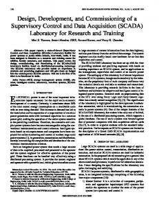
One of the challenging tasks in the wireless charging system is how to align the transmitter and receiver coils. Due to the nature of hydrodynamic interactions between the robotic fish and water, it is hard to make the robotic fish stay still at a specific location to achieve the requirement of maximum power transfer. To address this challenge, we have proposed a charging station for the robotic fish. The charging station consists of (1) docking/holding box which is designed to capture and hold the robotic fish upward to ensure the alignment of the transmitter and receiver coils, (2) linear slider and an actuator for automatically lifting up/down both the holding box and the robotic fish, (3) mechanical frame to attach the entire system to the wall of the swimming tank, and (4) the associated electrical circuitry. The charging station is wirelessly controlled by the main station (PC) through a wireless communication module (XBeePro from Digi). Figure 2.10(a) shows the charging station holding the robotic fish. Figure2.10(b) shows the electrical circuitry of the charging station with the transmitter coil inside the charging and control box. 23
Mechanical Frame
External Power Supply Port
Linear Slider and Actuator
Holding Box
Transmitter and Control Circuitry Box
Robotic Fish
(a)
Wireless Charging Module
Transmitter Coil
Control Circuitry
External Power Supply Jack
(b) Figure 2.10: The charging station: (a) the charging station with the robotic fish, (b) the electrical circuitry of the charging station with the wireless charging module (Model No. (18579694) from Shenzhen Taida Century Technology Co.).
24
2.2.4
Navigation System
The target tracking system consists of an overhead camera (webcam), a touch screen tablet computer, and a wireless communication module. The overhead camera is responsible for capturing a live video of the robotic fish and the swimming tank environment and sending it to the computer. The latter is responsible for three main tasks. First, it performs online processing and analyzes the video to extract the position and orientation data of the robotic fish. Second, it analyzes touches on the screen to identify the target point. Third, it computes and sends actuation commands back to a robotic fish through the wireless communication module. With these commands, the robotic fish will swim to the particular target point. Figure 2.11 shows a schematic representation of the tracking system. Further details of the tracking system can be found in Chapter 5.
Overhead Camera
Main Station
Charging Station
Robotic Fish
Wireless Module Swimming Tank
Wireless Module Touch Screen
Figure 2.11: A schematic representation of the tracking system.
25
2.3
Education and Outreach Activities Using the Robotic Fish
Robotic fish provide not only significant potential research opportunities, but also opportunities for engaging young students and the general public. Robotic fish and other bionic robots have participated in many exhibitions around the world [46, 47]. The first robotic fish prototype has been demonstrated at the 2015 MSU Science Festival (see Figure 2.12). At this event, the MSU Smart Microsystems Lab presented various robotic fish prototypes while the visitors had an opportunity to watch and interact with the robotic fish. The museum robotic fish is scheduled to be deployed at the MSU Museum in Spring 2016, which is expected to have positive impact on local schools, students, and the general public.
26
Figure 2.12: Participation of the first robotic fish prototype in the 2015 MSU Science Festival.
27
Chapter 3 Mathematical Model
3.1
Introduction
Researcher have shown a significant interest in dynamic modeling and control of robotic fish [14, 19, 20, 34, 44, 48, 49]. Many modeling methods and theories have been utilized to capture the fluid-body interactions and the forces and moments on the robotic fish body. Computational fluid dynamics (CFD) modeling has been utilized to capture such interactions [44, 50–52]; however, it is not amenable to control design. Airfoil theory has been used to apply the quasi-steady lift and drag to evaluate the forces on body and fin surfaces of underwater vehicles [20, 53]. J. Wang [44] used Lighthill’s large amplitude elongated-body theory to capture the hydrodynamic forces induced by the interactions between the fluid and a caudal fin-actuated robotic fish. Sanaz et al. [3, 34] modeled a robotic fish actuated by a pair of pectoral fins using blade element theory to calculate the hydrodynamic forces. In this work, we incorporate the rigid body dynamics with the blade element theory [48] and Lighthill’s large amplitude elongated-body theory [49] to model our robotic fish, which is actuated by a caudal fin (tail) and a pair of pectoral fins. For mathematical modeling, we consider the actuation modules and the actuated body. The actuation modules are the tail and pectoral fins, which are the deformable parts of the robotic fish. The body is the undeformable part, and its motion is governed by rigid body dynamics incorporating the added-mass effect. The interaction of the deformable (actuation) 28
modules with the rigid body and the environment (water), and the resulting hydrodynamic forces are evaluated using blade element theory and Lighthill’s large amplitude elongatedbody theory for the pectoral fins and tail fin, respectively. The pectoral fins are designed to perform rowing and spanning motions only. The tail fin is assumed to have no abrupt change on its depth along the length direction, and thus it meets the requirement of an elongatedbody [49]. The proposed modeling approach is amenable to generalization to flexible fins; for ease of discussion, however, we focus on the case of rigid fins actuated at the base point. To provide the background of our work, brief reviews of the rigid body dynamics, blade element theory, and Lighthill’s large amplitude elongated-body theory are presented first.
3.2
Rigid Body Dynamics
Figure 3.1 shows a schematic top view of the robotic fish’s body with two pectoral fins and tail fin. Following the literature [19, 34, 44] on describing the rigid body dynamics, [XY Z] denotes the global (inertial) coordinate system while [x y z] denotes the local (body-fixed) coordinate system with unit vectors [ˆ x, yˆ, zˆ]. The pˆ and tˆ are the perpendicular and parallel unit vectors respectively for each of the pectoral fins. Also, a ˆ and ˆb are the perpendicular and parallel unit vectors respectively for the tail fin. The entire robotic fish body including the pectoral and tail fins is assumed to be neutrally buoyant. Furthermore, it is assumed that the center of mass and the center of geometry of the body coincide at point Cb . The linear and angular velocities of the body at the point Cb are expressed in the local coordinate system. The linear velocity V~C = [u, v, w]T comprises of the x-direction component (u), y-direction b
component (v), and z-direction component (w), which are respectively called surge, sway, ~ = [r, p, q]T consists of three components, which are and heave. Also, the angular velocity Ω
29
Tail fin Pectoral fin Robotic fish body
Figure 3.1: Schematic top view of the robotic fish’s body with a pair of pectoral fins and a tail fin. the roll (r), pitch (p), and yaw (q), respectively. In addition, θ is used to denote the angle of attack of the robotic fish’s body, which is measured from the x-axis to the direction of V~C , ϕ denotes the deflection angle of the pectoral fin with respect to x-axis, β denotes the b
deflection angle of the tail fin with respect to the negative x-axis, and Φ denotes the heading angle of the robotic fish body, formed by the local x-axis with respect to the global X-axis. ~ of the body are respectively The linear momentum and angular momentum P~ and H expressed in the local coordinate system as
~ P~ = Mb · V~C + K T · Ω,
(3.1)
~ = K · V~C + J · Ω, ~ H
(3.2)
b
b
30
where Mb is the mass matrix, J is the inertial matrix, and K is the Coriolis and centripetal matrix. The Kirchhoff’s equations of the motion for a rigid body in an inviscid, irrotational fluid, expressed in the local coordinate system, are given by [44, 54, 55]
˙ ~ + F~ , P~ = P~ × Ω
(3.3)
~˙ = H ~ ×Ω ~ + P~ × V~C + M ~ E, H b
(3.4)
~E = where F~ = [fx , fy , fz ]T denotes the external forces on the body center of mass Cb , M [Mx , My , Mz ]T denotes the external moments about Cb , and (×) denotes the cross product. In this work, we focus on the planar (surface) motion of the robotic fish. Planar motion accompanied with the assumption of neutral buoyancy as well as the body symmetry about the xz-plane, implies that the robotic fish body has only three degrees of freedom, which are the surge (u), sway (v), and yaw (q). Therefore, the heave (w), roll (r), and pitch (p) are all zeros. Furthermore, we assume that the inertial coupling between the surge, sway, and yaw is negligible [19,34,44], which implies that K vanishes as well. With these assumptions, Eq.(3.4) can be reduced to [55]
mx u˙ = my vq + fx ,
(3.5)
my v˙ = −mx uq + fy ,
(3.6)
Iz q˙ = (mx − my )uv + Mz ,
(3.7)
where mx = mb − mxx , my = mb − myy , and Iz = Ib − Izz , mb denotes the mass of the body, Ib denotes the moment of inertia of the body about the z-axis, −mxx and −myy are the added masses in the x- and y-directions, respectively, and −Izz is the added inertial
31
about the z-axis.
3.3
Hydrodynamic Forces and Moments
In the dynamic model (3.5)-(3.7), the external forces fx and fy and the moment Mz are generated due to the interaction between the actuation parts (pectoral and tail fins) with the surrounding fluid. The generated forces and moment are transmitted to the rigid body (robotic fish body). To complete our model, we need to evaluate these hydrodynamic forces and moments. As mentioned in Section 3.1, we use blade element theory and Lighthill’s elongated-body theory to evaluate the hydrodynamic forces generated by the pectoral fins and the tail fin, respectively.
3.3.1
Blade Element Theory
According to blade element theory, the rowing movement of the pectoral fin can be modeled by dividing the fin into a series of small parts (blade elements) and then evaluating the forces on each of these blade elements. After that, the total force of the entire pectoral fin can be determined by integrating these forces along its span length. In the rowing movement of the pectoral fin, there are two significant sub-movements during the fin-beat cycle, power and recovery strokes. In order to gain thrust, real fish tend to change the shape of their pectoral fins in a certain way in each stroke. In the power stroke, the pectoral fin extends to have the maximum interaction area with the surrounding fluid, to produce maximum thrust. On the other hand, the fin is inclined and contracted down to reduce the drag in the recovery stroke. As a result, the fish gains thrust and moves forward. Inspired
32
Joint-base point Base-joint point of pectoral fin
Left pectoral fin
Side view (entire pectoral fin) Robotic fish body Base point of the tail fin
Top view (blade element)
(a)
(b)
Figure 3.2: Configuration of the robotic fish with pectoral and tail fins, a) Schematic representation of the robotic fish with deflated pectoral and tail fins, b) Side and top views of the entire pectoral fin and blade element of the pectoral fin with associated forces and angles respectively. by this biological feature, we have designed the pectoral fins of our robotic fish to change their shapes in both the power and recovery strokes (for further detail see Section 2.1.1.1). However, as mentioned in Section 3.1, we focus on the rigid case of the pectoral fin for the modeling purpose, and thus it is considered as a rectangle-shaped plate with length (span) S and depth (cord) C. Figure 3.2(a) shows a schematic representation of the top view of the robotic fish with deflected pectoral and tail fins, Figure 3.2(b) shows a side view of the entire pectoral fin and a top view of a blade element of the pectoral fin with associated forces and angles. 33
As shown in Figure 3.2(b), the perpendicular force dFp (s, t) and the tangential force dFt (s, t) can be calculated on each small blade element ds at time t as [3, 34, 48] 1 dFp (s, t) = Cp (ψ(s, t))ρCVp 2i (s, t)ds, 2 1 dFt (s, t) = Ct (ψ(s, t))ρCVp 2i (s, t)ds, 2
(3.8) (3.9)
where Vp (s, t) is the velocity of the i-th blade element of the fin, ρ is the density of the surrounding fluid, C is the depth (cord) of the pectoral fin, ψ(s, t) is the angle of attack of the i-th blade element which is given by [48],
tan ψi =
ϕ˙ i r − VC sin ϕi b
VC cos ϕi b
(3.10)
where ϕi and ϕ˙ i are the angular position and velocity of the i-th blade element of the fin respectively and VC is the velocity of the body at the center point Cb . Note that here, for b
simplicity of discussion, we assume that the angle of attack for the body is zero. Cp and Ct are the perpendicular and tangential force coefficients which can be evaluated using the following formula [3, 56]
Cp (ψ(s, t)) = 3.4 sin ψ(s, t), 0.4 cos2 (2ψ(s, t)), for 0 ≤ ψ(s, t) ≤ π/4 Ct (ψ(s, t)) = 0, otherwise
(3.11)
(3.12)
By integrating along the entire pectoral fin, the total hydrodynamic forces for each fin can
34
be determined as Z S Fp (t) =
dFp (s, t)ds,
(3.13)
dFt (s, t)ds,
(3.14)
0 Z S
Ft (t) =
0
The total force FP and FP exerted on the center of mass (Cb ) can be determined by hx hy adding up the forces from both pectoral fins. ~ pL and M ~ pR are the hydrodynamic moments induced by the left and right pectoral fins, M ~ pL can be evaluated respectively, with respect to the center point of the robot body Cb . M by multiplying the total force generated by the left pectoral fin F~pl with the position vector ~rpc which is measured from the point Cb to the base point of the left fin pbl , and it is given by ~ pL = F~pl × ~rpc M
(3.15)
~ pR can be evaluated in the same way. The total hydrodynamic moment The moment M induced by both left and right pectoral fins is given by
~ pT = M ~ pL + M ~ pR M
3.3.2
(3.16)
Lighthill’s Large Amplitude Elongated-body Theory
An elongated-body in Lighthill’s theory [49] could mean a live fish, robotic fish, or a flapping tail fin [44]. In our work, we apply the theory to the flapping tail fin. Following our assumption of planar motion of the robotic fish, the movement of the tail fin will be in the XY -plane. As shown in Figure 3.2(a) (in the deflected tail part) and following the elongated-
35
body theory, a reference frame is considered such that the water far away from the body is at rest. The center line of the elongated-body is parameterized by l, and it is assumed to remain inextensible. The tail base point is represented with l = 0, while the posterior end of the tail is l = L, where L denotes the total length of the elongated-body (tail fin). The trajectory of any point l along the tail at time t is given by (X(l, t), Y (l, t)), where 0 ≤ l ≤ L. The time-dependence of the coordinates could be caused by oscillation/undulation of the tail or as a result of rotational/translational motion of the body [44]. For the hydrodynamic force evaluation, the fin is set in a coordinate system such that an imaginary vertical plane Γ, perpendicular to the tail fin at the posterior end separates between the wake and the tail. Therefore, the tail is contained in a half plane < as shown in Figure 3.2(a). For this situation, there are three components of force in play: the convection of momentum out of < across Γ, the pressure force acting on Γ, and the forces acting on the tail fin which are the reactive forces [49]. These hydrodynamic forces act as a concentrated force at the tail tip (l = L) and a reactive force along the tail (l < L). The concentrated force can be evaluated as
� 1 FLx � 2 ˆ l=L F~L = = − mVT nˆb + mVT n VT t a 2 FLy
(3.17)
and the density of the reactive hydrodynamic force at any point l due to the effect of the added mass along the tail (l < L) can be evaluated as
d Fx (l) f~(l) = ˆ) = −m (VT n a dt Fy (l)
(3.18)
Here VT n and VT t are the normal and tangential components of the tail fin’s velocity, m is 36
the virtual mass per unit length, which can be calculated as 14 πρd2 , where d is the crosssection depth of the fish in Z-direction at each point l (thus function of l), ρ is the density of water, and a ˆ and ˆb are respectively the normal and tangential unit vectors on the tail fin, which can be given by
∂Y a ˆ= − ∂l h
∂X iT , ∂l
iT h ˆb = ∂X ∂Y . ∂l ∂l
(3.19)
The normal VT n and tangential VT t components of the tail fin’s velocity at each point l are given by
∂X ∂Y ∂Y ∂X − , ∂t ∂l ∂t ∂l ∂X ∂X ∂Y ∂Y VT t = + . ∂t ∂l ∂t ∂l VT n =
(3.20) (3.21)
In order to evaluate the hydrodynamic force generated by the tail fin, the velocity of each point of the tail has to be determined over time. Incorporating the rigid body dynamics effect, the velocity at each point along the tail can be evaluated as [44]
V~l = V~C − qcˆ y + (β˙ + q)lˆ a b
(3.22)
where V~C is the linear velocity of the robot body (surge and sway), q is the angular velocity b
of the body (yaw), c denotes the distance from the center of mass of the robot body Cb to the base of the tail fin (l = 0), and β˙ is the angular velocity of the tail fin.
37
Using equations (3.17) - (3.22), we can evaluate the concentrated force at the tail tip as
1 2 ˆ ˆ F~L = − mVLT n b + mVLT n VLT t a 2
(3.23)
The force F~L can be expressed as F~L = FL1ˆb+FL2 a ˆ, where FL1 and FL2 are the components of F~L in ˆb and a ˆ directions, respectively. The hydrodynamic reactive force at each point l can be evaluated as
d 2 f~(l) = −m VlT n, dt
(3.24)
which can be integrated along the tail fin to determine the total hydrodynamic force due to the added mass effect on the tail, and it is given by
F~T = T
Z L 0
f~(l) dl = FT ˆb + FT Tt
Tn
a ˆ,
(3.25)
where FT and FT are the components of F~T in the ˆb and a ˆ directions, respectively. Tt Tn T Finally, the total hydrodynamic forces acting on the tail fin in the x- and y-directions can be expressed as
FT
= −(FL1 + FT ) cos β + (FL2 + FT
) sin β,
(3.26)
FT
= −(FL1 + FT ) sin β − (FL2 + FT
) cos β,
(3.27)
hx hy
Tt
Tn
Tt
Tn
The moment induced by the hydrodynamic forces with respect to the center point Cb has one component about the z-axis due to the assumptions of the planar motion in (XY )-plane,
38
and it can be determined as
MTz = ~rL × F~L +
Z L 0
~rl × f~(l) dl
(3.28)
where ~rl is the positional vector from the center point Cb to any point l on the tail, which is given by, ~rl = −(c + l cos β)ˆ x − (l cos β)ˆ y.
3.3.3
Drag and Lift on the Robot Body
For a rigid body moving in fluid, the latter exerts some forces on the rigid body. These forces are the drag and lift forces with the associated moments, and they are given by [19, 20, 44, 53]
1 Fd = Cd ρSA |VC |2 , b 2 1 Fl = Cl ρSA θ|VC |2 , b 2 Md = −Kd q 2 (q),
(3.29) (3.30) (3.31)
where Cd and Cl are the coefficients of the drag and lift forces, respectively, Kd is the drag moment coefficient, SA denotes the wet surface area of the robotic fish body, and θ is the angle of attack of the robotic fish body. Finally, the total hydrodynamic forces and moments acting on the robotic fish body (fx , fy , and Mz ) in Eq.(3.7) can be calculated by adding the components induced by the pectoral fins, tail fin, and the drag and lift forces and moment exerted by the surrounding
39
fluid,
fx = FP + FT − Fd cos θ + Fl sin θ, hx hx
(3.32)
− Fd sin θ − Fl cos θ,
(3.33)
fy = F P
hy
+ FT
hy
Mz = MpT + MTz + Md ,
3.4
(3.34)
Experimental Validation of the Dynamic Model
Extensive experiments have been conducted to identify and validate the proposed dynamic model. The robotic fish prototype described in Section 2.1 was used in the experiments. Figure 3.3 shows the robotic fish prototype and the experimental setup with Motion Capture Systems. The robot had a pair of pectoral fins and a tail fin for actuation, which were all driven by waterproof servomotors (HS-5086WP from Hitec). The pectoral fin was chosen here specifically for the model validation purpose as a rigid rectangular with 4.86 cm length (span), 3.2 cm height (chord), and 0.2 cm thickness. In order to gain positive thrust from the rigid-rectangular pectoral fin, the fin-beat frequency is set to be different for the power and recovery strokes. We set the frequency of the power stroke five times higher than the frequency of the recovery stroke. As explained in Section 3.3.1, the hydrodynamic force generated by the pectoral fin depends on its velocity and the latter is a function of frequency, so a higher frequency means a higher hydrodynamic force. Therefore, the generated hydrodynamic force in the power stroke is greater than that generated in the recovery stroke, and thus the net resultant will be a positive forward thrust. The tail fin was designed to meet the elongated-body assumptions; in particular, it had a rectangular shape and thus no abrupt change along its length. It was 3D-printed and was 40
8 cm long, 5 cm deep, and 0.2 cm thick. All the pectoral and tail fins were connected directly to the arms of the servomotors. This type of connection allowed the servomotors to control the angular positions (the deflection angles ϕ and β) of the pectoral and tail fins directly. The servomotors were controlled by an embedded-onboard microcontroller (dsPIC30f6014a from Microchip), which was programmed to rotate the pectoral and tail fins according to
ϕ = ϕ◦ + Ap cos(ωp t + ξp ),
(3.35)
β = β◦ + AT sin(ωT t + ξT ),
(3.36)
respectively. Here (ϕ, ϕ◦ , Ap , ωp , ξp ) and (β, β◦ , AT , ωT , ξT ) represent the deflection angle, bias, amplitude, angular frequency, and the phase of the pectoral and tail fins, respectively. During the experiments the tail fin was used for the forward swimming only while the pectoral fins were used for turning and maneuvering. As in the literature [34, 44], we measured the steady-state forward velocity, turning radius, and turning period versus the actuation frequency to validate our model. The experiments were done in a medium-sized tank (185 cm ×65 cm) as shown in Figure 3.3. The measurements of the forward velocity, turning radius, and turning period were done using the OptiTrack Motion Capture Systems. Each experiment was repeated five times to obtain the average and standard deviation. Before the results are presented and discussed, all the parameters of the robotic fish model should be identified.
41
OptiTrack System Software
Tracking System Cameras
Swimming Area
Tracking Markers
Robotic Fish
Figure 3.3: Experimental setup with the Motion Capture Systems. Table 3.1: Parameter values of the body for simulation.
Component Parameter Body
Value
Body mass (mb ) Wet surface area of the body (SA )
0.04248 m2
Distance from center of the body to the joint (c)
0.098806 m
Moment of inertia of the body
Pectoral fin Tail fin General
0.76 kg
24.73 × 10⁻⁴ kg.m2
−mxx
0.0422 kg
−myy
0.3157 kg
−Izz
4.1662 × 10⁻⁴ kg.m2
Pectoral fin length (S)
0.0486 m
Pectoral fin width (C)
0.032 m
Tail length (L)
0.08 m
Tail width (d)
0.05 m 1000 kg/m2
Water density (ρ)
42
3.4.1
Parameter Identification
Table 3.1 provides the parameters of the robotic fish body. These parameters were either measured directly or calculated. First, we calculate the effect of added inertia and mass by considering the robot body as a prolate spheroid which has a profile given by [19, 44, 54] x2 y 2 + z 2 + =1 a2 b2
(3.37)
where a and b are the semi-axes of the prolate spheroid. For our robotic fish body, a and b values are set to 9.8806 cm and 3.305 cm, respectively, to match the geometric parameters of the body. For the prolate spheroid, the added mass and inertia effects can be determined by
mxx = −k1 ma ,
(3.38)
myy = −k2 ma ,
(3.39)
Izz = −k3 Iaz ,
(3.40)
where ma denotes the displaced water’s mass, which is determined by ma = 43 ρπab2 , Iaz denotes the moment of inertia of the spheroidal water mass Iaz = 51 ma (a2 + b2 ), and k1 , k2 and k3 are the Lamb’s k-factors which are positive and dependent on the geome-
43
try of the submerged body, and they can be evaluated as [19, 44]
µ , 2−µ η k2 = , 2−η
(3.41)
k1 =
k3 =
(3.42)
e4 (η − µ) , (2 − e2 )[2e2 − (2 − e2 )(η − µ)]
(3.43)
where � 2(1 − e2 ) � 1 (1 + e) ln −e , 3 2 (1 − e) e 2 1−e (1 + e) 1 ln , η= 2− 3 (1 − e) e 2e µ=
(3.44) (3.45)
2 and e2 = 1 − b 2 is the ellipsoid’s eccentricity. a
1 m (2c)2 , The moment of inertia of the robot body about z-axis is determined by Ib = 12 b
where c is the distance from the center point Cb to the joint point J. Finally, the drag, lift, and drag moment coefficients, Cd , Cl , and Kd , can be obtained in several ways such as CFD simulation, water tunnel tests, and empirical fitting. In our work, the coefficients Cd = 0.285, Cl = 3.1, and Kd = 18 × 10−3 were obtained empirically by tuning these parameters, so that the simulation results match the experimental ones. The tuning process was achieved under a particular setup pattern for the pectoral and tail fins, with (ϕ◦ = 0, Ap = 45◦ , ωp = π rad/s (0.5 Hz for power stroke), ξp = 0) and (β◦ = 0, AT = 20◦ , ωT = π rad/s (0.5 Hz), ξT = 0), respectively. Then, the resulting coefficients were used in independent model validation for the other patterns.
44
3.4.2
Simulation and Experimental Results
Figures 3.4 - 3.6 show the results of the simulation compared with those obtained from experiments. As mentioned in Section 3.4, we measured the forward velocity, and turning radius and period to validate the dynamic model. The bias and amplitude were held constant (ϕ◦ = 0, Ap = 45◦ ) and (β◦ = 0, AT = 20◦ ) for the pectoral and tail fins, respectively, while we varied the frequency. 16 Experimental Simulation
14
Velocity in cm/s
12 10 8 6 4 2 0 0
0.5
1
1.5 2 Frequency (Hz)
2.5
3
3.5
Figure 3.4: Simulation and experimental results of the forward velocity.
From the results in Figure 3.4, we can see that the forward velocity increases as the frequency increases. It is obvious that the model closely captures the dynamic of the system; however, at the higher frequencies the experimental results show saturation, which was due to the mechanical limitation of the actuators (servomotors). On the other hand, from Figures 3.5 and 3.6, the turning period decreases while the turning radius remains constant as the frequency increases. Also, from the results in Figure 3.5, we can see the effect of the actuators’
45
120 Experimental Simulation
Turning Time in sec
100
80
60
40
20
0 0
0.5
1
1.5 2 Frequency (Hz)
2.5
3
3.5
Figure 3.5: Simulation and experimental results of the turning period.
45 Experimental Simulation
40
Turning Raduis in cm
35 30 25 20 15 10 5 0 0
0.5
1
1.5 2 Frequency (Hz)
2.5
3
3.5
Figure 3.6: Simulation and experimental results of the turning radius.
46
mechanical limitation at higher frequencies. Over all, from the results, we can see that the model can predict closely the behavior of the robotic fish system.
3.5
Comparison of Multi-Segment Versus Rigid Pectoral Fins
In the mathematical model of the robotic fish system, only the rigid case of the pectoral fin has been investigated. In order to validate the high hydrodynamic performance of the proposed pectoral fin design, some experiments have been conducted to compare the hydrodynamic performance of the robotic fish using multi-segment pectoral fin and the rigid pectoral fin. The comparison was done in terms of the turning period and radius. Figures 3.7 and 3.8 show the results of the comparison. From the results in Figure 3.7, it is clear that using the multi-segment pectoral fin reduces the turning period, which means improving the maneuverability of the robotic fish. In addition, it results in a tighter turning radius as shown in Figure 3.8, further supporting that the new pectoral fin design has a superior maneuvering performance.
47
120 Rigid Multi−segments
110
Turning Time in sec
100 90 80 70 60 50 40 30 20 10 0
0.5
1
1.5 2 Frequency (Hz)
2.5
3
3.5
Figure 3.7: Experimental results on the comparison of the turning period of the robotic fish when using multi-segment pectoral fins and rigid pectoral fins, respectively.
30
Turning Raduis in cm
Rigid Multi−segments
25
20
15 0
0.5
1
1.5 2 Frequency (Hz)
2.5
3
3.5
Figure 3.8: Experimental results on the comparison of the turning radius of the robotic fish when using multi-segment pectoral fins and rigid pectoral fins, respectively.
48
Chapter 4 A Wireless Charging System for Robotic Fish
4.1
Introduction
Autonomous robots are powered by on-board power supplies. Batteries have being widely used as the on-board power sources. Because of the limited capacity of the batteries, they need to be recharged routinely. The conventional method of recharging is wired charging, which needs human intervention. In particular, wired charging requires the robot to be taken off the field of work. Researchers have explored many techniques to overcome this problem. James et al. [57] designed an on-station recharging system using solar cells. This system was designed to improve the performance of autonomous underwater vehicles (AUV’s) for longduration tasks. Autonomous docking is an another technique for recharging. This technique was developed for commercial robots such as irobots’ Roomba, which is a vacuuming robot [58]. In autonomous docking the robot goes to a recharging station and makes direct physical contact with the charger [59]. Using the same principle, but in a different way, Brike [60] developed an autonomous recharging system for mobile robots. In this system the charging station consists of two metal plates connected to a regulated power supply. The first plate is on the floor and the second plate is horizontally above the first one. The robot has two points of contact above and underneath it. These points of contact touch the two charging 49
station’s plates to start the recharging process. All of the techniques mentioned above are either designed for outdoor applications or they require a direct physical contact with the chargers. Both situations are not applicable for a small robotic fish, especially for indoor applications. To overcome this problem, we have designed and developed a wireless charging system. The charging scheme exploits wireless power transfer (WPT), which is based on electromagnetic induction and magnetic resonance [36, 37, 61–66]. When an alternating current (AC) flows into a coil (transmitter) with a number of turns (N ), an alternating magnetic field proportional to the AC current and the number of turns will be generated. If the generated magnetic field intersects another coil (receiver), an alternating current will be induced and flow into the receiver coil. The induced AC current can be used directly or converted into a direct current (DC) by a rectifying circuit. The DC current can be used to recharge the battery of an autonomous robot. Figure 4.1 shows a schematic representation of the wireless charging system. During this process, the power will be transferred wirelessly between the transmitter and receiver coils. By the electromagnetic principle, the two coils must be close to each other with proper alignment to achieve maximum power transfer and maximum efficiency. If the coils are separated for some distance, the received power will drop significantly [63]. A well-known example of wireless inductive charging is the charging system for electric toothbrushes. To achieve maximum power transfer and high efficiency in the mid-range distances, magnetic resonance coupling and strong resonance coupling have been utilized [36,37,61,63–65]. The resonance happens between an inductor and a capacitor in the LC-loop circuit at a specific frequency, called the resonance frequency (ω) given by
ω=√ 50
1 LC
(4.1)
Figure 4.1: Schematic representation of the wireless charging system. where L is the inductance of the coil and C is the capacitance.
4.2
Mathematical Model
The magnetic resonant system represented by the equivalent circuit shown in Figure 4.2 is adopted for mathematical modeling and analysis based on electrical circuit theory. Here M is the mutual inductance between the transmitter and receiver coils, K is the coupling coefficient, and d is the distance of separation. L1 and L2 are the self-inductances of the transmitter and receiver coils, respectively, and R1 , R2 , C1 and C2 are the internal resistances of the coils and the capacitances of the transmitter and receiver circuits respectively. RL denotes the load resistance. The system is supposed to work at the resonance frequency ω which is given in Eq.(4.1). For the convenience of analysis, some assumptions and manipulations are considered as follows [4]: • The currents i1 (t) and i2 (t) are integrated for the transmitter and receiver coils as a single coil current. • The voltage source v(t) and the transmitter capacitor C1 are grouped together to serve 51
Figure 4.2: Magnetic resonant system equivalent circuit, adapted from [4]. as a unified voltage source vin (t), as indicated by the dotted box in Figure 4.2. This operation is valid because the transmitter coil is driven by v(t) itself, while C1 just makes the current i1 (t) bypass the source v(t). • The receiver capacitance C2 and the load resistance RL are combined together to form a complex impedance zL , as indicated by the dotted box in Figure 4.2. • The system is at the steady state, and the unified voltage source with the integrated coils’ currents are expressed in exponential form, where: v(t) = V ejωt , i1 (t) = I1 ejωt , and i2 (t) = I2 ejωt . • The amplitude of the unified voltage source V is set to be a real number, while the currents’ amplitudes might be complex numbers to indicate the phase shift between the voltage source and the currents. From the considerations above, Kirchhoff’s voltage equations for the transmitter and receiver circuits can be readily written as:
52
jωM R1 + jωL1 I1 V = jωM R2 + jωL2 + zL I2 0
(4.2)
The impedance zL is given by
zL =
2X RL RL Xc2 c − j 2 2 2 RL + Xc RL + Xc2
(4.3)
1 . where Xc = ωC 2
From Eq.(4.2), the currents I1 and I2 can be determined as
I1 =
[(R2 + a) + j(ωL2 − b)]V , [R1 (R2 + a) − ωL1 (ωL2 − b) + (ωM )2 ] + j[R1 (ωL2 − b) + ωL1 (R2 + a)]
(4.4)
I2 =
−jωM V , [R1 (R2 + a) − ωL1 (ωL2 − b) + (ωM )2 ] + j[R1 (ωL2 − b) + ωL1 (R2 + a)]
(4.5)
where a and b are the real and imaginary parts of zL = a + jb, respectively.The input and output powers can then be evaluated as [4]:
1 Pin = V