recycle [41,44]. Considering Apple Computer's Electronic. Recycling Program in United States and Canada [49], the EOL. Power Mac G4 Cubes® are assumed ...
Proceedings of IDETC/CIE 2006 ASME 2006 International Design Engineering Technical Conferences & Computers and Information in Engineering Conference September 10-13, 2006, Philadelphia, Pennsylvania, USA
DETC2006-99475 DESIGN FOR OPTIMAL END-OF-LIFE SCENARIO VIA PRODUCT-EMBEDDED DISASSEMBLY Shingo Takeuchi and Kazuhiro Saitou Department of Mechanical Engineering University of Michigan Ann Arbor, MI, 48109-2125 E-mail:{stakeuch, kazu}@umich.edu
ABSTRACT This paper presents a computational method for designing products with a built-in disassembly means that can be triggered by the removal of one or a few fasteners at the end of the product lives. Given component geometries, the method simultaneously determines the spatial configuration of components, locators and fasteners, and the end-of-life (EOL) treatments of components and subassemblies, such that the product can be disassembled for the maxim profit and minimum environmental impact through recycling and reuse via domino-like “self-disassembly” process. As an extension of our previous work, the present method incorporates EOL treatments of disassembled components and subassemblies as additional decision variables, and the Life Cycle Assessments (LCA) focusing on EOL treatments as a means to evaluate environmental impacts. A multi-objective genetic algorithm is utilized to search for Pareto optimal designs in terms of 1) satisfaction of the distance specification among components, 2) efficient use of locators on components, 3) profit of EOL scenario, and 4) environmental impact of EOL scenario. The method is applied to a simplified model of Power Mac G4 cube® for demonstration. INTRODUCTION Economic feasibility of an end-of-life (EOL) scenario of a product is determined by the interaction among disassembly cost, revenue from the EOL treatments of the disassembled components, and the regulatory requirements on products, components and materials. While meeting regulatory requirements is obligatory regardless of economic feasibility, EOL decision making is often governed by economical considerations [1]. Even if a component has high recycling/reuse value or high environmental impact, for
instance, it may not be economically justifiable to retrieve it if doing so requires excessive disassembly cost. Since the cost of manual disassembly depends largely on the number of fasteners to be removed and of components to be reached, grabbed, and handled during disassembly, it is highly desirable to locate such high-valued or high-impact components within a product enclosure, such that they can be retrieved by removing less number of fasteners and components. reuse
landfill
A A B
C
reuse A B
B
C
B
C
(a) reuse
recycle
B
C C
C (b)
recycle
Figure 1. (a) Conventional assembly (b) assembly with embedded disassembly.
As a solution to this problem, we have previously introduced a concept of product-embedded disassembly [2, 3], where components are spatially arranged within a product enclosure such that they can be reached and removed in an optimal sequence. In order to minimize the number of fasteners, the relative motions of components are constrained, wherever possible, by locators (eg., catches, lugs, tracks and bosses) integrated to components.
1
Copyright © 2006 by ASME
Figure 1 illustrates the concept of product-embedded disassembly as compare to the conventional disassembly. In the conventional assembly (Figure 1 (a)), components A, B and C are fixed with three fasteners. With high labor cost for removing fasteners (as often the case in developed countries), only A may be economically disassembled and reused, with the remainder sent to landfill. This end-of-life (EOL) scenario (i.e., disassemble and reuse A, and landfill the remainder) is obviously not ideal both from economical and environmental viewpoints. In the assembly with embedded disassembly (Figure 1 (b)), on the other hand, the motions of B and C are constrained by the locators on components. As such, the removal of the fastener to A (called a trigger fastener) activates the domino-like self-disassembly pathway AÆBÆC. Since no additional fasteners need to be removed, B and C can also be disassembled, allowing the recycle/reuse of all components and the case. This EOL scenario (i.e., disassemble all components, reuse A and B, and recyle C and the case) is economically and environmentally far better than the one for the conventional assembly.
(a)
(b)
Figure 2. Example products suited for product-embedded disassembly, (a) desktop computer (b) DVD player.
The concept of product-embedded disassembly can be applied to a wide variety of products, since it requires no special tools, materials, or actuators to implement. It is particularly well suited for electrical products assembled of functionally modularized components, whose spatial configurations within the enclosure have some flexibility. Figure 2 shows examples of such products. A desktop computer in Figure 2 (a) is assembled of functionally distinct components such as a motherboard, a hard drive, and a power unit, arranged to fit within a tight enclosure. The components are, however, not completely packed due to the need of the air passage for cooling and the accessibility for upgrade and repair. Thanks to this extra space and electrical connections among components, the spatial configurations of the components have a certain degree of flexibility. A DVD player in Figure 2 (b) even shows roomier component arrangements, due to the consumers’ tendency to prefer large sizes in home theater appliances. Since designing products with single “disassembly button” may cause safety concerns, the method will, in practice, be best utilized as an inspiration to the designer during the early stage
configuration design and critical components can be independently fastened with a secure, conventional means. The concept, however, may be unsuitable to the products that allow very little freedom in component arrangements. Examples include mobile IT products such as cell phones, laptop computers, MP3 players, due to their extremely tight packaging requirements and mostly layer-by-layer assembly. This paper presents an extension of our previous work [2, 3], where the problem was posed as optimization of the arrangements of components, locators and fasteners, to merely maximize the profit of disassembly. In [2, 3], the profits of components via EOL treatments are considered as constant and given as inputs to the problem. Although one should always assume the most profitable EOL treatments (or non-treatments) for maximizing overall profit, it is well known that this would not be always optimal for minimizing environmental impacts. In order to examine a trade-off between the overall profit and the environmental impacts of EOL scenarios, the present work newly incorporates the EOL treatments of disassembled components and subassemblies as additional decision variables, and the Life Cycle Assessments (LCA) focusing on EOL treatments as a means to evaluate environmental impacts. A multi-objective genetic algorithm [4, 5] is utilized to search for Pareto optimal designs in terms of 1) satisfaction of the distance specification among components, 2) efficient use of locators on components, 3) profit of the EOL scenario of the product, and 4) environmental impact of EOL scenario obtained by LCA. The method is applied to a simplified model of Power Mac G4 cube® for demonstration. RELATED WORK Design for Disassembly Design for disassembly (DFD) is a class of design method and guidelines to enhance the ease of disassembly for product maintenance and/or EOL treatments such as recycling and reuse [6-8]. As in the case of design for assembly (DFA), the estimation of disassembly time has been a central focus of the research on DFD [9, 10], since it is a major driver of disassembly cost and consequently, the economic feasibility of the EOL scenarios that require disassembly [11]. Recently, Desai et al. [12] developed a scoring system, where factors associated with disassembly time such as disassembly force, the requirement of tools and the accessibility of fasteners are considered. Sodhi et al. [13] focused on the impact of unfastening actions on disassembly cost and constructed Ueffort model that helps designers to select fasteners for easy disassembly. While these works help identify problems in existing assemblies and suggest local redesigns to improve the ease of disassembly, they do not address the improvement of an entire disassembly processes by the global changes in the component, locator, and fastener configurations, as addressed in this paper.
2
Copyright © 2006 by ASME
Disassembly Sequence Planning
Disassembly sequence planning (DSP) aims at generating feasible disassembly sequences for a given assembly, where the feasibility is checked by the existence of collision-free motions to disassemble components. Since the problem is NP-complete, the past researches have focused on efficient heuristic algorithms to approximately solve the problem. Based on assembly sequence planning [14-18], algorithms for disassembly sequence generation have been developed [19-21]. More recent works are geared towards DSP with special attention to reuse, recycling, remanufacturing, and maintenance [22-26]. Chung et al. [27] modified the wave propagation method [23] to solve DSP, by considering both disassemblability of components and accessibility of fasteners. Kuo [28] found the most profitable EOL scenario of electromechanical products by examining all feasible disassembly sequences. Seo et al. [29] considered both economical and environmental costs to obtain the optimal disassembly sequence. These works, however, only address the generation and optimization of the disassembly sequences for products with a pre-specified component layout. Since the accessibility of a component heavily depends on the spatial configuration of its surrounding components, this would seriously limit the opportunity for optimizing an entire assembly. In addition, these works do not address the design of locator and fastener configurations, which also have a profound impact on the feasibility and quality of a disassembly sequence.
of various products [37,38] including computers [39-41]. Since the optimal EOL scenario should be economically feasible as well as environmentally sound, LCA is often integrated with cost analysis. Goggin et al. [42] constructed a model for determining the recovery of a product, components and materials, where EOL scenarios are evaluated from economical and environmental perspectives. Kuo et al. [43] integrated LCA into Quality Function Development (QFD) to achieve the best balance between customer satisfaction and environmental impact. In our previous work [44], we compared the optimal EOL scenarios of a coffee maker in Aachen, Germany and in Ann Arbor, MI, and concluded the optimal EOL scenario varied greatly depending on the local recycling/reuse infrastructures and regulatory requirements. These works, however, merely address the evaluation and optimization of the environmental impact of a given product, and do not address the design of component, locator, and fastener configuration as addressed in this paper. METHOD The method can be summarized as the following optimization problem: •
•
Configuration Design Problem
While rarely discussed in the context of disassembly, the design of spatial configuration of given shapes has been an active research area by itself. Among the most popular flavors is bin packing problem (BPP), where the total volume (or area for 2D problem) occupied by the given shapes is minimized. Since this problem is also NP-complete, heuristic methods are commonly used. Corcoran and Wainwright [30] solved a 3D BPP with genetic algorithm (GA). Kolli et al. [31] used multiresolution quad trees and simulated annealing to solve a 2D BPP using. Jain and Gea [32] solved a packing problem of 2D shapes represented by pixels. Fadel et al. [33] used virtual rubber band to solve a 3D BBP. As a variant of BPP, the layout design problem has been also widely studied. Fujita et al. [34] solved a 2D plant layout design problem by simulated annealing and the generalized reduced gradient (GRG) method. Grangeon et al. [35] addressed a 3D layout design of a steel sheet manufacturing workshop. Grignon and Fadel [36] presented a 3D layout design problem considering static and dynamic balance, maintainability and volume. These works, however, do not address the integration with DSP as addressed in this paper. Life Cycle Assessment
• • •
Given: geometries, weights, materials, and recycle and reuse values of each component, contact and distance specifications among components, locator library, and possible EOL treatments and associated scenarios. Find: spatial configuration of components and locators, EOL treatments of disassembled components and subassemblies. Subject to: no overlap among components, no unfixed components prior to disassembly, satisfaction of contact specification, assembleability of components. Minimizing: violation of distance specification, redundant use of locators, and environmental impact of EOL scenario. Maximizing: profit of EOL scenario.
Since the optimization problem has four objectives, a multi-objective genetic algorithm (MOGA) [4, 5] is utilized to obtain Pareto optimal solutions. Inputs
There are four (4) categories of inputs for the problem as listed below: •
•
Life cycle assessment (LCA) has been widely used as a tool to estimate the environmental impacts of an EOL scenario
3
Component information: This includes the geometries, weights, materials and reuse values of components. Due to the efficiency in checking contacts [45] and the simplicity in modifying geometries, the component geometry is represented by voxels. Contact and distance specifications: The contact specification specifies the required adjacencies among the component, such as CPU and a heat sink in a computer. The distance specification specifies the relative importance
Copyright © 2006 by ASME
•
•
(weight) of minimizing the distances between each pair of the components, eg., for wire connections. Figure 3 shows an example. Locator library: This is a set of locator features that can be added on each component to constrain its relative motion. Types of locators in the library depend on the application domain. Figure 4 shows schematics of locators commonly found on sheet metal or injection-molded components in computer assemblies [46]. Note screws are regarded as a special type of locators, and slot can only be used with two circuit boards. Possible EOL treatments and scenarios: An EOL scenario is a sequence of events, such as disassembly, cleaning, and refurbishing, before a component receives an EOL treatment such as recycle and reuse. The EOL treatments available to each component and the associated scenarios leading to each treatment must be given as input. Figure 5 shows an example of EOL treatments (reuse, recycle, or landfill) and the associated EOL scenarios represented as a flow chart.
ti ∈{0, ±c, ±2c, ±3c, ...}3 ri ∈{-90o, 0 o, 90 o, 180 o}3 di ∈{0, ±c, ±2c, ±3c, ...}f
(3) (4) (5)
where n is the number of components in the assembly, ti and ri are the vectors of the translational and rotational motions of component i with respect to the global reference frame, and di is a vector of the offset values of the f faces of component i in their normal directions, and c is the length of the sides of a voxel. Note that di is considered only for the components whose dimensions can be adjusted to allow the addition of certain locator features. For example, the components designed and manufactured in-house can have some flexibility in their dimensions, whereas off-the-shelf components cannot. Assembly Subassembly Landfill?
Yes
Landfill
No Single component? No Disassemble
Yes
Reuse? No Shred
Yes
Refurbish Reuse
Recycle
Figure 5. Flow chart of example EOL scenarios. Figure 3. Example of contact specification (thick line) and distance specification (thin lines). Labels on thin lines indicate relative importance of minimizing distances.
The second design variable, locator vector, represents the spatial configuration of the locators on each component: y = (y0, y1, …, ym-1) yi = (CDi, pi); i = 0, …, m-1
(a)
(b)
(c)
(d)
(e)
(f
Figure 4. Graphical representation of typical) locators for sheet metal or injection-molded components [46]: (a) catch, (b) lug, (c) track, (d) boss, (e) screw, (f) slot. Design variables
There are three (3) design variables for the problem. The first design variable, configuration vector, represents the spatial configuration and dimensional change of each component: x = (x0, x1, …., xn-1) xi = (ti, ri, di,); i = 0, 1, … n-1
(1) (2)
(6) (7)
where m = n (n-1)/2 is the number of pairs of components in the assembly, and CDi ⊆ {-x, +x, -y, +y, -z, +z} is a set of directions in which the motion of component c0 in the i-th pair (c0, c1) is to be constrained, and pi is a sequence of locators indicating their priority during the construction of the locator configuration. The choice of locator for the i-th component pair is indirectly represented by CDi and pi, since the direct representation of locator id in the library would result in a large number of infeasible choices. The construction of locator configurations from a given yi is not trivial since 1) multiple locator types can constrain the motion of c0 as specified by CDi, and 2) among such locator types, geometrically feasible locators depend on the relative locations of components c0 and c1. Figure 6 shows an example. In order to constrain the motion of c0 in +z direction, a catch can be added to c1 if c0 is “below” c1 as shown in Figure 6 (a). However, a catch cannot be used if c0 is “above” c1 as shown in Figures 6 (b) and (c), in which case boss (Figure 6 (b)) or track (Figure 6 (c)) needs to be used.
4
Copyright © 2006 by ASME
Thus, the locator configuration of a component is dynamically constructed by testing locator types in the sequence of pi. More details of the locator vector are found in [2]. +
+z
c1
+
c0
c0 c1
c0 (a)
c1 (b)
(c)
Figure 6. Construction of locator configuration.
f 2 ( x , y ) = ∑ mc i
where mci is the manufacturing difficulty of the i-th locator in the assembly, which represents the increased difficulty in manufacturing components due to the addition of the i-th locator. The third objective function (to be maximized) is the profit of the EOL scenario of the assembly specified by x and y, given as: n −1
f 3 ( x , y, z ) = ∑ p i ( z i ) − c * ( x, y, z )
The third design variable, EOL vector, represents the EOL treatments of components: z = (z0, z1, …., zn-1) zi ∈ Ei
(11)
i
(8) (9)
where Ei is a set of feasible EOL treatments of component i. In the following case study, Ei = {recycle, reuse, landfill} for all components.
(12)
i =0
In Equation 12, pi(zi) is the profit of the i-th component from EOL treatment zi, calculated by the LCA model described in the next section. Also in Equation 12, c*(x, y, z) is the minimum disassembly cost the assembly under the EOL scenario required by z: c * ( x , y, z ) = min c( s ) s∈S xyz
Constraints
(13)
There are four (4) constraints for the problem: 1. 2. 3. 4.
No overlap among components. Satisfaction of contact specification. No unfixed components prior to disassembly. Assembleability of components.
Since the constraints are all geometric in nature, the voxel representation of component geometry facilitates their efficient evaluation. Constraints 1-3 are checked solely based on the information in x, since the locator configurations constructed from y generate no overlaps. For constrain 3, immobility of all possible subassemblies is examined. Constraint 4 is necessary to ensure all components, weather or not to be disassembled, can be assembled when the product is first put together. It requires the information both x and y. Since checking this constraint requires simulation of assembly motions (assumed as the reverse of disassembly motions), it is done as a part of the evaluation of disassembly cost needed for one of the objective functions.
where Sxyz is the set of the partial and total disassembly sequences of the assembly specified by x and y, for retrieving the components with zi = reuse or recycle and the components with regulatory requirement, and c(s) is the cost of disassembly sequence s. Since an assembly specified by x and y can be disassembled in multiple sequences, Equation 13 computes the minimum cost over Sxyz, which contains all disassembly sequences feasible to x, y, and z, and their subsequences. Set Sxyz is represented as AND/OR graph [14], computed based on the 2-disassemblability criterion [19, 45] (component can be removed by up to two successive motions) as follows: 1. 2. 3.
4.
Objective functions
There are four (4) objective functions for the problem. The first objective function (to be minimized) is for the satisfaction of the distance specification, given as: f 1 ( x , y ) = ∑ wi d i
(10)
i
where wi is the weight of the importance of distance di between two designated voxels. The second objective function (to be minimized) is for the efficient use of locators, given as:
5.
Push the assembly to stack Q and the AND/OR graph. Pop a subassembly sa from Q. If sa does not contains component with zi = reuse or recycle and components with regulatory retrieval requirements, go to step 5. For each subassembly sb ⊂ sa that does not contain any fixed components, check the 2-disassemblability of sb from sa. If sb is 2-disassemblable, add sb and sc = sa\sb to the AND/OR graph. If sb and/or sc are composed of multiple components, push them to Q. If Q = Ø, return. Otherwise go to step 2.
For efficiency, only translational motions are considered during the 2-disassembleabilty check in step 4. Assuming manual handling, insertion and fastening as timed in [47], c(s) is estimated based on the motions of the components and the numbers and accessibilities of the removed screws at each disassembly step. The accessibility of a removed screw is given as [2]:
5
Copyright © 2006 by ASME
as = 1.0 + ωa / (aa + 0.01)
(14)
where ωa is weight and aa is the area of the mounting face of the screw, accessible from outside of the product in its normal direction. The forth objective function (to be minimized) is the environmental impact of the EOL scenario: f 4 ( z ) = ∑ ei ( zi )
high revenue and high energy recovery. The availability of the reuse option for a component, however, is infrastructure dependent, and even if available, the revenue from reuse can greatly fluctuate in the market and hence difficult to estimate a priori. Revenue from recycle rirecycle and energy consumption of recycle eirecycle are also calculated based on the material composition of a component:
(15)
rirecycle =
i
∑ mr
recycle ⋅ mij j
(19)
j
where ei(zi) is the environmental impact of i-th component according to the EOL scenario for treatment zi. The value of ei(zi) is estimated by the LCA model described in the next section. LCA model
The LCA model adopted in the following case study focuses on EOL treatments and assumes the EOL scenarios in Figure 5 for all components (reuse for some components only), and energy consumption as the indicator for environmental impact [44]. Accordingly, profit pi(zi) in Equation 12 is defined as: ⎧ri reuse − c itrans − c irefurb ⎪ p i ( z i ) = ⎨ri recycle − c itrans − c ishred ⎪− c trans − c landfill i ⎩ i
if z i = reuse if z i = recycle
if z i = reuse
(17)
where eireuse, eitrans, eirecycle, eirefurb, eishred and eilandfill are the energy consumptions of reuse, transportation, recycle, refurbishment, shredding, and landfill, respectively. Revenue from reuse rireuse is the current market value of component i, if such markets exist. Energy consumption of reuse eireuse is the negative of the energy recovered from reusing component i:
eireuse = −
∑ me
intens j
⋅ mij
recover j
⋅ mij
(20)
j
where mrjrecycle and mejrecover are the material value and recovered energy of material j, respectively. Since few data is available for the refurbishment of components, the cost for refurbishment is simply assumed as:
cirefurb= 0.5·rireuse
(21)
Based on the data on desktop computers [40], energy consumption for refurbishment eirefurb is estimated as: (22)
(16)
if z i = landfill
if z i = recycle if z i = landfill
∑ me
eirefurb = 1.106 · mi
where rireuse and rirecycle are the revenues from reuse and recycle, respectively, and citrans, cirefurb, cishred and cilandfill are the cost for transportation, refurbishment, shredding, and landfill, respectively. Similarly, energy consumption ei(zi) in Equation 15 is defined as: ⎧eireuse + eitrans + eirefurb ⎪ ei ( z i ) = ⎨eirecycle + eitrans + e ishred ⎪e landfill + e trans i ⎩ i
eirecycle = −
(18)
j
where mejintens is the energy intensity of material j and mij is the weight of material j in component i. Reuse, if available, is usually the best EOL treatment for a component because of its
where mi is the weight of the i-th component. Cost and energy consumption of transportation citrans and trans are estimated as [44]: ei
citrans = Δcitrans · Di · mi eitrans = Δeitrans · Di · mi
(22) (23)
where Δcitrans =2.07e-4 [$/kg·km], Δeitrans =1.17e-3 [MJ/kg·km], and Di is the travel distance. Similarly, costs and energy consumptions for shredding and landfill cishred , cilandfill, eishred and eilandfill are calculated as [44]:
cishred = Δcishred · mi eishred = Δeishred · mi cilandfill = Δcilandfill · mi eilandfill = Δeilandfill · mi
(24) (25) (26) (27)
where Δcishred = 0.12 [$/kg·km], Δeishred = 1.0 [MJ/kg·km], Δcilandfill = 0.02 [$/kg·km] and Δeilandfill = 20000 [MJ/kg·km]. Optimization algorithm Since the problem is essentially a “double loop” of two NP-complete problems (disassembly sequence planning within a 3D layout problem), it should be solved by a heuristic algorithm. Since design variables x, y, z are discrete (x is a discrete variable since geometry is represented as voxels) and there are four objectives, a multi-objective genetic algorithm [4,5] is utilized to obtain Pareto optimal design alternatives. A
6
Copyright © 2006 by ASME
multi-objective genetic algorithm is an extension of the conventional (single-objective) genetic algorithms that do not require multiple objectives to be aggregated to one value, for example, as a weighted sum. Instead of static aggregates such as a weighted sum, it dynamically determine an aggregate of multiple objective values of a solution based on its relative quality in the current population, typically as the degree to which the solution dominates others in the current population. A chromosome, a representation of design variables in genetic algorithms, is a simple list of the 3 design variables:
c = (x, y, z)
(28)
Since the information in x, y, and z are linked to the geometry of a candidate design, the conventional one point or multiple point crossover for linear chromosomes are ineffective in preserving high-quality building blocks. Accordingly, a geometry-based crossover operation is used as in [2]. CASE STUDY
composition data in [48] is utilized. Table 3 shows energy intensity mejintens, recovered energy mejrecove, and material values mrjrecycle [41,44]. Considering Apple Computer’s Electronic Recycling Program in United States and Canada [49], the EOL Power Mac G4 Cubes® are assumed to be transported to one of two facilities in United States (Worcester, MA and Gilroy, CA) for reuse, recycle, and landfill. The average distance between the collection point and the facility is estimated as Di = 1000 km for all components. It is assumed that 40 ton tracks are used for transportation. Based on this assumption, Table 4 shows the revenues, costs and energy consumptions of components A-J calculated using Equations 18-27. Revenue from reuse rireuse reflects current values in the PC reuse markets in the United States [50, 51]. Note that reuse option is not available to components A (frame) and B (heat sink). Table 1. Relative manufacturing difficulty of the locators in the locator library in Figure 4
Locator Mfg. difficulty
Lug 20
Track Catch 30 10
Problem The method is applied to a model of Power Mac G4 Cube® manufactured by Apple Computer, Inc. (Figure 7). Ten (10) major components are chosen based on the expected contribution to profit and environmental impact. Figure 8 (a) shows the ten components and their primary liaisons, and Figure 8 (b) shows the voxel representation of their simplified geometry and the contact (thick lines) and distance (thin lines with weights) specifications. The contacts between component B (heat sink) and C (CPU), and C (circuit board) and G (memory) are required due to their importance to the product function. Component A (case) is considered as fixed in the global reference frame. Component J (battery) needs to be retrieved due to regulatory requirements. The locator library in Figure 4 is assumed for all components. The relative manufacturing difficulty of locators in the library is listed in Table 1.
Boss Screw Slot 70 20 20
(a)
H I E
B J
D
G
C
A
F
Figure 7. Assembly of Power Mac G4 Cube®.
(b)
Table 2 shows the material composition mij of components A-J in Figure 8 (b). For components C-F, the material
Figure 8. (a) ten major components and their primary liaisons, and (b) contact and distance specifications.
7
Copyright © 2006 by ASME
Table 2. Material composition [kg] of components A-J in Figure 8.
Component Aluminum A (frame) 1.2 B (heat sink) 0.6 C (circuit board) 1.5e-2 D (circuit board) 1.0e-2 E (circuit board) 4.0e-3 F (circuit board) 5.0e-3 G (memory) 2.0e-3 H (CD drive) 0.25 I (HD drive) 0.10 J (battery) 8.0e-5
Steel 0 0 0 0 0 0 0 0.25 0.36 0
Cupper 0 0 4.8e-2 3.2e-2 1.3e-2 1.6e-2 6.4e-3 0 6.4e-3 1.4e-3
Gold 0 0 7.5e-5 5.0e-5 2.0e-5 2.5e-5 2.0e-5 0 1.0e-5 0
Table 3. Material information [41, 44]. Underlined values are estimations due to the lack of published data.
Material Aluminum Steel Cupper Gold Silver Tin Lead Cobalt Lithium
mejintens[MJ/kg]
mejrecove[MJ/kg]
2.1e2 59 94 8.4e4 1.6e3 2.3e2 54 8.0e4 1.5e3
1.4e2 19 85 7.5e4 1.4e3 2.0e2 48 6.0e4 1.0e3
Silver 0 0 3.0e-4 2.0e-4 8.0e-5 1.0e-4 4.0e-5 0 4.0e-5 0
Results After running multi-objective genetic algorithm for approximately 240 hours (10 days) with a standard PC (number of population and generation are 100 and 300), thirty seven (37) Pareto optimal designs are obtained as design alternatives. Since the number of objective functions is four, the resulting 4dimensional space is projected on to six 2-dimensional spaces in Figure 9 (a)-(f). Figure 10 shows five representative designs R1, R2, R3, R4 and R5. Their objective function values are listed in Table 5 and also plotted on a bar chart in Figure 11. As seen in Figure 9, designs R1, R2, R3 and R4 are the best results only considering an objective function f1, f2, f3 and f4 regardless of the other objective function values, whereas R5 is a balanced result in all four objectives. The spatial configurations of R3 and R5 are quite similar, with noticeable differences in the EOL treatments. Figures 12 and 13 show one of the optimal disassembly sequences of R3 and R5 with the EOL treatments of components, respectively. Design R3 (design biased for profit) uses three screws, one of which is used between components A and B. Since components A and B have no reuse options, and recycling them is less economical than landfilling due to high labor cost for removing screws, they are not disassembled and simply discarded altogether for higher profit. On the other hand, components A and B are disassembled and recycled in R5 (balanced design for all objectives) to reduce environmental impact at the expense of higher disassembly cost (lower profit).
Lead 0 0 6.0e-3 4.0e-3 1.6e-3 2.0e-3 8.0e-4 0 8.0e-4 0
Cobalt 0 0 0 0 0 0 0 0 0 3.3e-3
1500
Lithium 0 0 0 0 0 0 0 0 0 4.0e-3
Total 1.2 0.60 0.30 0.20 8.0e-2 0.10 4.0e-2 0.50 0.50 2.0e-3
400
R3
R1 R4
mrjrecycle
[$/kg] 0.98 0.22 1.2 1.7e4 2.7e2 6.2 1.0 38 7.5
Tin 0 0 9.0e-3 6.0e-3 2.4e-3 3.0e-3 1.2e-3 0 1.2e-3 0
f2
R5
600 6000
−500 40000 6000
(a)
4
R2
R4
R3 R2
f1
4.8 x 10 R1
f 3 R1
400
R3
f4
R3
f1
4.8 x 10
R2R5
−500 40000 600
f1 (c)
4
R5 R1
4.8 x 10
R1
f4 R2
1500
(d)
R3
R3
−0.1 600
R4
f2 4
40000
(b)
f 3 R2
R4 −0.1 6000
R5
R4
R5
f2 (e)
R1
f4 −0.1 1500 −500
R4 R2
f3
R5 400
(f)
Figure 9. Distribution of Pareto optimal designs in six 2dimensional spaces (a)-(f).
As stated in the previous section, reuse, if available, is usually the best EOL treatment for a component because of its high revenue and high energy recovery. For the components without reuse option, the choice between recycle and landfill depends on the ease of disassembly, as seen in these results. If the disassembly cost is low enough that recycling the component is more profitable than landfilling it, recycle becomes the most profitable EOL treatment. Otherwise, there is a trade-off between the profit and the environmental impact, which is found in the Pareto optimal designs.
8
Copyright © 2006 by ASME
Table 4. revenue (r [$]), cost (c [$]) and energy consumption (e [MJ]) of the major components A-J.
rireuse rirecycle citrans cirefurb cishred cilandfill eireuse eitrans eirefurb eircycle eishred eilandfill
A N/A 1.2 0.25 N/A 0.14 2.4e-2 -2.6e2 1.4 2.7 -170 1.2 2.4e4
B N/A 0.60 0.12 N/A 7.2e-2 1.2e-2 -1.3e2 0.70 1.3 -84 0.60 1.2e4
C 3.5e2 1.5 6.2e-2 1.8e2 3.6e-2 6.0e-3 -17 0.35 0.66 -14 0.30 6.0e3
D 80 1.0 4.1e-2 40 2.4e-2 4.0e-3 -12 0.23 0.44 -9.5 0.20 4.0e3
E 1.3e2 0.39 1.7e-2 65 9.6e-3 1.6e-3 -4.5 9.4e-2 0.18 -3.8 8.0e-2 1.6e3
F 39 0.49 2.1e-2 20 1.2e-2 2.0e-3 -5.6 0.12 0.22 -4.8 0.10 2.0e3
G 57 0.36 8.3e-3 29 4.8e-3 8.0e-4 -3.1 4.7e-2 8.8e-2 -2.7 4.0e-2 8.0e2
H 40 0.30 0.10 20 6.0e-2 1.0e-2 -68 0.59 1.1 -40 0.50 1.0e4
I 60 0.37 0.10 30 6.0e-2 1.0e-2 -45 0.59 1.1 -23 0.50 1.0e4
J 5.0 0.12 4.1e-3 2.5 2.4e-3 4.0e-4 -2.6e2 2.3e-2 4.4e-2 -2.0e2 2.0e-2 4.0e2
R1 R2
R3
(a)
(b)
R4
f1 f2 f3 f4
R5
(c) Figure 11. Objective function values of R1, R2, R3, R4 and R5 (scaled as f1 : 1/40000, f2 : 1/1300, f3 : 1/400, f4 : 1/36000).
(d)
(e)
Figure 10. Representative Pareto designs: (a) R1, (b) R2, (c) R3, (d) R4 and (e) R5. Table 5. Objective function values of R1, R2, R3, R4 and R5
R1 R2 R3 R4 R5
f1 (dist.spec.) 6175 38496 38227 6884 38299
f2 (mfg. diff.) 1170 650 800 1210 840
f3 (profit) -19.30 -19.34 374.72 -130.79 373.24
f4 (env. impact) 35627 -642 35593 -741 -647
Oftentimes such trade-off among alternative designs can hint opportunities for further design improvements. For example, the examination of the differences between R3 and R5 suggests the possibility of replacing the screws between A and B by slot-like locators (which are not available for A and B in the locator library) for higher profit and lower environmental impact.
SUMMARY AND FUTURE WORK This paper presented an extension of our previous work on a computational method for product-embedded disassembly, which newly incorporates EOL treatments of disassembled components and subassemblies as additional decision variables, and LCA focusing on EOL treatments as a means to evaluate environmental impacts. The method was successfully applied to a realistic example of a desktop computer assembly, and a set of Pareto optimal solutions is obtained as design alternatives. Future work includes the adoption of more detailed LCA covering entire product life including the production and use phases, the development of more efficient optimization algorithm, the study on the effect of embedded disassembly on assembly, and the derivation of the generalizable design rules through the comparison of the optimization results with the existing designs of other product types. ACKNOWLEDGMENTS The funding for this research was provided by the National Science Foundation of the United States through grant # BES0124415. Any options, findings, and conclusions or recommendations expressed in this material are those of the
9
Copyright © 2006 by ASME
authors and do not necessarily reflect the views of the National Science Foundation. REFERENCES [1] Chen, R., W., Navinchandra, D., and Prinz, F., 1993, “Product Design for Recyclability: A Cost Benefit Analysis Model and Its Application,” IEEE Transactions on components, packaging, and manufacturing technology, 17(4), pp. 502-507. [2] Takeuchi, S., and Saitou, K., 2005, “Design for ProductEmbedded Disassembly,” in Proceedings of the 2005 ASME Design Engineering Technical Conferences and Computers in Engineering Conference, Long Beach, CA, September 24-28, DETC2005-85260. [3] Takeuchi, S., and Saitou, K., 2005, “Design for ProductEmbedded Disassembly with Maximum Profit,” in Proceedings of the EcoDesign 2005: 4th International Symposium on Environmentally Conscious Design and Inverse Manufacturing, December 12-14, Tokyo, Japan, 1C-3-3F. [4] Fonseca, C. M., and Fleming, P. J., 1993, “Genetic Algorithms for Multiobjective Optimization: Formulation, Discussion and Generalization,” in Proceedings of the 5th International Conference on Genetic Algorithms, July 1722, Urbana-Champaign, IL, pp. 416-423. [5] Deb, K., Pratap, A., Agarwal, S., and Meyarivan, T., 2002, “A Fast and Elitist Multiobjective Genetic IEEE Transactions on Algorithm: NSGA-II,” Evolutionary Computation, 6(2), pp. 182-197. [6] Nizar, H., Daniel, F., and Peggy, Z., 2004, “Disassembly for Valorization in Conceptual Design,” Environmentally Conscious Manufacturing IV, in Proceedings of SPIE – The International Society for Optical Engineering, October 26-27, Philadelphia, PA, vol. 5583, pp. 31-42. [7] Boothroyd, G., and Alting, L., 1992, “Design for Assembly and Disassembly,” Annals of CIRP, 41(2), pp. 625-636. [8] Navinchandra, D., 1991, “Design for Environmentability,” in Proceedings of the 3rd International Conference on Design Theory and Methodology, September 22-25, Miami, FL, pp. 119-125. [9] Das, S. K., Yedlarajiah, P., and Narendra, R., 2000, “An Approach for Estimating the End-Of-Life Product Disassembly Effort and Cost,” International Journal of Production Research, 38(3), pp. 657-673. [10] Hiroshige, Y., Ohashi, T., Aritomo, S., and Suzuki, K., 1997, “Development of Disassemblability Evaluation Method,” in Proceedings of the 8th International Conference on Production Engineering (8th ICPE), pp.457-466. [11] Das, S., Mani, V., Caudill, R., and Limaye, K., 2002, “Strategies and Economics in the Disassembly of Personal Computers – A Case Study,” IEEE International Symposium on Electronics and the Environment, May 69, San Francisco, CA, pp. 257-262.
[12] Desai, A., and Mital, A., 2003, “Evaluation of Disassemblability to Enable Design for Disassembly in Mass Production,” International Journal of Industrial Ergonomics, 32(4), pp. 265-281. [13] Sodhi, R., Sonnenberg, M., and Das, S., 2004, “Evaluating the Unfastening Effort in Design for Disassembly and Serviceability,” Journal of Engineering Design, 15(1), pp. 69-90. [14] Homem dé Mello, S., and Sanderson, A. C., 1990, “AND/OR Graph Representation of Assembly Plans,” IEEE Transactions on Robotics and Automation, 6(2), pp. 188-199. [15] De Fazio, T. L., and Whitney, D. E., 1987, “Simplified Generation of All Mechanical Assembly,” IEEE Journal of Robotics and Automation, RA-3(6), pp. 640-658. [16] Lee, S., and Shin, Y. G., 1990, “Assembly Planning based on Geometric Reasoning,” Computer & Graphics, 14(2), pp. 237-250. [17] Homem dé Mello, L. S., and Sanderson, A. C., 1991, “A Correct and Complete Algorithm for the Generation of Mechanical Assembly Sequences,” IEEE Transactions on Robotics and Automation, 7(2), pp. 228-40. [18] Baldwin, D. F., Abell, T. E., Lui, M.-C. M., De Fazio, T. L., and Whitney, D. E., 1991, “An Integrated Computer Aid for Generating and Evaluating Assembly Sequences for Mechanical Products,” IEEE Transactions on Robotics and Automation, 7(1), pp. 78-94. [19] Woo, T. C., and Dutta, D., 1991, “Automatic Disassembly and Total Ordering in Three Dimensions,” Transactions of the ASME, Journal of Engineering for Industry, 113(2), pp. 207-213. [20] Chen, S.-F., Oliver, J. H., Chou, S.-Y., and Chen, L.-L., 1997, “Parallel Disassembly by Onion Peeling,” Transactions of the ASME, Journal of Mechanical Design, 119(2), pp. 267-274. [21] Kaufman, G., Wilson, R. H., Jones, R. E., Calton, T. L., and Ames, A. L., 1996, “The Archimedes 2 Mechanical Assembly Planning System,” in Proceedings of 1996 IEEE International Conference on Robotics and Automation, pp. 3361-3368 vol. 4. [22] Lambert, J. D., 1997, “Optimal Disassembly of Complex Products”, International Journal of Production Research, 35(9), pp. 2509-2523. [23] Srinivasan, H., and Gadh, R., 2000, “Efficient Geometric Disassembly of Multiple Components from an Assembly Using Wave Propagation,” Transactions of the ASME, Journal of Mechanical Design, 122(2), pp. 179-184. [24] Subramani, A. K., and Dewhurst, P., 1991, “Automatic Generation of Disassembly Sequences,” Annals of CIRP, 40(1), pp. 115-118. [25] Dini, G., Failli, F., and Santochi, M., 2001, “A Disassembly Planning Software System for the Optimization of Recycling Processes,” Production Planning and Control, 12(1), pp. 2-12.
10
Copyright © 2006 by ASME
[26] Zussman, E., Kriwet, A., and Seliger, G., 1994, “Disassembly-Oriented Assessment Methodology to Support Design for Recycling,” Annals of CIRP, 43(1), pp. 9-14. [27] Chung, C., and Peng, Q., 2005, “An Integrated Approach to Selective-disassembly Sequence Planning,” Robotics and Computer-Integrated Manufacturing, 21(4-5), pp. 475-485. [28] Kuo, T. C., 2000, “Disassembly Sequence and Cost Analysis for Electromechanical Products,” Robotics and Computer-Integrated Manufacturing, 16(1), pp. 43-54. [29] Seo, K. K., Part, H. H., and Jang, D. S., 2001, “Optimal Disassembly Sequence Using Genetic Algorithms Considering Economic and Environmental Aspects,” International Journal of Advanced Manufacturing Technology, 18(5), pp. 371-380. [30] Corcoran III, L., and Wainwright, R. L., 1992, “A Genetic Algorithm for Packing in Three Dimensions,” in Proceedings of the 1992 ACM/SIGAPP Symposium on Applied Computing, March 1-3, Kansas City, MO, pp. 1021-1030. [31] Kolli, A., Cagan, J., and Rutenbar, R., 1996, “Packing of Generic, Three-Dimensional Components Based on Multi-Resolution Modeling”, in Proceedings of the 1996 ASME Design Engineering Technical Conferences and Computers in Engineering Conference, August 18-22, Irvine, CA, 96-DETC/DAC-1479. [32] Jain, S., and Gea, H. C., 1998, “Two-Dimensional Packing Problems using Genetic Algorithm,” Journal of Engineering with Computers, 14(3), pp. 206-213. [33] Fadel, G. M., Sinha, A., and Mckee, T., 2001, “Packing Optimisation Using a Rubberband Analogy,” in Proceedings of the 2001 ASME Design Engineering Technical Conferences and Computers in Engineering September 9-12, Pittsburgh, PA, Conference, DECT2001/DAC-21051. [34] Fujita, K., Akagi, S, and Shimazaki, S., 1996, “Optimal Space Partitioning Method Based on Rectangular Duals of Planar Graphs,” JSME International Journal Series C, 60(2), pp. 3662-3669. [35] Grangeon, N., Norre, S., and Tchernev, N, 2005, “Heuristic-based Approach for an Industrial ThreeDimensional Layout Problem,” Production Planning and Control, 16(8), pp. 752-762. [36] Grignon, P. M., and Fadel, G. M., 2004, “A GA Based Configuration Design Optimization Method,” Transaction of the ASME, Journal of Mechanical Design, 126(1), pp. 6-15. [37] Caudill, J. R., Zhou, M., Yan, P., and Jim, J., 2002, “Multi-Life Cycle Assessment: An Extension of Traditional Life Cycle Assessment” in M.S. Hundal (ed.),
[38]
[39]
[40]
[41]
[42]
[43]
[44]
[45]
[46]
[47]
[48]
[49] [50] [51]
11
Mechanical Life Cycle Handbook, Marcel Dekker. pp. 4380, New York, NY. Rose, C. M., and Stevels, A. M., 2001, “Metrics for EndOf-Life Strategies (ELSEIM),” IEEE 2001 International Symposium on Electronics and the Environment, May 79, Denver, CO, pp. 100-105. Williams, E. D., and Sasaki, Y., 2003, “Energy Analysis of End-Of-Life Options for Personal Computers: Resell, Upgrade, Recycle,” IEEE International Symposium on Electronics and the Environment, May 19-22, Boston, MA, pp. 187-192. Aanstoos, T. A., Torres, V. M., and Nichols, S. P., 1998, “Energy Model for End-of-Life Computer Disposition,” IEEE Transactions on components, packaging, and manufacturing technology, 21(4), pp.295-301. Kuehr, R., and Williams, E. (Eds.), 2003, Computers and the Environment, Kluwer Academic Publishers, Dordrecht, The Netherlands, ISBN-1-4020-1679-4 (HB). Goggin, K., and Browne, J., 2000, “The Resource Recovery Level Decision for End-Of-Life Products,” Production Planning and Control, 11(7), pp. 628-640. Kuo, T., and Hsin-Hung, W., 2005, “Fuzzy Eco-Design Product Development by Using Quality Function Development,” in Proceedings of the EcoDesign 2005: Fourth International Symposium on Environmentally Conscious Design and Inverse Manufacturing, December 12-14, Tokyo, Japan, 2B-3-3F. Hulla, A., Jalali, K., Hamza, K., Skerlos, S., and Saitou, K., 2003, “Multi-Criteria Decision Making for Optimization of Product Disassembly under Multiple Situations,” Environmental Science and Technology, 37(23), pp. 5303 -5313. Beasley, D., and Martin, R. R., 1993, “Disassembly Sequences for Objects Built from Unit Cubes,” Computer Aided Design, 25(12), pp. 751-761. Bonenberger, P. R., The First Snap-Fit Handbook: Creating Attachments for Plastic Parts, Hanser Gardner Publications, München, Germany, ISBN-1-56990-279-8. Boothroyd, G., Dewhurst, P., and Knight, W., Product Design for Manufacture and Assembly, Marcel Dekker, Inc., New York, NY, ISBN-0-8247-9176-2. Goosey, M., and Kellner, R., 2003, “Recycling Technologies for the Treatment of End of Life Printed Circuit Boards (PCBs),” Circuit World, 29(3), pp. 33-37. Apple and the Global Environments. www.apple.com/ environment DV warehouse. www.dvwarehouse.com Hard core mac. store.yahoo.com/hardcoremac/hardware.htm
Copyright © 2006 by ASME
reuse
slot
reuse
I H
reuse screws
J B
A
E reuse
landfill
reuse
C reuse
D reuse
reuse
F
G
Figure 12. Optimal disassembly sequence of R3 with the optimal EOL treatments of components.
reuse
slot
I
H
recycle
reuse
reuse
B screws
J
reuse
E reuse
reuse
reuse
A
D reuse
C
F
recycle
G
Figure 13. Optimal disassembly sequence of R5 with the optimal EOL treatments of components.
12
Copyright © 2006 by ASME