Optimal design of a CMOS op-amp via geometric programming ...

IEEE TRANSACTIONS ON COMPUTER-AIDED DESIGN OF INTEGRATED CIRCUITS AND SYSTEMS, VOL. 20, NO. 1, JANUARY 2001

1

Optimal Design of a CMOS Op-Amp via Geometric Programming Maria del Mar Hershenson, Stephen P. Boyd, Fellow, IEEE, and Thomas H. Lee

Abstract—We describe a new method for determining component values and transistor dimensions for CMOS operational amplifiers (op-amps). We observe that a wide variety of design objectives and constraints have a special form, i.e., they are posynomial functions of the design variables. As a result, the amplifier design problem can be expressed as a special form of optimization problem called geometric programming, for which very efficient global optimization methods have been developed. As a consequence we can efficiently determine globally optimal amplifier designs or globally optimal tradeoffs among competing performance measures such as power, open-loop gain, and bandwidth. Our method, therefore, yields completely automated sizing of (globally) optimal CMOS amplifiers, directly from specifications. In this paper, we apply this method to a specific widely used operational amplifier architecture, showing in detail how to formulate the design problem as a geometric program. We compute globally optimal tradeoff curves relating performance measures such as power dissipation, unity-gain bandwidth, and open-loop gain. We show how the method can be used to size robust designs, i.e., designs guaranteed to meet the specifications for a variety of process conditions and parameters. Index Terms—Circuit optimization, CMOS analog integrated circuits, design automation, geometric programming, mixed analog–digital integrated circuits, operational amplifiers.

I. INTRODUCTION

A

S THE demand for mixed-mode integrated circuits increases, the design of analog circuits such as operational amplifiers (op-amps) in CMOS technology becomes more critical. Many authors have noted the disproportionately large design time devoted to the analog circuitry in mixed-mode integrated circuits. In this paper, we introduce a new method for determining the component values and transistor dimensions for CMOS op-amps. The method handles a very wide variety of specifications and constraints, is extremely fast, and results in globally optimal designs. The performance of an op-amp is characterized by a number of performance measures such as open-loop voltage gain, quiescent power, input-referred noise, output voltage swing, unity-gain bandwidth, input offset voltage, common-mode rejection ratio, slew rate, die area, and so on. These performance measures are determined by the design parameters, e.g., transistor dimensions, bias currents, and other component values. The CMOS amplifier design problem we consider in Manuscript received November 10, 1997; revised March 9, 2000. This paper was recommended by Associate Editor K. Mayalam. M. del Mar Hershenson is with Barcelona Design, Inc., Sunnyvale, CA 94086 USA. S. P. Boyd and T. H. Lee are with the Electrical Engineering Department, Stanford University, Stanford, CA 94305 USA. Publisher Item Identifier S 0278-0070(01)00348-7.

this paper is to determine values of the design parameters that optimize an objective measure while satisfying specifications or constraints on the other performance measures. This design problem can be approached in several ways, e.g., by hand or a variety of computer-aided-design methods, e.g., classical optimization methods, knowledge-based methods or simulated annealing. (These methods are described more fully below.) In this paper, we introduce a new method that has a number of important advantages over current methods. We formulate the CMOS op-amp design problem as a very special type of optimization problem called a geometric program. The most important feature of geometric programs is that they can be reformulated as convex optimization problems and, therefore, globally optimal solutions can be computed with great efficiency, even for problems with hundreds of variables and thousands of constraints, using recently developed interior-point algorithms. Thus, even challenging amplifier design problems with many variables and constraints can be (globally) solved. The fact that geometric programs (and, hence, CMOS op-amp design problems cast as geometric programs) can be globally solved has a number of important practical consequences. The first is that sets of infeasible specifications are unambiguously recognized: the algorithms either produce a feasible point or a proof that the set of specifications is infeasible. Indeed, the choice of initial design for the optimization procedure is completely irrelevant (and can even be infeasible); it has no effect on the final design obtained. Since the global optimum is found, the op-amps obtained are not just the best our method can design, but in fact the best any method can design (with the same specifications). In particular, our method computes the absolute limit of performance for a given amplifier and technology parameters. The fact that geometric programs can be solved very efficiently has a number of practical consequences. For example, the method can be used to simultaneously optimize the design of a large number of op-amps in a single large mixed-mode integrated circuit. In this case, the designs of the individual op-amps are coupled by constraints on total power and area, and by various parameters that affect the amplifier coupling such as input capacitance, output resistance, etc. Another application is to use the efficiency to obtain robust designs, i.e., designs that are guaranteed to meet a set of specifications over a variety of processes or technology parameter values. This is done by simply replicating the specifications with a (possibly large) number of representative process parameters, which is practical only because geometric programs with thousands of constraints are readily solved. All the advantages mentioned (convergence to a global solution, unambiguous detection of infeasibility, sensitivity anal-

0278–0070/01$10.00 © 2001 IEEE

2


• The bias current . • The value of the compensation capacitor . is chosen in a specific way that is The compensation resistor dependent on the design parameters listed above (and described in Section V). There are also a number of parameters that we and , the caconsider fixed, e.g., the supply voltages , and the various process and technology papacitive load rameters associated with the MOS models. To simplify some of the equations we assume (without any loss of generality) that . B. Other Approaches Fig. 1.

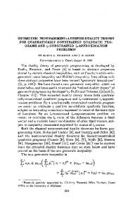
Two-stage op-amp considered herein.

ysis, …) are due to the formulation of the design problem as a convex optimization problem. Geometric programming (when reformulated as described in Section II-A) is just a special type of convex optimization problem. Although general convex problems can be solved efficiently, the special structure of geometric programming can be exploited to obtain an even more efficient solution algorithm. The method we present can be applied to a wide variety of amplifier architectures, but in this paper, we apply the method to a specific two-stage CMOS op-amp. The authors show how the method extends to other architectures in [49] and [50]. A longer version of this paper, which includes more detail about the models, some of the derivations, and SPICE simulation parameters, is available at the authors’ web site [51]. Related work has been reported in several conference publications, e.g., [48]–[50]. A. The Two-Stage Amplifier The specific two-stage CMOS op-amp we consider is shown in Fig. 1. The circuit consists of an input differential stage with active load followed by a common-source stage also with active load. An output buffer is not used; this amplifier is assumed to be part of a very large scale integration (VLSI) system and is only required to drive a fixed on-chip capacitive load of a few picofarads. This op-amp architecture has many advantages: high open-loop voltage gain, rail-to-rail output swing, large common-mode input range, only one frequency compensation capacitor, and a small number of transistors. Its main drawback is the nondominant pole formed by the load capacitance and the output impedance of the second stage, which reduces the achievable bandwidth. Another potential disadvantage is the right half-plane zero that arises from the feedforward signal path through the compensating capacitor. Fortunately, the zero is easily removed by a suitable choice for the compensation (see [2]). resistor This op-amp is a widely used general purpose op-amp [88]; it finds applications, for example, in switched capacitor filters [23], analog-to-digital converters [60], [72], and sensing circuits [85]. There are 18 design parameters for the two-stage op-amp: • The widths and lengths of all transistors, i.e., and .

There is a huge literature, which goes back more than 20 years, on computer-aided design (CAD) of analog circuits. A good survey of early research can be found in the survey [11]; more recent papers on analog-circuit CAD tools include [4], [12], [13]. The problem we consider in this paper, i.e., selection of component values and transistor dimensions, is only a part of a complete analog-circuit CAD tool. Other parts, which we do not consider here, include topology selection (see [66]) and actual circuit layout (see, e.g., ILAC [27], KOAN/ANAGRAM II [15]). The part of the CAD process that we consider lies between these two tasks; the remainder of the discussion is restricted to methods dealing with component and transistor sizing. 1) Classical Optimization Methods: General-purpose classical optimization methods, such as steepest descent, sequential quadratic programming, and Lagrange multiplier methods, have been widely used in analog-circuit CAD. These methods can be traced back to the survey paper [11]. The widely used general-purpose optimization codes NPSOL [39] and MINOS [71] are used in [25], [64], and [67]. LANCELOT [16], another general-purpose optimizer, is used in [22]. Other CAD approaches based on classical optimization methods, and extensions such as a minimax formulation, include the one described in [47], [61], and [63], OAC [78], OPASYN [56], CADICS [54], WATOPT [31], and STAIC [45]. The classical methods can be used with more complicated circuit models, including even full SPICE simulations in each iteration, as in DELIGHT.SPICE [75] (which uses the general-purpose optimizer DELIGHT [76]) and ECSTASY [86]. The main advantage of these methods is the wide variety of problems they can handle; the only requirement is that the performance measures, along with one or more derivatives, can be computed. The main disadvantage of the classical optimization methods is they only find locally optimal designs. This means that the design is at least as good as neighboring designs, i.e., small variations of any of the design parameters results in a worse (or infeasible) design. Unfortunately this does not mean the design is the best that can be achieved, i.e., globally optimal; it is possible (and often happens) that some other set of design parameters, far away from the one found, is better. The same problem arises in determining feasibility: a classical (local) optimization method can fail to find a feasible design, even though one exists. Roughly speaking, classical methods can get stuck at local minima. This shortcoming is so well known that it is often not even mentioned in papers; it is taken as understood. The problem of nonglobal solutions from classical optimization methods can be treated in several ways. The usual approach

DEL MAR HERSHENSON et al.: OPTIMAL DESIGN OF A CMOS OP-AMP VIA GEOMETRIC PROGRAMMING

is to start the minimization method from many different initial designs, and to take the best final design found. Of course, there are no guarantees that the globally optimal design has been found; this method merely increases the likelihood of finding the globally optimal design. This method also destroys one of the advantages of classical methods, i.e., speed, since the computation effort is multiplied by the number of different initials designs that are tried. This method also requires human intervention (to give “good” initial designs), which makes the method less automated. The classical methods become slow if complex models are used, as in DELIGHT.SPICE, which requires more than a complete SPICE run at each iteration (“more than” since, at the least, gradients must also be computed). 2) Knowledge-Based Methods: Knowledge-based and expert-systems methods have also been widely used in analog circuit CAD. Examples include genetic algorithms or evolution systems like SEAS [74], DARWIN [58], [100]; systems based on fuzzy logic like FASY [46] and [92]; special heuristics-based systems like IDAC [29], [30], OASYS [44], BLADES [21], and KANSYS [43]. One advantage of these methods is that there are few limitations on the types of problems, specifications, and performance measures that can be considered. Indeed, there are even fewer limitations than for classical optimization methods since many of these methods do not require the computation of derivatives. These methods have several disadvantages. They find a locally optimal design (or, even just a “good” or “reasonable” design) instead of a globally optimal design. The final design depends on the initial design chosen and the algorithm parameters. As with classical optimization methods, infeasibility is not unambiguously detected; the method simply fails to find a feasible design (even when one may exist). These methods require substantial human intervention either during the design process, or during the training process. 3) Global Optimization Methods: Optimization methods that are guaranteed to find the globally optimal design have also been used in analog-circuit design. The most widely known global optimization methods are branch and bound [103] and simulated annealing [94], [101]. A branch and bound method is used, e.g., in [66]. Branch and bound methods unambiguously determine the globally optimal design: at each iteration they maintain a suboptimal feasible design and also a lower bound on the achievable performance. This enables the algorithm to terminate nonheuristically, i.e., with complete confidence that the global design has been found within a given tolerance. The disadvantage of branch and bound methods is that they are extremely slow, with computation growing exponentially with problem size. Even problems with 10 variables can be extremely challenging. Simulated annealing (SA) is another very popular method that can avoid becoming trapped in a locally optimal design. In principle it can compute the globally optimal solution, but in implementations there is no guarantee at all, since, for example, the cooling schedules called for in the theoretical treatments are not used in practice. Moreover, no real-time lower bound is available, so termination is heuristic. Like classical and knowledge-based methods, SA allows a very wide variety

3

of performance measures and objectives to be handled. Indeed, SA is extremely effective for problems involving continuous variables and discrete variables, as in, e.g., simultaneous amplifier topology and sizing problems. SA has been used in several tools such as ASTR/OBLX [77], OPTIMAN [38], FRIDGE [68], SAMM [105], and [14]. The main advantages of SA are that it handles discrete variables well, and greatly reduces the chances of finding a nonglobally optimal design. (Practical implementations do not reduce the chance to zero, however.) The main disadvantage is that it can be very slow, and cannot (in practice) guarantee a globally optimal solution. 4) Convex Optimization and Geometric Programming Methods: In this section, we describe the general optimization method we employ in this paper: convex optimization. These are special optimization problems in which the objective and constraint functions are all convex. While the theoretical properties of convex optimization problems have been appreciated for many years, the advantages in practice are only beginning to be appreciated now. The main reason is the development of extremely powerful interior-point methods for general convex optimization problems in the last five years (e.g., [73] and [102]). These methods can solve large problems, with thousands of variables and tens of thousands of constraints, very efficiently (in minutes on a small workstation). Problems involving tens of variables and hundreds of constraints (such as the ones we encounter in this paper) are considered small, and can be solved on a small current workstation in less than one second. The extreme efficiency of these methods is one of their great advantages. The other main advantage is that the methods are truly global, i.e., the global solution is always found, regardless of the starting point (which, indeed, need not be feasible). Infeasibility is unambiguously detected, i.e., if the methods do not produce a feasible point they produce a certificate that proves the problem is infeasible. Also, the stopping criteria are completely nonheuristic: at each iteration a lower bound on the achievable performance is given. One of the disadvantages is that the types of problems, performance specifications, and objectives that can be handled are far more restricted than any of the methods described above. This is the price that is paid for the advantages of extreme efficiency and global solutions. (For more on convex optimization, and the implications for engineering design, see [10].) The contribution of this paper is to show how to formulate the analog amplifier design problem as a certain type of convex problem called geometric programming. The advantages, compared to the approaches described above, are extreme efficiency and global optimality. The disadvantage is less flexibility in the types of constraints we can handle, and the types of circuit models we can employ. Aside from work we describe below, the only other application of geometric programming to circuit design is in transistor and wire sizing for Elmore delay minimization in digital circuits, as in TILOS [36] and other programs [81], [82], [87]. Their use of geometric programming can be distinguished from ours in several ways. First of all, the geometric programs that arise in Elmore delay minimization are very specialized (the

4


only exponents that arise are 0 and ). Second, the problems they encounter in practice are extremely large, involving up to hundreds of thousands of variables. Third, their representation of the problem as a geometric program is quite an approximation, since the actual circuits are nonlinear, and the threshold delay, not Elmore delay, is the true objective. Convex optimization is mentioned in several papers on analog-circuit CAD. The advantages of convex optimization are mentioned in [65] and [66]. In [25] and [26], the authors use a supporting hyperplane method, which they point out provides the global optimum if the feasible set is convex. In [89], the authors optimize a few design variables in an op-amp using a Lagrange multiplier method, which yields the global optimum since the small subproblems considered are convex. In [95] and [96], convex optimization is used to optimize area, power, and dominant time constant in digital circuit wire and transistor sizing. During the review process for this paper, the authors were informed of similar work that had been submitted to IEEE TRANSACTIONS ON COMPUTER-AIDED DESIGN OF INTEGRATED CIRCUITS AND SYSTEMS by Mandal and Visvanathan [24]. Mandal and Visvanathan show how geometric programming can be used to size another simple op-amp, and describe a simple method for iteratively refining monomial device models. C. Outline of Paper In Section II, we briefly describe geometric programming, the special type of optimization problem at the heart of the method, and show how it can be cast as a convex optimization problem. In Sections III–VI we describe a variety of constraints and performance measures, and show that they have the special form required for geometric programming. In Section VII we give numerical examples of the design method, showing globally optimal tradeoff curves among various performance measures such as bandwidth, power, and area. We also verify some of our designs using high fidelity SPICE models, and briefly discuss how our method can be extended to handle short-channel effects. In Section IX, we discuss robust design, i.e., how to use the methods to ensure proper circuit operation under various processing conditions. In Section X, we give our concluding remarks. II. GEOMETRIC PROGRAMMING Let be real, positive variables. We will denote of these variables as . A function is the vector called a posynomial function of if it has the form

posynomial (but not monomial); is a monomial is nei(and, therefore, also a posynomial); while ther. Note that posynomials are closed under addition, multiplication, and nonnegative scaling. Monomials are closed under multiplication and division. A geometric program is an optimization problem of the form minimize subject to (1) are posynomial functions and are where monomial functions. Several extensions are readily handled. If is a posynomial can and is a monomial, then the constraint (since is be handled by expressing it as posynomial). For example, we can handle constraints of the , where is posynomial and . In a simform ilar way if and are both monomial functions, then we can by expressing it handle the equality constraint (since is monomial). as We will also encounter functions whose reciprocals are is inverse posynomial if is a posynomials. We say posynomial. If is an inverse posynomial and is a posynomial, then geometric programming can handle the constraint by writing it as . As another example, if is an inverse posynomial, then we can maximize . it, by minimizing (the posynomial) Geometric programming has been known and used since the late 1960s, in various fields. There were two early books on geometric programming, by Duffin et al. [18] and Zener [106], which include the basic theory, some electrical engineering applications (e.g., optimal transformer design), but not much on numerical solution methods. Another book appeared in 1976 [9]. The 1980 survey paper by Ecker [19] has many references on applications and methods, including numerical solution methods used at that time. Geometric programming is briefly described in some surveys of optimization, e.g., [20, pp. 326–328] or [99, Ch. 4]. While geometric programming is certainly known, it is nowhere near as widely known as, say, linear programming. In addition, advances in general-purpose nonlinear constrained optimization algorithms and codes (such as the ones described above) have contributed to decreased use (and knowledge) of geometric programming in recent years. A. Geometric Programming in Convex Form

where and . Note that the coefficients must can be any real numbe nonnegative, but the exponents bers, including negative or fractional. When there is exactly one and , we call a nonzero term in the sum, i.e., monomial function. (This terminology is not consistent with the standard definition of a monomial in algebra, but it should not is cause any confusion.) Thus, for example,

A geometric program can be reformulated as a convex optimization problem, i.e., the problem of minimizing a convex function subject to convex inequality constraints and linear equality constraints. This is the key to our ability to globally and efficiently solve geometric programs. We define new variables , and take the logarithm of a posynomial to get


where and . It can be shown that is a convex function of the new variable : for all and we have

Note that if the posynomial is a monomial, then the transformed function is affine, i.e., a linear function plus a constant. We can convert the standard geometric program (1) into a convex program by expressing it as

5

ciency. Problems with hundreds of variables and thousands of constraints are readily handled, on a small workstation, in minutes; the problems we encounter in this paper, which have on the order of ten variables and 100 constraints, are easily solved in under one second. To carry out the designs in this paper, we implemented, in MATLAB, a simple and crude primal barrier method for solving the convex form problem. Roughly speaking, this method consists of applying a modified Newton’s method to minimizing the smooth convex function

minimize subject to (2) This is the so-called convex form of the geometric program (1). Convexity of the convex form geometric program (2) has several important implications: we can use efficient interior-point methods to solve them, and there is a complete and useful duality, or sensitivity theory for them; see, e.g., [10]. B. Solving Geometric Programs Since Ecker’s survey paper, there have been several important developments, related to solving geometric programming in the convex form. A huge improvement in computational efficiency was achieved in 1994, when Nesterov and Nemirovsky developed efficient interior-point algorithms to solve a variety of nonlinear optimization problems, including geometric programs [73]. Recently, Kortanek et al. have shown how the most sophisticated primal-dual interior-point methods used in linear programming can be extended to geometric programming, resulting in an algorithm approaching the efficiency of current interior-point linear programming solvers [57]. The algorithm they describe has the desirable feature of exploiting sparsity in the problem, i.e., efficiently handling problems in which each variable appears in only a few constraints. Other methods developed specifically for geometric programs include those described by Avriel et al. [7] and Rajpogal and Bricker [80], which require solving a sequence of linear programs (for which very efficient algorithms are known). The algorithms described above are specially tailored for the geometric program (in convex form). It is also possible to solve the convex form problem using general purpose optimization codes that handle smooth objectives and constraint functions, e.g., LANCELOT [16], MINOS [71], LOQO [97], or LINGO-NL [83]. These codes will (in principle) find a globally optimal solution, since the convex form problem is convex. They will also determine the optimal dual variables (sensitivities) as a by-product of solving the problem. In an unpublished report [104], Xu compares the performance of the sophisticated primal-dual interior-point method developed by Kortanek et al.(XGP, [57]) with two general-purpose optimizers, MINOS and LINGO-NL, on a suite of standard geometric programming problems (in convex form). The general-purpose codes fail to solve some of the problems, and in all cases take substantially longer to obtain the solution. For our purposes, the most important feature of geometric programs is that they can be globally solved with great effi-

subject to the affine (linear equality) constraints , , for an increasing sequence of values of , starting from the optimal found for , the the last value of . It can be shown that when optimal solution of this problem is no more than suboptimal for the original convex form geometric program (GP). The , computational complexity of this simple method is where is the number of variables, and is the total number of terms in monomials and posynomials in the objective and constraints. For much more detail, see [10] and [35]. Despite the simplicity of the algorithm (i.e., primal only, with no sparsity exploited) and the overhead of an interpreted language, the geometric programs arising in this paper were all solved in approximately 1 or 2 s on an ULTRA SPARC1 running at 170 MHz. Since our simple interior-point method is already extremely fast on the relatively small problems we encounter in this paper, we feel that the choice of algorithm is not critical. When the method is applied to large-scale problems, such as the ones obtained for a robust design problem (see Section IX), the choice may well become critical. C. Sensitivity Analysis Suppose we modify the right-hand sides of the constraints in the geometric program (1) as follows: minimize subject to (3) and are zero, this modified geometric proIf all of the , then the congram coincides with the original one. If represents a tightened version of the origstraint ; conversely if , it repreinal th constraint gives a logasents a loosening of the constraint. Note that rithmic or fractional measure of the change in the specification: means that the th constraint is loosened 10%, means that the th constraint is tightwhereas ened 10%. denote the optimal objective value of the modLet ified geometric program (3), as a function of the parameters and , so the original ob. In sensitivity analysis, we study the jective value is as a function of and , for small and . To variation of

6


express the change in optimal objective function in a fractional form, we use the logarithmic sensitivities

The biasing transistors the same length

,

, and

must match, i.e., have

(4)

(6)

, . These sensitivity numbers are evaluated at dimensionless, since they express fractional changes per fractional change. For simplicity we are assuming here that the original geometric program is feasible, and remains so for small changes in the right-hand sides of the constraints, and also that the optimal objective value is differentiable as a function of and . More complete descriptions of sensitivity analysis in other cases can be found in the references cited above, or in a general context in [10]. The surprising part is that the sensitivity numbers and come for free, when the problem is solved using an interior-point or Lagrangian-based method (from the solution of the dual problem; see [10]). We start with some simple observations. If at the optimal soof the original problem, the th inequality constraint lution is strictly less than one, then is not active, i.e., (since we can slightly tighten or loosen the th constraint with since increasing slightly no effect). We always have loosens the constraints, and hence lowers the optimal objective value. The sign of tells us whether increasing the right-hand increases or decreases side side of the equality constraint the optimal objective value. The sensitivity numbers are extremely useful in practice, and give tremendous insight to the designer. Suppose, for example, is power dissipation, reprethat the objective sents the constraint that the bandwidth is at least 30 MHz, and represents the constraint that the open-loop gain is V V. Then , say, tells us that a small fractional increase in required bandwidth will translate into a three times tells larger fractional increase in power dissipation. us that a small fractional increase in required open-loop gain will translate into a fractional increase in power dissipation only one-tenth as big. Although both constraints are active, the sensitivities tell us that the design is, roughly speaking, more tightly constrained by the bandwidth constraint than the open-loop gain constraint. The sensitivity information from the example above might lead the designer to reduce the required bandwidth (to reduce power), or perhaps increase the open-loop gain (since it would not cost much). We give an example of sensitivity analysis in Section VII-D.

The six equality constraints in (5) and (6) have monomial expressions on the left- and right-hand sides and hence, are readily handled in geometric programming (by expressing ). them as monomial equality constraints such as Note that (5) and (6) effectively reduce the number of variables from 18 to 12. We can, for example, eliminate the variables and by substituting wherever they appear. For clarity, and in our discuswe will continue to use the variables sion; for computational purposes, however, they can be replaced by . (In any case, the number of variables and constraints is so small for a geometric program that there is almost no computational penalty in keeping the extra variables and equality constraints.)

III. DIMENSION CONSTRAINTS We start by considering some very basic constraints involving the device dimensions, e.g., symmetry, matching, minimum or maximum dimensions, and area limits. A. Symmetry and Matching For the intended operation of the input differential pair, tranand must be identical and transistors and sistors must also be identical. These conditions translate into the four equality constraints (5)

B. Limits on Device Sizes Lithography limitations and layout rules impose minimum (and possibly maximum) sizes on the transistors

(7) These 32 constraints can be expressed as posynomial constraints , etc. Since and are variables such as (hence, monomials), we can also fix certain devices sizes, i.e., impose equality constraints. We should note that a constraint limiting device dimensions to a finite number of allowed values, or to an integer multiple of some fixed small value, cannot be (directly) handled by geometric programming. Such constraints can be approximately handled by simple rounding to an allowed value, or using more sophisticated mixed convex-integer programming methods. C. Area The op-amp die area can be approximated as a constant plus the sum of transistor and capacitor area as (8) gives the fixed area, is the ratio of capacitor Here (if it is not one) area to capacitance, and the constant can take into account wiring in the drain and source area. This expression for the area is a posynomial function of the design parameters, so we can impose an upper bound on the area, i.e., , or use the area as the objective to be minimized. This simple expresion does not take routing area into account; more accurate posynomial formulas for the amplifier die area could be developed, if needed. D. Systematic Input Offset Voltage and To reduce input offset voltage, the drain voltages of must be equal, ensuring that the current is split equally


between transistors and , , and densities of

. This happens when the current are equal, i.e., (9)

are each posynomial inequalities on the design variables and, hence, can be handled by geometric programming. • Transistor . The lowest common-mode input voltage imposes the toughest constraint on transistor remaining in saturation. The condition is

These two conditions are equality constraints between monomials, and are therefore readily handled by geometric programming. IV. BIAS, CONDITIONS, SIGNAL SWING, CONSTRAINTS

AND

(12)

POWER

In this section, we consider constraints involving bias conditions, including the effects of common-mode input voltage and output signal swing. We also consider the quiescent power of the op-amp (which is determined, of course, by the bias conditions). In deriving these constraints, we assume that the symmetry and matching conditions (5) and (6) hold. To derive the equations, we use a standard long-channel square-law model for the MOS transistors, which is described in detail in the Appendix. We refer to this model as the GP0 model; the same analysis also applies to the more accurate GP1 model, also described in the Appendix. In order to simplify the equations, it is convenient to define , , and the bias currents , , and through transistors , respectively. Transistors and form a current mirror . Their currents are given by with transistor

7

•

• •

•

Note that if the right-hand side of (12) were negative, i.e., , then the design is immeif diately known to be infeasible (since the left-hand side is, of course, positive). . The systematic offset condition (9) makes Transistor equal to the drain voltage of . the drain voltage of being saturated is the Therefore, the condition for being saturated, i.e., (12). same as the condition for is deNote that the minimum allowable value of and entering the linear region. termined by . Since transistor is always Transistor in saturation and no additional constraint is necessary. . The systematic offset condition also imTransistor is equal to the drain plies that the drain voltage of . Thus, will be saturated as well. voltage of . The highest common-mode input voltage Transistor , imposes the tightest constraint on transistor being in saturation. The condition is

(10) Thus and are monomials in the design variables. The curis split equally between transistor rent through transistor and . Thus, we have (11) which is another monomial. Since these bias currents are monomials, we can include lower or upper bounds on them, or even equality constraints, if in order to express other we wish. We will use , , and constraints, remembering that these bias currents can simply be eliminated (i.e., expressed directly in terms of the design variables) using (10) and (11). A. Bias Conditions The setup for deriving the bias conditions is as follows. The input terminals are at the same dc potential, the common-mode . We assume that the common-mode input input voltage voltage is allowed to range between a minimum value and a maximum value , which are given. Similarly, we assume that the output voltage is allowed to swing between and a maximum value a minimum value (which takes into account large signal swings in the output). The bias conditions are that each transistor should remain in saturation for all possible values of the input common-mode voltage and the output voltage. The derivation of the bias constraints given below can be found in the longer report [51]. The important point here is that the constraints

(13) is deThus, the maximum allowable value of entering the linear region. As explained termined by above, if the right-hand side of (13) is negative, i.e., , then the design is obviously infeasible. . The most stringent condition occurs when • Transistor the output voltage is at its minimum value (14) In this case the right-hand side of (14) will not be negative if we assume the minimum output voltage is above the negative supply voltage. . For , the most stringent condition oc• Transistor curs when the output voltage is at its maximum value

(15) Here too, the right hand-side of (15) will be positive assuming the maximum output voltage is below the positive supply voltage. . Since , transistor is always • Transistor in saturation; no additional constraint is necessary.

8


In summary, the requirement that all transistors remain in saturation for all values of common-mode input voltage beand , and all values of output voltage tween and , is given by the four inequalities between (12)–(15). These are complicated, but posynomial constraints on the design parameters.

thors [32], [53], [88]. The compensation scheme has also been analyzed previously, e.g., in [2]. • The open-loop voltage gain is

(20)

B. Gate Overdrive It is sometimes desirable to operate the transistors with a minimum gate overdrive voltage. This ensures that they operate away from the subthreshold region, and also improves matching between transistors. For any given transistor this constraint can be expressed as (16) The expression on the left is a monomial, so we can also impose an upper bound on it, or an equality constraint, if we wish. (We will see in Section IX that robustness to process variations can be dealt with in a more direct way.)

which is monomial function of the design parameters. • The dominant pole is accurately given by (21) and are monomials, and is a design variSince able, is a monomial function of the design variables. is given by • The output pole (22) where , the capacitance at the gate of pressed as

C. Quiescent Power

, can be ex(23)

The quiescent power of the op-amp is given by (17) which is a posynomial function of the design parameters. Hence, we can impose an upper bound on or use it as the objective to be minimized. V. SMALL–SIGNAL TRANSFER FUNCTION CONSTRAINTS A. Small-Signal Transfer Function We now assume that the symmetry, matching, and bias constraints are satisfied, and consider the (small-signal) transfer from a differential input source to the output. To function derive the transfer function , we use a standard small-signal model for the transistors, which is described in the Appendix, Section B. The standard value of the compensation resistor is used, i.e., (18) (see [2]). The transfer function can be well approximated by a four-pole form

(19) is the open-loop voltage gain, is the dominant Here, is the output pole, is the mirror pole, and is pole, the pole arising from the compensation circuit. In order to sim, plify the discussion in the sequel, we will refer to which are positive, as the poles (whereas precisely speaking, the ). poles are We now give the expressions for the gain and poles. The two-stage op-amp has been previously analyzed by many au-

, the total capacitance at the output node, can be and expressed as (24) The meanings of these parameters, and their dependence on the design variables, is given in the Appendix, Secis an inverse tion B. The important point here is that posynomial function of the design parameters (i.e., is a posynomial). is given by • The mirror pole (25) where , the capacitance at the gate of pressed as

, can be ex(26)

is also an inverse posynomial. Thus, • The compensation pole is (27) which is also inverse posynomial. and the dominant pole In summary: the open-loop gain are monomial, and the parasitic poles , , and are all inverse posynomials. Now we turn to various design constraints and specifications that involve the transfer function. B. Open-Loop Gain Constraints is a monomial, we can constrain Since the open-loop gain . We could also impose upper it to equal some desired value or lower bounds on the gain, as in (28)


where and are given lower and upper limits on acceptable open-loop gain. C. Minimum Gain at a Frequency The magnitude squared of the transfer function at a frequency is given by

Since are all inverse posynomial, the expressions are posynomial. Hence, the whole denominator is posynomial. The numerator is monomial, thus we conclude that the squared mag, is inverse posynonitude of the transfer function, mial. (Indeed, it is inverse posynomial in the design variables as well.) We can, therefore, impose any constraint of the and form

using

geometric

programming [by ]. The transfer function magnitude creases (since it has only poles), so to for

expressing

it

as

decreases as inis equivalent (29)

We will see below that this allows us to specify a minimum bandwidth or crossover frequency. D. 3-dB Bandwidth is the frequency at which the gain The 3-dB bandwidth drops 3 dB below the dc open-loop gain, i.e., . To specify that the 3-dB bandwidth is at least some , i.e., , is equivalent minimum value . This is turn can be to specifying that expressed as (30) which is a posynomial inequality. In almost all designs will be the dominant pole, (see below) so the 3-dB bandwidth is very accurately given by (31) which is a monomial. Using this (extremely accurate) approximation, we can constrain the 3-dB bandwidth to equal some required value. Using the constraint (30), which is exact but inverse posynomial, we can constrain the 3-dB bandwidth to exceed a given minimum value. E. Dominant Pole Conditions The amplifier is intended to operate with as the dominant pole, i.e., much smaller than , , and . These conditions can be expressed as (32)

9

where we (arbitrarily) use one decade, i.e., a factor of ten in frequency, as the condition for dominance. These dominant pole conditions are readily handled by geometric programming, since is monomial and , , and are all inverse posynomial. In fact these dominant pole conditions usually do not need to be included explicitly since the phase margin conditions described below are generally more strict, and describe the real design constraint. Nevertheless, it is common practice to impose a minimum ratio between the dominant and nondominant poles; see, e.g., [42]. F. Unity-Gain Bandwidth and Phase Margin as the frequency at We define the unity-gain bandwidth . The phase margin is defined in terms of which the phase of the transfer function at the unity-gain bandwidth PM A phase margin constraint specifies a lower bound on the phase – . margin, typically between The unity-gain bandwidth and phase margin are related to the closed-loop bandwidth and stability of the amplifier with unity-gain feedback, i.e., when its output is connected to the inverting input. If the op-amp is to be used in some other specific closed-loop configuration, then a different frequency will be of more interest, but the analysis is the same. For example, if the op-amp is to be used in a feedback configuration dB, then the critical frequency is with closed-loop gain the 20-dB crossover point, i.e., the frequency at which the open-loop gain drops to 20 dB, and the phase margin is defined at that frequency. All of the analysis below is readily adapted with minimal changes to such a situation. For simplicity, we continue the discussion for the unity-gain bandwidth. We start by considering a constraint that the unity-gain bandwidth should exceed a given minimum frequency, i.e., (33) This constraint is just a minimum gain constraint at the fre[as in (29)], and, thus, can be handled exactly quency by geometric programming as a posynomial inequality. Here too we can develop an approximate expression for the unity-gain bandwidth which is monomial. If we assume the parasitic poles , , and are at least a bit (say, an octave) above the unity-gain bandwidth, then the unity-gain bandwidth can be approximated as the open-loop gain times the 3-dB bandwidth, i.e., (34) which is a monomial. If we use this approximate expression for the unity-gain bandwidth, we can fix the unity-gain bandwidth at a desired value. The approximation (34) ignores the decrease in gain due to the parasitic poles and, consequently, overestimates the actual unity-gain bandwidth (i.e., the gain drops to ). 0 dB at a frequency slightly less than We now turn to the phase margin constraint, for which we can give a very accurate posynomial approximation. Assuming the

10


open-loop gain exceeds ten or so, the phase contributed by the , dominant pole at the unity-gain bandwidth, i.e., . Therefore, the phase margin constraint will be very nearly can be expressed as PM

(35)

i.e., the nondominant poles cannot contribute more than PM total phase shift. The phase margin constraint (35) cannot be exactly handled by geometric programming, so we use two reasonable approximations to form a posynomial approximation. The first is an ap[from (34)] instead proximate unity-gain bandwidth as the frequency at which of the exact unity-gain bandwidth we will constrain the phase of . As mentioned above, we have , thus, our specification is a bit stronger than the exact phase margin specification (since we are constraining the phase at a frequency slightly above the actual unity gain bandas a monomial. width). We will also approximate , which is A simple approximation is given by less than . Thus, assuming that quite accurate for each of the parasitic poles contributes no more than about of phase shift, we can approximate the phase margin constraint accurately as PM

(36)

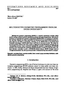
which is a posynomial inequality in the design variables (since is monomial). The approximation error involved here is almost always very small for the following reasons. The constraint (36) makes sure none of the nondominant poles is too near . This, in turn, validates our approximation . It also ensures that our approximation that the phase conis good. tributed by the nondominant poles is Finally, we note that it is possible to obtain a more accurate that has less error over monomial approximation of . For example the approxia wider range, e.g., gives a fit around for angles mation between 0– , as shown in Fig. 2. VI. OTHER CONSTRAINTS In this section, we collect several other important constraints. A. Slew Rate The slew rate can be expressed [79] as SR

Fig. 2.

Approximations of arctan(x).

B. Common-Mode Rejection Ratio The common-mode rejection ratio (CMRR) can be approximated as CMRR C

(38)

which is a monomial. In particular, we can specify a minimum acceptable value of CMRR. C. Power-Supply Rejection Ratio 1) Negative Power-Supply Rejection Ratio: The negative power-supply rejection ratio (PSRR) is given by [52], [59] (39) Thus, the low-frequency negative PSRR is given by the inverse posynomial expression (40) which, therefore, can be lower bounded. The high-frequency PSRR characteristics are generally more critical than the low-frequency PSRR characteristics since noise in mixed-mode chips (clock noise, switching regulator noise, etc.) is typically high frequency. One can see that the expression for the magnitude squared of the negative PSRR at a frequency has the form PSRR

In order to ensure a minimum slew-rate SR the two constraints SR These two constraints are posynomial.

we can impose

SR

(37)

where , , and are given by inverse posynomial expressions. As in Section V-C, we can impose a lower bound on the negative PSRR at frequencies smaller than the unity-gain bandwidth by imposing posynomial constraints of the form PSRR

(41)


2) Positive Power-Supply Rejection Ratio: The low-frequency positive PSRR is given by PSRR

11

TABLE I DESIGN CONSTRAINTS AND SPECIFICATIONS FOR THE TWO-STAGE OP-AMP

(42)

which is neither posynomial nor inverse-posynomial, thus, it follows that constraints on the positive power supply rejection cannot be handled by geometric programming. However, this op-amp suffers from much worse negative PSRR characteristics than positive PSRR characteristics, both at low and high frequencies [40], [42]. Therefore, not constraining the positive PSRR is not critical. We must at the least check the positive PSRR of any design carried out by the method described in this paper. (It is more than adequate in every design we have carried out.) However, if the positive PSRR specification becomes critical, it can be approximated (conservatively) by a posynomial inequality, e.g., using Duffin linearization [7], [17]. D. Noise Performance The equivalent input-referred noise power spectral density (in V /Hz, at frequency assumed smaller than the 3-dB bandwidth), can be expressed as

where is the input-referred noise power spectral density of . These spectral densities consist of the input-retransistor noise ferred thermal noise and a

The total rms noise level over a frequency band (where is below the equivalent noise bandwidth of the circuit) can be found by integrating the noise spectral density:

Therefore, imposing a maximum total rms noise voltage over is the posynomial constraint the band (44)

Thus, the input-referred noise spectral density can be expressed as

(since and are fixed, and design variables).

and

are posynomials in the

VII. OPTIMAL DESIGN PROBLEMS AND EXAMPLES A. Summary of Constraints and Specifications

where

Note that and are (complicated) posynomial functions of the design parameters. We can, therefore, impose spot noise constraints, i.e., require that (43) for a certain , as a posynomial inequality. (We can impose multiple spot noise constraints, at different frequencies, as multiple posynomial inequalities.)

The many performance specifications and constraints described in the previous sections are summarized in Table I. Note that with only one exception (the positive supply rejection ratio), the specifications and constraints can be handled via geometric programming. Since all the op-amp performance measures and constraints shown above can be expressed as posynomial functions and posynomial constraints, we can solve a wide variety of op-amp design problems via geometric programming. We can, for example, maximize the bandwidth subject to given (upper) limits on op-amp power, area, and input offset voltage, and given (lower) limits on transistor lengths and widths, and voltage gain, CMRR, slew rate, phase margin, and output voltage swing. The resulting optimization problem is a geometric programming problem. The problem may appear to be very complex, involving many complicated inequality and equality constraints, but in fact is readily solved.

12


TABLE II SPECIFICATIONS AND CONSTRAINTS FOR DESIGN EXAMPLE

TABLE III OPTIMAL DESIGN FOR DESIGN EXAMPLE

B. Example In this section, we describe a simple design example. A 0.8 m CMOS technology was used; see the longer report [51] for more details and the technology parameters. The positive supply voltage was set at 5 V and the negative supply voltage was set at 0 V. The load capacitance was 3 pF. The objective is to maximize unity-gain bandwidth subject to the requirements shown in Table II. The resulting geometric program has 18 variables, seven (monomial) equality constraints, and 28 (posynomial) inequality constraints. The total number of monomial terms appearing in the objective and all constraints is 68. Our simple MATLAB program solves this problem in under one second real-time. The optimal design obtained is shown in Table III. The performance achieved by this design, as predicted by the program, is summarized in Table IV. The design achieves an 86-MHz unity-gain bandwidth. Note that some constraints are tight (minimum device length, minimum device width, maximum output voltage, quiescent power, phase margin and inputreferred spot noise) while some constraints are not tight (area, minimum output voltage open-loop gain, common-mode rejection ratio, and slew rate).

TABLE IV PERFORMANCE OF OPTIMAL DESIGN FOR DESIGN EXAMPLE

C. Tradeoff Analyses By repeatedly solving optimal design problems as we sweep over values of some of the constraint limits, we can sweep out globally optimal tradeoff curves for the op-amp. For example, we can fix all other constraints, and repeatedly minimize power as we vary a minimum required unity-gain bandwidth. The resulting curve shows the globally optimal tradeoff between unity-gain bandwidth and power (for the values of the other limits). In this section, we show several optimal tradeoff curves for the operational amplifier. We do this by fixing all the specifications at the default values shown in Table II, except two that we vary to see the effect on a circuit performance measure. When the optimization objective is not bandwidth we use a default value of minimum unity-gain bandwidth of 30 MHz. We first obtain the globally optimal tradeoff curve of unity-gain bandwidth versus power for different supply voltages. The results can be seen in Fig. 3. Obviously the more power we allocate to the amplifier, the larger the bandwidth obtained; the plots, however, show exactly how much more bandwidth we can obtain with different power budgets. We can see, for example, that the benefits of allocating more power to the op-amp disappear above 5 mW for a supply voltage of 2.5 V, whereas for a 5 V supply the bandwidth continues to increase with increasing power. Note also that each of the supply voltages gives the largest unity-gain bandwidth over some range of powers. In Fig. 4, we plot the globally optimal tradeoff curve of open-loop gain versus unity-gain frequency for different phase margins. Note that for a large unity-gain bandwidth requirement only small gains are achievable. Also, we can see that for a tighter phase margin constraint the gain bandwidth product is lower. Fig. 5 shows the minimum input-referred spectral density at 1 kHz versus power, for different unity-gain frequency requirements. Note that when the power specification is tight, increasing the power greatly helps to decrease the input-referred noise spectral density. In Fig. 6 we show the optimal tradeoff curve of unity-gain bandwidth versus area for different different power budgets.


13

Fig. 3. Maximum unity-gain bandwidth versus power for different supply voltages.

Fig. 5. Minimum noise density at 1 kHz versus power for different unity-gain bandwidths.

Fig. 4. Maximum open-loop gain versus unity-gain bandwidth for different phase margins.

Fig. 6. Maximum unity-gain bandwidth versus area for different power budgets.

We can see that when the area constraint is tight, increasing the available area translates into a greater unity bandwidth. After some point, other constraints become more stringent and increasing the available area does not improve the maximum achievable unity-gain bandwidth. Several other optimal tradeoff curves are given in the longer report [51].

There are six active constraints: minimum device length, minimum device width, maximum output voltage, quiescent power, phase margin, and input-referred spot noise at 1 kHz. All of these constraints limit the maximum unity-gain bandwidth. The sensitivities indicate which of these constraints are more critical (more limiting). For example, a 10% increase in the allowable input-referred noise at 1 kHz will produce a design with (approximately) 2.4% improvement in unity-gain bandwidth. However, a 10% decrease in the maximum phase margin at the unity-gain bandwidth will produce a design with (approximately) 17.6% improvement in unity-gain bandwidth. It is very interesting to analyze the sensitivity to the minimum device width constraint. A 10% decrease in the minimum device width produces a design with only a 0.05% improvement in unity-gain bandwidth. This can be interpreted as follows: even though the minimum device width constraint is binding, it can be considered not binding in a practical sense since tightening (or loosening) it will barely change the objective. The program classifies the given constraints in order of importance from most limiting to least limiting. For this design

D. Sensitivity Analysis Example In this section, we analyze the information provided by the sensitivity analysis of the first design problem in Section VII-B (maximize the unity-gain bandwidth when the rest of specifications/constraints are set to the values shown in Table II). The results of this sensitivity analysis are shown in Table V. The column labeled “Sensitivity” (numerical) is obtained by tightening and loosening the constraint in question by 5% and resolving the problem. (The average from the two is taken.) The column labeled “Sensitivity” comes (essentially for free) from solving the original problem. Note that it gives an excellent prediction of the numerically obtained sensitivities.

14


TABLE V SENSITIVITY ANALYSIS FOR THE DESIGN EXAMPLE

TABLE VI DESIGN VERIFICATION WITH HSPICE LEVEL-1. THE PERFORMANCE MEASURES OBTAINED BY THE PROGRAM ARE COMPARED WITH THOSE FOUND BY HSPICE LEVEL 1 SIMULATION

the order is: phase margin, quiescent power, maximum output voltage, minimum device length, input-referred noise at 1 kHz, and minimum device width. The program also tells the designer which constraints are not critical (the ones whose sensitivities are zero or small). A small relaxation of these constraints will not improve the objective function, so any effort to loosen them will not be rewarded.

nonposynomial) HSPICE level-1 model. As an example, Table VI summarizes the results for the standard problem described above in Section VII-D. Note that the values of the performance specifications from the posynomial model (in the column labeled “Program”) and the values according to HSPICE level 1 (in the right-hand side column) are in close agreement. Moreover, the deviations between the two are readily understood. The unity-gain frequency is slightly overestimated and the phase margin is slightly underestimated because we use the approximate expression (34), which ignores the effect of the parasitic poles on the crossover frequency. The noise is overestimated 7% because the open-loop gain has decreased 7% already at 1 kHz; this gain reduction translates into a reduction in the input-referred noise. We have verified the geometric program results with the HSPICE level-1 model simulations for a wide variety of designs (with a wide variety of power, bandwidth, gain, etc.). The results are always in close agreement. Thus, our simple posynomial models are reasonably good approximations of the HSPICE level-1 models.

VIII. DESIGN VERIFICATION Our optimization method is based on GP0 models, which are the simple square-law device models described in the Appendix, Section A. Our model does not include several potentially important factors such as body effect, channel length modulation in the bias equations, and the dependence of junction capacitances on junction voltages. Moreover we make several approximations in the circuit analysis used to formulate the constraints. For example, we approximate the transfer function with the four-pole form (19); the actual transfer function, even based on the simple model, is more complicated. As another example, in our simple version of the we approximate phase margin constraint. While all of these approximations are reasonable (at least when channel lengths are not too short), it is important to verify the designs obtained using a higher fidelity (presumably nonposynomial) model. A. HSPICE Level-1 Verification with GP0 Models We first verify the designs generated by our geometric programming method (using GP0 or long-channel models) with HSPICE using a long-channel model (HSPICE level–1 model). We take the design found by the geometric programming method, and then use the HSPICE level-1 model to check the various performance measures. The level-1 HSPICE model is substantially more accurate (and complicated) than our simple posynomial models. It includes, for example, body effect, channel-length modulation, junction capacitance that depends on bias conditions, and a far more complex transfer function that includes many other parasitic capacitances. The unity gain bandwidth and phase margin are computed by solving the complete small-signal model of the op-amp. The results of such verification always show excellent agreement between our posynomial models and the more complex (and

B. HSPICE BSIM Model Verification with GP1 Models In this section, we show how the geometric programming method performs well even for short-channel devices, when more sophisticated GP1 transistor models are used, by verifying designs against sophisticated HSPICE level-39 (BSIM3v1) simulations. The GP1 model is described in the Appendix, Section B; the only difference is that we use an empirically found monomial expression for the output conductance of a MOS transistor instead of the standard long channel formula. Using these GP1 models, all of the constraints described above are still compatible with geometric programming. Table VII shows the comparison between the results of geometric programming design, using GP1 models, and HSPICE level-39 simulation, for the standard problem described in Section VII-D. The predicted values are very close to the simulated values. The agreement holds for a wide variety of designs. IX. DESIGN FOR PROCESS ROBUSTNESS Thus far, we have assumed that parameters such as transistor threshold voltages, mobilities, oxide parameters, channel modulation parameters, supply voltages, and load capacitance are


TABLE VII DESIGN VERIFICATIONS WITH HSPICE LEVEL-39. GEOMETRIC PROGRAMMING IS USED TO SOLVE THE STANDARD PROBLEM, USING THE MORE SOPHISTICATED GP1 MODELS. THE RESULTS ARE COMPARED WITH HSPICE LEVEL-39 SIMULATION

15

We do not have to give every possible combination of parameter values, but only the ones likely to actually occur. For example, if it is unlikely that the oxide capacitance parameter is at its maximum value while the -threshold voltage is maximum, then we delete these combinations from our set . In this way, we can model interdependencies among the parameter values. We can also construct in a straightforward way. Suppose we require a design that works, without modification, on several processes, or several variations of processes. is then simply a list of the process parameters for each of the processes. The robust design is achieved by solving the problem minimize subject to

all known and fixed. In this section, we show to how to use the methods of this paper to develop designs that are robust with respect to variations in these parameters, i.e., designs that meet a set of specifications for a set of values of these parameters. Such designs can dramatically increase yield. There are many approaches to the problem of robustness and yield optimization (see [5], [28]). The robust design problem can be formulated as a so-called semi-infinite programming problem, in which the constraints must hold for all values of some parameter that ranges over an interval, as in [75], which used DELIGHT.SPICE to do robust designs, or more recently, Mukherjee et al. [69], who use ASTRX/OBLX. These methods often involve very considerable run times, ranging from minutes to hours. We also formulate the problem as a sampled version of a semi-infinite program. The method is practical only because geometric programming can readily handle problems with many hundreds, or even thousands, or constraints; the computational effort grows approximately linearly with the number of constraints. The basic idea in our approach is to list a set of possible parameters, and to replicate the design constraints for all possible denote a vector of parameters that parameter values. Let may vary. Then the objective and constraint functions can be expressed as functions of (the design parameters) and (which we will call the process parameters, even if some components, e.g., the load capacitance, are not really process parameters):

The functions are all posynomial functions of , for each , and the functions are all monomial functions of , for each . be a (finite) set of possible parameter Let values. Our goal is to determine a design (i.e., ) that works well ). for all possible parameter values (i.e., First we describe several ways the set might be constructed. As a simple example, suppose there are six parameters, which . We might vary independently over intervals sample each interval with three values (e.g., the midpoint and extreme values), and then form every possible combination of . parameter values, which results in

for all for all (45)

This problem can be reformulated as a geometric program with times the number of constraints, and an additional scalar variable [22]: minimize subject to

(46) The solution of (45) [which is the same as the solution of (46)] satisfies the specifications for all possible values of the process parameters. The optimal objective value gives the (globally) optimal minimax design. (It is also possible to take an average value of the objective over process parameters, instead of a worst-case value.) Equality constraints have to be handled carefully. Provided the transistor lengths and widths are not subject to variation, equality constraints among them (e.g., matching and symmetry) are likely not to depend on the process parameter . Other equality constraints, however, can depend on . When we enforce an equality constraint for each value of , the result is (usually) an infeasible problem. For example suppose we specify that the open-loop gain equal exactly 80 dB. Process variation will change the open-loop gain, making it impossible to achieve a design that has an open-loop gain of exactly 80 dB for more than a few process parameter values. The solution to this problem is to convert such specifications into inequalities. We might, for example, change our specification to require that the open-loop gain exceed 80 dB, or require it to be between 80 and 85 dB. Either way the robust problem now has at least a chance of being feasible. It is important to contrast a robust design for a set of process with the optimal designs for parameters each process parameter. The objective value for the robust design is worse (or no better) than the optimal design for each parameter value. This disadvantage is offset by the advantage that the design works for all the process parameter values. As a simple example, suppose we seek a design that can be run on

16


two processes ( and ). We can compare the robust design to the two optimal designs. If the objective achieved by the robust design is not much worse than the two optimal designs, then we have the advantage of a single design that works on two processes. On the other hand if the robust design is much worse (or even infeasible) we may elect to have two versions of the amplifier design, each one optimized for the particular process. Thus far, we have considered the case in which the set is finite. However, in most real cases it is infinite; e.g., individual parameters lie in ranges. We have already indicated above that such situations can be modeled or approximated by sampling the interval. While we believe this will always work in practice, it gives no guarantee, in general, that the design works for all values of the parameter in the given range; it only guarantees performance for the sampled values of the parameters. There are many cases, however, when we can guarantee the performance for a parameter value in an interval. Suppose that is posynomial not just in , but in and the function as well, and that lies in the interval . (We take scalar here for simplicity.) It then suffices to impose the constraint at the endpoints of the interval, i.e.,

for all This is easily proved using convexity of the in the transformed variables. The reader can verify that the constraints described above are , , , , , and the parposynomial in the parameters asitic capacitances. Thus, for these parameters at least, we can handle ranges with no approximation or sampling, by specifying the constraints only at the endpoints. The requirement of robustness is a real practical constraint, and is currently dealt with by many methods. For example, a minimum gate overdrive constraint is sometimes imposed because designs with small gate overdrive tend to be nonrobust. The point of this section is that robustness can be achieved in a more methodical way, which takes into account a more detailed description of the possible uncertainties or parameter variations. The result will be a better design than an ad hoc method for achieving robustness. Finally, we demonstrate the method with a simple example. In Table VIII we show how a robust design compares to a nonrobust design. We take three process parameters: the bias current error factor, the positive power supply error factor, and oxide capacitance. The bias current error factor is the ratio of the actual bias current to our design value, so when it is one, the true bias current is what we specify it to be, and when it is 1.1, the true bias current is 10% larger than we specify it to be. Similarly, the positive power supply error factor is the ratio of the actual bias current to our design value. The bias current error factor varies between 0.9–1.1, the positive power supply error factor varies between 0.9–1.1, and the oxide capacitance varies around its nominal value. The three parameters are assumed independent, and we sample each with three values (midpoint and , i.e., 27 difextreme values) so all together we have ferent process parameter vectors. In the third column, we show

TABLE VIII ROBUST DESIGN

the performance of the robust design. For each specification, we determine the worst performance over all 27 process parameters. In the fourth column we show the performance of the nonrobust design. Again, only the worst-case performance over all 27 process parameters is indicated for each specification. The resulting geometric program involves 18 variables, seven monomial equality constraints (i.e., symmetry and matching) and 756 posynomial inequality constraints. The new design obtains a unity-gain bandwidth of 72 MHz. The design in Section VII-B obtains a worst-case unity gain bandwidth of 77 MHz, but since it was specified only for nominal conditions, it fails to meet some constraints when tested over all conditions. For example, the power consumption increases by 15%, the open-loop gain decreases by 20%, the inputreferred spot noise at 1 kHz increases by 5% and the phase margin decreases by . The robust design, on the other hand, meets all specifications for all 27 sets of process parameters. X. DISCUSSION AND CONCLUSION We have shown how geometric programming can be used to design and optimize a common CMOS amplifier. The method yields globally optimal designs, is extremely efficient, and handles a very wide variety of practical constraints. Since no human intervention is required (e.g., to provide an initial “good” design or to interactively guide the optimization process), the method yields completely automated sizing of (globally) optimal CMOS amplifiers, directly from specifications. This implies that the circuit designer can spend more time doing real design, i.e., carefully analyzing the optimal tradeoffs between competing objectives, and less time doing parameter tuning, or wondering whether a certain set of specifications can be achieved. The method could be used, for example, to do full custom design for each op-amp in a complex mixed-signal integrated circuit; each amplifier is optimized for its load capacitance, required bandwidth, closed-loop gain, etc. In fact, the method can handle problems with constraints or coupling between the different op-amps in an integrated circuit. As simple examples, suppose we have 100 op-amps, each with a set of specifications. We can minimize the total area or power by solving a (large) geometric program. In this case, we are solving (exactly) the power/area allocation problem for the 100 op-amps on the integrated circuit. We can also handle direct coupling between the op-amps, i.e., when component values in one op-amp (e.g., input transistor widths) affect another (e.g., as load capacitance). The resulting geometric program will have perhaps hundreds of variables, thousands of constraints, and be


quite sparse, so it is well within the capabilities of current interior-point methods. For example, switched capacitor filters [42] are complex systems where the performance (maximum clock frequency, area, power, etc.) is influenced by both the op-amp and the capacitors. Current CAD tools for switched capacitor filters size the capacitors, but use the same op-amp for all integrators (see, e.g., FIDES [6], [8], [93]). In contrast, we can custom design each op-amp in the switched capacitor filter. Designing optimal op-amps for filters in oversampled converters has also been addressed in [98], but little work has been done to fully automate the design. Limiting amplifiers for FM communication systems [55] require the design of multiple amplifiers in cascade. Typically the same amplifier is used in all stages because it takes too long and it is too difficult to design each stage separately. Our ability to handle much larger problems than arise from a single op-amp design can be used to develop robust designs. This could increase yield, or result in designs with a longer lifetime (since they work with several different processes). The method unambiguously determines feasibility of a set of specifications: it either produces a design that meets the specifications or it provides a proof that the specifications cannot be achieved. In either case it also provides, at essentially no additional cost, the sensitivities with respect to every constraint. This gives a very useful quantitative measure of how tight each constraint is, or how much it affects the objective. In this paper, we have considered only one op-amp circuit, but the general method is applicable to many other circuits, as has been reported in [49] and [50]. For the op-amp considered here, the analytical expressions for the constraints and specifications were derived by hand, but in a more general setting, this step could be partially automated by the use of symbolic circuit simulators like ISAAC [37], SYNAP [84], and ASAP [33]. A CAD tool for optimization of analog op-amps could be developed. It would consist of a symbolic analyzer [34], a GP solver, and a user interface. It could be linked to an automatic layout program, such as ILAC [27] or KOAN/ANAGRAM [15], thus the resulting tool could generate mask designs directly from amplifier specifications. The main disadvantage of the method we have described is that it handles only certain types of constraints and specifications, i.e., monomial equality constraints and posynomial inequality constraints. The main contribution of this paper is to point out that despite this restriction, we can handle a very wide variety of practical amplifier specifications. Another disadvantage of our method, as compared to a more general method, is that the task of formulating the optimization problem for a given circuit topology and set of specifications, requires some user expertise (in circuit design and optimization) and effort. On the other hand, once the formulation is done, particular instances of the design can be carried out automatically and extremely rapidly, by users with no knowledge of the underlying method. The method we propose can be effectively combined with a (local) optimization method that uses nonposynomial, but more accurate model equations or even circuit simulation. Thus, the geometric programming method we propose is used to get close to the (presumably global) optimum, and the final design is tuned using the more accurate (but nonposynomial) model or

17

direct circuit simulation. By iterating between GP-based sizing and parasitic extraction and simulation, we can also address the issue of layout-dependent parasitics by updating the GP models using the extracted parameters. In the many thousands of designs we have carried out, verification with an accurate simulator has shown that our posynomial models are very accurate, thus, presumably, tuning our designs with a more accurate (e.g., simulation-based) method would require only an iteration or two to converge. We close our discussion on the topic of circuit models. This paper has introduced a new quality of a circuit model, i.e., whether it results in posynomial specifications. The traditional tradeoff in circuit modeling is between fidelity and complexity, e.g., simple, but not too accurate models for hand analysis and design, versus complex high fidelity models for design verification. Evidently, we have a third quality for a model: whether or not it results in posynomial specifications. Thus, we have a tradeoff between monomial/posynomial models (for design via GP) and fidelity or accuracy. Note that complexity does not matter: a very complex, but posynomial model is readily handled by GP. Developing accurate, but posynomial circuit models is a new area for research. APPENDIX A. GP0 MOSFET Models Here we describe the MOSFET large- and small-signal models used in our method. The model, which we refer to as GP0, is essentially the standard long-channel square law model described in, [3] and [41]. This model can be inadequate for short-channel transistors [70], [91] in which case better models can be developed that still allow optimization via geometric programming (see the Appendix, Section B). 1) Large-Signal Models: Correct operation of the op-amp requires all transistors to be in saturation. For an NMOS transistor this means (47) When the NMOS transistor is saturated, i.e., (47) holds, the drain current can be expressed as C where transistor channel length; transistor width; electron mobility; oxide capacitance per unit area; C NMOS threshold voltage; channel-length modulation parameter. In developing our bias constraints, we use the simplified large-signal equation C

(48)

i.e., we ignore channel-length modulation. This introduces only a small error.

18


Note that we ignore channel-length modulation in our transconductance expression, but must include it in the output conductance expression (which would otherwise be zero). The gate-to-source capacitance is given by the sum of the gate oxide capacitance and the overlap capacitance C

C

(53)

is the source/drain lateral diffusion length. where The source to bulk capacitance is a junction capacitance and can be expressed as Fig. 7.

Transistor symbols.

(54)

where (55) is the junction built-in potential, and is the source diffusion length. The drain-to-bulk capacitance is also a junction capacitance given by Fig. 8.

Small signal model for a MOSFET.

(56)

For a PMOS transistor, the saturation condition is (49) The drain current is then given by

for equal source and drain diffusions. where The gate-to-drain capacitance is due to the overlap capacitance and is given by C

C where hole mobility; PMOS threshold voltage; channel-length modulation parameter. Here too, we ignore the channel modulation effects and use the simplified expression C

(50)

2) Small-Signal Models: Fig. 8 shows the small-signal model around the operating point for a MOSFET transistor in saturation. The derivation of this model can also be found in [41]. The values of the various elements and parameters are described below. is given by The transconductance C

(51)

(where we ignore, with only small error, channel-length modulation effects). The output conductance is given by (52)

(57)

Equations (53), (55), and (57) are posynomial in the design variables and, therefore, are readily handled. The expressions for the junction capacitances (54) and (56) are not posynomial, and do not depend except in the special case where on the design variables. We can take two approaches to approximating these capacitances. One simple method is to take a worst-case analysis, and use the maximum values (which decreases bandwidth, slew rate, phase margin, etc.) This correor . It is also sponds to the approximation possible to estimate the various junction voltages as constant, so (54) and (56) are constant. In our op-amp circuit, the only junction capacitances that appear in the design equations (see Section V) are the drain-to-bulk , , , , , and . We have escapacitances of , , , timated the drain-to-bulk voltages of transistors , , and , and use these estimated voltages for calculating the junction capacitances. The bulk terminal of the PMOS transistors is connected to and that of the NMOS transistors is the positive supply . The drain voltages connected to the negative supply , , , and are the same as the gate voltage of , of . In most designs, is a few hundred millivolts namely, (recalling that we assume ). Thus, we can above as write (58)


where we use a typical overdrive voltage of The drain-to-bulk capacitances of then given by the expressions

, and

mV. are

19

where again the output conductance is given in millisiemens, the bias current is in milliamps, and the width and length are in micrometers. For all other circuit parameters, we used the GP0 model described above (although we could easily have improved the models using empirical fits to monomials and posynomials). ACKNOWLEDGMENT

The drain voltage of and is the output voltage of the amplifier. The quiescent output voltage is at mid-supply for an as op-amp with small offset. Then, we can write

The authors would like to thank E. Waks, who wrote the geometric programming solver originally used for the numerical experiments shown in this paper. The authors are grateful to B. Fowler, A. E. Gamal, A. Hajimiri, and many anonymous reviewers, for very useful comments and suggestions. REFERENCES

and we obtain constant expressions for

and

These approximations can be validated in several ways. First, we have observed that changing these typical voltages has very little effect on the final designs. And second, SPICE simulation (which includes the junction capacitances) reveals that we incur only small errors. B. GP1 Models The GP0 models described above are essentially the same as the standard long channel device models. It is also possible to derive device models that are more accurate than the long channel models, but at the same time are compatible with geometric programming based design. Analysis of the errors incurred by the GP0 model shows that most of the modeling error comes from the expressions for transconductance and output conductance. By fitting monomial expressions to empirical data, or data obtained from a high-fidelity SPICE simulation, we obtain transistor models that are still compatible with geometric programming-based design. We refer to these models as GP1. We found that the following simple models work very well. For NMOS devices, we use the monomial expression

where the output conductance is given in millisiemens, the bias current is in milliamps, and the width and length are in micrometers. This simple model provides a very good fit over a wide range of transistor width, length, and bias current. For PMOS devices, we find it useful to use two models, one model ) for devices operating at low drain-to-source voltage ( and ) and another one ( ) for devices operating ( , and ) at high drain-to-source voltage ( ,

[1] M. A. Aguirre, J. Chávez, A. Torralba, and L. G. Franquelo, “Analog design optimization by means of a tabu search approach,” in Proc. IEEE Int. Symp. Circuits Syst., vol. 1, 1994, pp. 375–378. [2] B. K. Ahuja, “An improved frequency compensation technique for CMOS operational amplifiers,” IEEE J. Solid-State Circuits, vol. 18, pp. 629–633, Dec. 1983. [3] P. E. Allen and D. R. Holberg, CMOS Analog Circuit Design, 1st ed, U.K.: Oxford, 1987. [4] B. A. A. Antao, “Trends in CAD of analog ICs,” IEEE Circuits Devices Mag., vol. 12, no. 5, pp. 31–41, Sept. 1996. [5] K. J. Antreich and H. E. Graeb, “Circuit optimization driven by worst-case distances,” in Proc. IEEE Int. Conf. Computer-Aided Design, 1991, pp. 166–169. [6] J. Assael, P. Senn, and M. S. Tawfik, “A switched-capapcitor filter silicon compiler,” IEEE J. Solid-State Circuits, vol. 23, pp. 166–174, Feb. 1988. [7] M. Avriel, R. Dembo, and U. Passy, “Solution of generalized geometric programs,” Int. J. Numer. Methods Eng., vol. 9, pp. 149–168, 1975. [8] A. Barlow, K. Takasuka, Y. Nambu, T. Adachi, and J. Konno, “An integrated switched-capacitor filter design system,” in Proc. IEEE Custom Integrated Circuit Conf., 1989, pp. 4.5.1–4.5.5. [9] C. S. Beightler and D. T. Phillips, Applied Geometric Programming. New York: Wiley, 1976. [10] S. Boyd and L. Vandenberghe. (1997) Introduction to convex optimization with engineering applications. Stanford Univ., Stanford, CA. [Online]http://www.stanford.edu/class/ee364/ [11] R. K. Brayton, G. D. Hachtel, and A. Sangiovanni-Vincentelli, “A survey of optimization techniques for integrated-circuit design,” Proc. IEEE, vol. 69, pp. 1334–1362, Oct. 1981. [12] L. R. Carley, G. G. E. Gielen, R. A. Rutenbar, and W. M. C. Sansen, “Synthesis tools for mixed-signal ICs: Progress on front-end and back-end strategies,” in Proc. 33rd Annu. Design Automation Conf., 1996, pp. 298–303. [13] L. R. Carley and R. A. Rutenbar, “How to automate analog IC designs,” IEEE Spectrum, vol. 25, pp. 26–30, Aug. 1988. [14] J. Chávez, M. A. Aguirre, and A. Torralba, “Analog design optimization: A case study,” in Proc. IEEE Int. Symp. Circuits Syst., vol. 3, 1993, pp. 2083–2085. [15] J. M. Cohn, D. J. Garrod, R. A. Rutenbar, and L. R. Carley, “KOAN/ANAGRAM II: New tools for device-placement and routing,” IEEE J. Solid-State Circuits, Mar. 1991. [16] A. R. Conn, N. I. M. Gould, and PH. L. Toint, LANCELOT: A Fortran Package for Large-Scale Nonlinear Optimization (Release A). New York: Springer-Verlag, 1992, vol. 17. [17] R. J. Duffin, “Linearizing geometric programs,” SIAM Rev., vol. 12, pp. 211–227, 1970. [18] R. J. Duffin, E. L. Peterson, and C. Zener, Geometric Programming—Theory and Applications: Wiley, 1967. [19] J. Ecker, “Geometric programming: Methods, computations and applications,” SIAM Rev., vol. 22, no. 3, pp. 338–362, 1980. [20] J. Ecker and M. Kupferschmid, Introduction to Operations Research. Melbourn, FL: Krieger, 1991. [21] F. El-Turky and E. E. Perry, “BLADES: An artificial intelligence approach to analog circuit design,” IEEE Trans. Computer-Aided Design, vol. 8, pp. 680–692, June 1989.

20


[22] A. R. Conn et al., “Optimization of custom CMOS circuits by transistor sizing,” in Proc. IEEE Int. Conf. Computer-Aided Design, 1996, pp. 174–180. [23] D. G. Marsh et al., “A single-chip CMOS PCM codec with filters,” IEEE J. Solid-State Circuits, vol. SC-16, pp. 308–315, Aug. 1981. [24] P. Mandal and V. Visvanathan, “An efficient method of synthesizing CMOS op-amps for globally optimal design,” IEEE Trans. ComputerAided Design, submitted for publication. [25] H. Chang et al., “A top-down constraint-driven design methodology for analog integrated circuits,” in Proc. IEEE Custom Integrated Circuit Conf., 1992, pp. 8.4.1–8.4.6. [26] I. Vassiliou et al., “A video-driver system designed using a top-down, constraint-driven, methodoly,” in Proc. 33rd Annu. Design Automation Conf., 1996. [27] J. Rijmenants et al., “ILAC: An automated layout tool for analog CMOS circuits,” IEEE J. Solid-State Circuits, vol. 24, pp. 417–425, Apr. 1989. [28] J. W. Bandler et al., “Robustizing circuit optimization using Huber functions,” in IEEE MTT-S Int. Microwave Symp. Dig., 1993, pp. 1009–1012. [29] M. G. R. Degrauwe et al., “IDAC: An interactive design tool for analog CMOS circuits,” IEEE J. Solid-State Circuits, vol. SC-22, pp. 1106–1115, Dec. 1987. [30] M. G. R. Degrauwe et al., “Toward an analog system design environment,” IEEE J. Solid-State Circuits, vol. 24, pp. 1587–1597, Dec. 1989. [31] R. Chadha et al., “WATOPT: An optimizer for circuit applications,” IEEE Trans. Computer-Aided Design, vol. CAD-6, pp. 472–479, May 1987. [32] W. C. Black et al., “A high performance low power CMOS channel filter,” IEEE J. Solid-State Circuits, vol. SC-15, pp. 929–938, Dec. 1980. [33] F. V. Fernández, A. Rodríguez-Vázquez, and J. L. Huertas, “Interactive ac modeling and characterization of analog circuits via symbolic analysis,” Analog Integrated Design and Signal Processing, vol. 1, pp. 183–208, Nov. 1991. [34] F. V. Fernández, A. Rodríguez-Vázquez, J. L. Huertas, and G. G. R. Girlen, Symbolic Analysis Techniques. Piscataway, NJ: IEEE Press, 1998. [35] A. Fiacco and G. McCormick, Nonlinear Programming: Sequential Unconstrained Minimization Techniques. New York: Wiley, 1968. [36] J. P. Fishburn and A. E. Dunlop, “TILOS: A posynomial programming approach to transistor sizing,” in Proc. ICCAD’85, pp. 326–328. [37] G. G. E. Gielen, H. C. C. Walscharts, and W. M. C. Sansen, “ISAAC: A symbolic simulator for analog integrated circuits,” IEEE J. Solid-State Circuits, vol. 24, pp. 1587–1597, Dec. 1989. , “Analog circuit design optimization based on symbolic simula[38] tion and simulated annealing,” IEEE J. Solid-State Circuits, vol. 25, pp. 707–713, June 1990. [39] P. E. Gill, W. Murray, M. A. Saunders, and M. H. Wright, “User’s guide for NPSOL (Version 4.0): A FORTRAN package for nonlinear programming,” Operations Res. Dept., Stanford Univ., Standford, CA, Tech. Rept. SOL 86-2, Jan. 1986. [40] P. R. Gray and R. G. Meyer, “MOS operational amplifier design—A tutorial overview,” IEEE J. Solid-State Circuits, vol. SC-17, pp. 969–982, Dec. 1982. [41] , Analysis and Design of Analog Integrated Circuits, 3rd ed. New York: Wiley, 1993. [42] R. Gregorian and G. C. Temes, Analog MOS Integrated Circuits for Signal Processing, 1st ed. New York: Wiley, 1986. [43] S. K. Gupta and M. M. Hasan, “KANSYS: A CAD tool for analog circuit synthesis,” in Proc. 9th Int. Conf. VLSI Design, 1996, pp. 333–334. [44] R. Harjani, R. A. Rutenbar, and L. R. Carley, “OASYS: A framework for analog circuit synthesis,” IEEE Trans. Computer-Aided Design, vol. 8, pp. 1247–1265, Dec. 1989. [45] J. P. Harvey, M. I. Elmasry, and B. Leung, “STAIC: An interactive framework for synthesizing CMOS and BiCMOS analog circuits,” IEEE Trans. Computer-Aided Design, vol. 11, pp. 1402–1417, Nov. 1992. [46] M. Hashizume, H. Y. Kawai, K. Nii, and T. Tamesada, “Design automation system for analog circuits based on fuzzy logic,” in Proc. IEEE Custom Integrated Circuit Conf., 1989, pp. 4.6.1–4.6.4. [47] P. Heikkilã, M. Valtonen, and K. Mannersalo, “CMOS op-amp dimensioning using multiphase optimization,” in Proc. IEEE Int. Symp. Circuits Systems, 1988, pp. 167–170. [48] M. Hershenson, S. Boyd, and T. H. Lee, “CMOS operational amplifier design and optimization via geometric programming,” in Proc.1st Int. Workshop Design Mixed-Mode Integrated Circuits Applicat., Cancun, Mexico, 1997, pp. 15–18.

[49]

[50] [51]

[52] [53] [54]

[55]

[56]

[57]

[58]

[59] [60] [61]

[62]

[63]

[64]

[65]

[66] [67] [68]

[69] [70] [71] [72] [73] [74] [75]

, “Automated design of folded-cascode op-amps with sensitivity analysis,” in 5th IEEE Int. Conf. Electron., Circuits Syst., Lisbon, Portugal, Sept. 1998. , “GPCAD: A tool for CMOS op-amp synthesis,” in Proc. IEEE/ACM Int. Conf. Computer Aided Design, San Jose, CA, 1998. , (2000) Optimal design of a CMOS op-amp via geometric programming. [Online]. Available: http://ww.stanford.edu/~boyd/ opamp.html L. P. Huelsman and G. E. Gielen, Symbolic Analysis of Analog Circuits: Techniques and Applications. Norwell, MA: Kluwer, 1993. D. A. Johns and K. Martin, Analog Integrated Circuit Design, 1st ed. New York: Wiley, 1997. G. Jusuf, P. R. Gray, and A. Sangiovanni-Vincentelli, “CADICS: Cyclic analog-to-digital converter synthesis,” in Proc. IEEE Int. Conf. Computer-Aided Design, 1990, pp. 286–289. S. Khorram, A. Rofougaran, and A. A. Abidi, “A CMOS limiting amplifier and signal-strength indicator,” in Symp. VLSI Circuits Dig. Tech. Papers, 1995, pp. 95–96. H. Y. Koh, C. H. Séquin, and P. R. Gray, “OPASYN: A compiler for CMOS operational amplifiers,” IEEE Trans. Computer-Aided Design, vol. 9, pp. 113–125, Feb. 1990. K. O. Kortanek, X. Xu, and Y. Ye, “An infeasible interior-point algorithm for solving primal and dual geometric progams,” Math. Programming, vol. 76, pp. 155–181, 1996. W. Kruiskamp and D. Leenaerts, “DARWIN: CMOS op amp synthesis by means of a genetic algorithm,” in Proc. 32nd Annu. Design Automation Conf., 1995, pp. 433–438. K. R. Laker and W. M. C. Sansen, Design of Analog Integrated Circuits and Systems, 1st ed. New York: McGraw-Hill, 1994. G. F. Landsburg, “A charge-balancing monolithic A/D converter,” IEEE J. Solid-State Circuits, vol. SC-12, pp. 662–673, Dec. 1977. F. Leyn, W. Daems, G. Gielen, and W. Sansen, “Analog circuit sizing with constraint programming modeling and minimax optimization,” in Proc. IEEE Int. Symp. Circuits Systems, vol. 3, 1997, pp. 1500–1503. S. P. Boyd, M. Hershenson, S. S. Mohan, and T. H. Lee, “Optimization of inductor circuits via geometric programming,” in Design Automation Conf., Session 54.3, June 1999, pp. 994–998. K. Madsen, O. Niedseln, H. Schjaer-Jakobsen, and H. Tharne, “Efficient minimax design of networks without using derivatives,” IEEE Trans. Microwave Theory Techn., vol. MTT-23, pp. 803–809, Oct. 1975. P. C. Maulik and L. R. Carley, “High-performance analog module generation using nonlinear optimization,” in Proc. 4th Annu. IEEE Int. ASIC Conf. Exhibit, 1991, pp. T13-5.1–T13-5.2. P. C. Maulik, L. R. Carley, and D. J. Allstot, “Sizing of cell-level analog circuits using constrained optimization techniques,” IEEE J. Solid-State Circuits, vol. 28, pp. 233–241, Mar. 1993. P. C. Maulik, L. R. Carley, and R. A. Rutenbar, “Integer programming based topology selection of cell-level analog circuits,” IEEE Trans. Computer-Aided Design, vol. 14, pp. 401–412, Apr. 1995. P. C. Maulik, M. J. Flynn, D. J. Allstot, and L. R. Carley, “Rapid redesign of analog standard cells using constrained optimization techniques,” in Proc. IEEE Custom Integrated Circuit Conf., 1992, pp. 8.1.1–8.1.3. F. Medeiro, F. V. Fernández, R. Domínguez-Castro, and A. Rodríguez-Vázquez, “A statistical optimization-based approach for automated sizing of analog cells,” in Proc. 31st Annu. Design Automation Conf., 1994, pp. 594–597. T. Mukherjee, L. R. Carley, and R. A. Rutenbar, “Synthesis of manufacturable analog circuits,” in Proc. 31st Annu. Design Automation Conf., 1994, pp. 586–593. R. S. Muller and T. H. Kamins, Device Electronics for Integrated Circuits, 2nd ed. New York: Wiley, 1986. B. A. Murtagh and M. A. Saunders, “Minos 5.4 user’s guide,” Systems Optimization Lab., Stanford Univ., Stanford, CA, Tech. Rept. SOL 83-20R, Dec. 1983. F. H. Musa and R. C. Huntington, “A CMOS monolithic 3.5 digit A/D converter,” in Int. Solid-State Conf., 1976, pp. 144–145. Y. Nesterov and A. Nemirovsky, Interior-Point Polynomial Methods in Convex Programming. Philadelphia, PA: SIAM, 1994, vol. 13, Studies in Applied Mathematics. Z. Ning, T. Mouthaan, and H. Wallinga, “SEAS: A simulated evolution approach for analog circuit synthesis,” in Proc. IEEE Custom Integrated Circuit Conf., 1991, pp. 5.2.1–5.2.4. W. Nye, D. C. Riley, A. Sangiovanni-Vincentelli, and A. L. Tits, “DELIGHT.SPICE: An optimization-based system for the design of integrated circuits,” IEEE Trans. Computer-Aided Design, vol. 7, pp. 501–518, Apr. 1988.


[76] W. T. Nye, E. Polak, and A. Sangiovanni-Vincentelli, “DELIGHT: An optimization-based computer-aided design system,” in Proc. IEEE Int. Symp. Circuits and Systems, 1981, pp. 851–855. [77] E. S. Ochotta, R. A. Rutenbar, and L. R. Carley, “Synthesis of high-performance analog circuits in ASTRX/OBLX,” IEEE Trans. ComputerAided Design, vol. 15, pp. 273–293, Mar. 1996. [78] H. Onodera, H. Kanbara, and K. Tamaru, “Operational amplifier compilation with performance optimization,” IEEE J. Solid-State Circuits, vol. 25, pp. 466–473, Apr. 1990. [79] S. Rabii and B. A. Wooley, “A 1.8-V digital-audio sigma-delta modulator in 0.8-m CMOS,” IEEE J. Solid-State Circuits, vol. 32, pp. 783–795, June 1997. [80] J. Rajpogal and D. L. Bricker, “Posynomial geometric programming as a special case of semi-infinite linear programming,” J. Optim. Theory . Appl., vol. 66, pp. 455–475, Sept. 1990. [81] S. Sapatnekar, V. B. Rao, P. Vaidya, and S.-M. Kang, “An exact solution to the transistor sizing problem for CMOS circuits using convex optimization,” IEEE Trans. Computer-Aided Design, vol. 12, pp. 1621–1634, 1993. [82] S. S. Sapatnekar, “Wire sizing as a convex optimization problem: exploring the area-delay tradeoff,” IEEE Trans. Computer-Aided Design, vol. 15, pp. 1001–1011, Aug. 1996. [83] L. E. Schrage, User’s Manual for Linear, Integer and Quadratic Programming with LINDO, 3rd ed. San Francisco, CA: Scientific, 1987. [84] S. J. Seda, M. G. R. Degrauwe, and W. Fichtner, “A symbolic tool for analog circuit design automation,” in Dig. Tech. Papers IEEE Int. Conf. Computer-Aided Design, 1988, pp. 488–491. [85] J. Shieh, M. Patil, and B. J. Sheu, “Measurement and analysis of charge injection in MOS analog switches,” IEEE J. Solid-State Circuits, vol. SC-22, pp. 277–281, Apr. 1987. [86] J. Shyu and A. Sangiovanni-Vincentelli, “ECSTASY: A new environment for IC design optimization,” in Dig. Tech. Papers IEEE Int. Conf. Computer-Aided Design, 1988, pp. 484–487. [87] J.-M. Shyu, A. Sangiovanni-Vincentelli, J. P. Fishburn, and A. E. Dunlop, “Optimization-based transistor sizing,” IEEE J. Solid-State Circuits, vol. 23, pp. 400–409, 1988. [88] J. E. Solomon, “The monolithic op amp: A tutorial study,” IEEE J. SolidState Circuits, vol. SC-9, pp. 969–982, Dec. 1974. [89] H. Su, C. Michael, and M. Ismail, “Statistical constrained optimization of analog MOS circuits using empirical performance tools,” in Proc. IEEE Int. Symp. Circuits Systems, vol. 1, 1994, pp. 133–136. [90] K. Swings, G. Gielen, and W. Sansen, “An intelligent analog IC design system based on manipulation of design equations,” in Proc. IEEE Custom Integrated Circuit Conf., 1990, pp. 8.6.1–8.6.4. [91] S. M. Sze, Physics of Semiconductor Devices, 2nd ed. New York: Wiley, 1981. [92] A. Torralba, J. Chávez, and L. G. Franquelo, “FASY: A fuzzy-logic based tool for analog synthesis,” IEEE Trans. Computer-Aided Design, vol. 15, pp. 705–715, July 1996. [93] L. Trontelj, J. Trontelj, T. Slivnik, R. Sosic, and D. Strle, “Analog silicon compiler for switched capacitor filters,” in Proc. IEEE Int. Conf. Computer-Aided Design, 1987, pp. 506–509. [94] P. J. M. van Laarhoven and E. H. L. Aarts, Simulated Annealing: Theory and Applications. Amsterdam, The Netherlands: Reidel, 1987. [95] L. Vandenberghe, S. Boyd, and A. El Gamal, “Optimal wire and transistor sizing for circuits with nontree topology,” in Proc. 1997 IEEE/ACM Int. Conf. Computer Aided Design, pp. 252–259. [96] L. Vandenberghe, S. Boyd, and A. El Gamal, “Optimizing dominant time constant in RC circuits,” IEEE Trans. Computer-Aided Design, vol. 2, pp. 110–125, Feb. 1998. [97] R. J. Vanderbei, Linear Programming: Foundations and Extensions. Norwell, MA: Academic, 1997. [98] F. Wang and R. Harjani, “Optimal design of opamps for oversampled converters,” in Proc. IEEE Custom Integrated Circuit Conf., 1996, pp. 15.5.1–15.5.4. [99] D. Wilde and C. Beightler, Foundations of Optimization. Englewood Cliffs, NJ: Prentice-Hall, 1967. [100] M. Wójcikowski, J. Glinianowicz, and M. Bialko, “System for optimization of electronic circuits using genetic algorithm,” in Proc. IEEE Int. Conf. Electronics, Circuits Syst., 1996, pp. 247–250. [101] D. F. Wong, H. W. Leong, and C. L. Liu, Simulated Annealing for VLSI design. Norwell, MA: Kluwer, 1988. [102] S. J. Wright, Primal–Dual Interior-Point Methods. Philadelphia, PA: SIAM, 1997.

21

[103] C. Xinghao and M. L. Bushnell, Efficient Branch and Bound Search With Application to Computer-Aided Design. Norwell, MA: Kluwer, 1996. [104] X. Xu. (1995, May) XGP—An optimizer for geometric programming. Tech. Rep. [Online]. Available: ftp://col.biz.uiowa.edu/dist/xu/doc/ home.html [105] H. Z. Yang, C. Z. Fan, H. Wang, and R. S. Liu, “Simulated annealing algorithm with multi-molecule: An approach to analog synthesis,” in Proc. 1996 European Design & Test Conf., 1996, pp. 571–575. [106] C. Zener, Engineering Design by Geometric Programming, New York: Wiley, 1971.

Maria del Mar Hershenson was born in Barcelona, Spain. She received the B.S.E.E. degree from the Universidad Pontificia de Comillas, Madrid, Spain, in 1995, and the M.S. and Ph.D. degrees in electrical engineering from Stanford University, Stanford, CA, in 1997 and 1999, respectively. In 1994, she was an Intern at Linear Technology Corporation, Milpitas, CA, where she worked on low-power voltage regulators. In 1999, she co-founded Barcelona Design Inc., Sunnyvale, CA, where she currently designs analog circuits based on new optimization techniques. Her research interest are RF circuits and convex optimization techniques applied to the automated design of analog integrated circuits. Dr. Hershenson is the recipient of a 1998 IBM Fellowship.

Stephen P. Boyd (S’82–M’85–SM’97–F’99) received the A.B. degree in mathematics from Harvard University, Cambridge, MA, in 1980, and the Ph.D. degree in electrical engineering and computer science from the University of California at Berkeley, in 1985. In 1985, he joined the Electrical Engineering Department, Stanford University, Stanford, CA, where he is currently a Professor and Director of the Information Systems Laboratory. In 1999, he co-founded Barcelona Design Inc., Sunnyvale, CA. His interests include computer-aided control system design and convex programming applications in control, signal processing, and circuits.

Thomas H. Lee received the S.B., S.M., and Sc.D. degrees in electrical engineering from the Massachusetts Institute of Technology, Cambridge, in 1983, 1985, and 1990, respectively. He joined Analog Devices in 1990 where he was primarily engaged in the design of high-speed clock recovery devices. In 1992, he joined Rambus Inc. Mountain View, CA, where he developed high-speed analog circuitry for 500 MB/s CMOS DRAMs. He has also contributed to the development of phased-locked loops (PLLs) in the StrongARM, Alpha, and K6/K7 microprocessors. Since 1994, he has been an Assistant Professor of electrical engineering at Stanford University, Stanford, CA, where his research focus has been on gigahertz-speed wireline and wireless integrated circuits built in conventional silicon technologies, particularly CMOS. He is also cofounder of Matrix Semiconductor. He holds 12 U.S. patents and has authored the textbook, The Design of CMOS Radio—Frequency Integrated Circuits (Cambridge, MA: Cambridge Univ. Press, 1998) and co-authored two additional books on RF circuit design. Prof. Lee is a Distinguished Lecturer of the IEEE Solid-State Circuits Society and was recently named a Distinguished Microwave Lecturer. He twice received the “Best Paper” award at the International Solid-State Circuits Conference, was co-author of a “Best Student Paper” at ISSCC, and recently won a Packard Foundation Fellowship.

Optimal design of a CMOS op-amp via geometric programming ...

Optimal design of a CMOS op-amp via geometric programming ...

Suggest Documents

CMOS Analog Circuit Design Via Geometric Programming

design of a cmos fully differential switched-opamp

Geometric Programming: A Programming Approach to Geometric Design

Fractional programming duality via geometric

EECE488: Analog CMOS Integrated Circuit Design Set 7 Opamp ...

EECE488: Analog CMOS Integrated Circuit Design Set 7 Opamp ...

Optimal Resource Allocation via Geometric ... - Semantic Scholar

Digital Circuit Optimization via Geometric Programming - Stanford ...

A High Performance CMOS Opamp and An LP Filter ... - wseas.us

Basic Opamp Design and Compensation

A Geometric Method for Optimal Design of Color Filter Arrays

Optimal geometric tolerance design framework for

Designing Optimal Quantum Detectors Via Semidefinite Programming

A tutorial on geometric programming

A Geometric Programming Approach - EMIS

s CMOS Pipeline ADC using new shared opamp

Sequential Bayesian optimal experimental design via ... - arXiv

Cross-layer resource allocation via geometric programming in fading ...

Optimum beam design via stochastic programming

Structural Design via Semidefinite Programming 1 - ISyE

Optimization of Structural Design by Fuzzy Geometric Programming

geometric programming - Project Euclid

MULTIOBJECTIVE GEOMETRIC PROGRAMMING

optimal structural design via optimality criteria as a ... - CiteSeerX