Hindawi Publishing Corporation Journal of Quality and Reliability Engineering Volume 2014, Article ID 524742, 13 pages http://dx.doi.org/10.1155/2014/524742
Research Article Design for Reliability of Complex System: Case Study of Horizontal Drilling Equipment with Limited Failure Data Morteza Soleimani,1 Mohammad Pourgol-Mohammad,2 Ali Rostami,1 and Ahmad Ghanbari1 1 2
Tabriz University, Tabriz 5166616471, Iran Sahand University of Technology, Tabriz 51335-1996, Iran
Correspondence should be addressed to Mohammad Pourgol-Mohammad;
[email protected] Received 11 August 2014; Accepted 30 October 2014; Published 30 November 2014 Academic Editor: Antoine Grall Copyright © 2014 Morteza Soleimani et al. This is an open access article distributed under the Creative Commons Attribution License, which permits unrestricted use, distribution, and reproduction in any medium, provided the original work is properly cited. Reliability is an important phase in durable system designs, specifically in the early phase of the product development. In this paper, a new methodology is proposed for complex systems’ design for reliability. Specific test and field failure data scarcity is evaluated here as a challenge to implement design for reliability of a new product. In the developed approach, modeling and simulation of the system are accomplished by using reliability block diagram (RBD) method. The generic data are corrected to account for the design and environment effects on the application. The integral methodology evaluates reliability of the system and assesses the importance of each component. In addition, the availability of the system was evaluated using Monte Carlo simulation. Available design alternatives with different components are analyzed for reliability optimization. Evaluating reliability of complex systems in competitive design attempts is one of the applications of this method. The advantage of this method is that it is applicable in early design phase where there is only limited failure data available. As a case study, horizontal drilling equipment is used for assessment of the proposed method. Benchmarking of the results with a system with more available failure and maintenance data verifies the effectiveness and performance quality of presented method.
1. Introduction Today’s competitive world and increasing customer demand for highly reliable products makes reliability engineering more challenging task. Reliability analysis is one of the main tools to ensure agreed delivery deadlines which in turn maintain certainty in real tangible factors such as customer goodwill and company reputation [1]. Downtime often leads to both tangible and intangible losses. These losses may be due to some unreliable components; thus an effective strategy needs to be framed out for maintenance, replacement, and design changes related to those components [2–4]. The design for reliability is an important research area, specifically in the early design phase of the product development. In fact, reliability should be designed and built into products and the system at the earliest possible stages of product/system development. Reliability targeted design is the most economical approach to minimize the life-cycle costs
of the product or system. One can achieve better product or system reliability at much lower costs by the utilization of these techniques. Otherwise, the majority of life-cycle costs are locked in phases other than design and development; one pays later on the product life for poor reliability consideration at the design stage. As an example, typical percentage costs in various life-cycle phases are given in Table 1. If reliability analysis is applied during the conceptual design phase, its impact will be more remarkable on the design process producing high quality items [5]. A structure reliable in concept is less expensive than a structure that is not reliable in concept, even with improvement in a later phase of the design process [6]. Also, reliability analysis in the conceptual design process leads to more optimal structures than application at the end of the design process [7]. In most of the recent designs for reliability researches, field and test data were used as the main source of the component reliability data; also a part of a system (e.g., electrical or
2
Journal of Quality and Reliability Engineering Table 1: Life-cycle costs [8].
Life-cycle phases Concept/feasibility Design/development Manufacture Operation/use
Table 2: Researches summary around the design for reliability. Percentage costs 3 12 35 50
mechanical part) was studied and hybrid electromechanical systems were not integrally analysed. Literature Review. During the recent years, the requirement of modern technology, especially the complex systems used in the industry, leads to a growth in the amount of researches about the design for reliability. Avontuur and van der Werff [6] and Avontuur [7] emphasize the importance of reliability analysis in the conceptual design phase. It is demonstrated that it is possible to improve a design by applying reliability analysis techniques in the conceptual design phase. The aim is to quantify the cost of failure and unavailability and compare them with investment cost to improve the reliability. [9] developed a design for reliability approach by integrating the randomness of tillage forces into the design analysis of tillage machines, aiming at achieving reliable machines. The proposed approach was based on the uncertainty analysis of basic random variables and the failure probability of tillage machines. For this purpose, two reliability methods, namely, Monte Carlo simulation technique and the firstorder reliability methods, were utilized. [10] presented a case study for the early design reliability prediction method (EDRPM) to calculate function and component failure rate distributions during the design process such that components and design alternatives can be selectively eliminated. The output of this method is a set of design alternatives that has a reliability value at or greater than a preset reliability goal. Table 2 summarizes the research articles and their main used methodology. This work examines a design for reliability methodology for complex systems at the early phase design. One of the main advantages of this method is to consider other significant factors for correction of collected generic failure rates for different components. Typical factors include temperature factor 𝜋𝑇 , power factor 𝜋𝑝 , power stress factor 𝜋𝑆 , quality factor 𝜋𝑄, and environmental factor 𝜋𝐸 , to adjust the base failure rate 𝜆 𝑏 . In this research, depending on the components type and their working condition, some of these factors are considered in reliability data correction. Moreover, this correction is integrated in the methodology to more robust analysis of the complex systems. Reliability evaluation of complex systems in reverse engineering (competitive design) phase is one of the applications of the presented method. The main aim of this research is (i) to present an integrated methodology for design for reliability of complex systems where enough experimental data is not available and (ii) to estimate the reliability parameters and reliability optimization of system with increasing the quality of components and changing its design (e.g., redundancy).
Reference
Year
Avontuur and van der Werff [6] 2001 Youn and Choi [11] 2004 Yadav et al. [12] 2006 Kumar et al. [13]
2007
Carrarini [14] Cho and Lee [15] Abo Al-Kheer et al. [9] Tarashioon et al. [16] O’Halloran et al. [10] Soleimani [17] Morad et al. [18]
2007 2011 2011 2012 2012 2013 2013
Used method for modeling and simulation of system ETA, FTA, FMEA FORM, RIA, PMA FMEA Replacement and design change MC MC, FORM, SORM MC & FORM FMMEA RBD, EDRPM RBD, MC RBD, MC
In Section 2, method structure is discussed and its steps are illustrated. Section 3 introduces the case study and demonstrates the reliability parameter results. The final section provides a conclusion for this research.
2. Methodology Structure In this research, a methodology is developed for reliability evaluation of electromechanical systems. The proposed method’s flowchart is shown in Figure 1. This flowchart includes five main steps which are explained in the following section. Step 1. Subsystems and components of a system are identified and their functional relationships are determined. There are some logical structures for arrangements of system items and components from reliability evaluation point of view. These structures include series, parallel, series-parallel, standby, load-sharing form, and complex system [19]. Each of these structures needs their own formulations for estimating the reliability and failure probabilities. Step 2. The system components’ maintenance and failure data are collected. The major problem is the lack of adequate data for the appropriate statistical analyses. There are methods to deal with this situation including expert judgment [20] and Bayesian updating method [21]. If field data is available, trend analysis (with graphical and analytical methods) is done and optimal distributions are estimated for different items. If field data is not available, repair and failure data are collected from available generic data bases like MIL-HDBK217F [22], OREDA [23], and NPRD-95 [24]. Generally, these data are considered in this research as base failure rate for components. So, a main task is to apply correction factors to the base failure rate data. In the following, failure rate correction is explained for mechanical relay, as an example. According to MIL-HDBK-217F [22], predicted failure rate for electromechanical relays is as follows: 𝜆 𝑝 = 𝜆 𝑏 ⋅ 𝜋𝐿 ⋅ 𝜋𝐶 ⋅ 𝜋CYC ⋅ 𝜋𝐹 ⋅ 𝜋𝑄 ⋅ 𝜋𝐸 Failure per 106 hour, (1)
Journal of Quality and Reliability Engineering
Identification of the relationships among components from reliability point of view
3
Step 1: identification of selected system
Identification of system components and subsystems
Step 2: data collection
Field or test data availability? Yes
No
Trend analysis
Graphical methods (probability plotting)
Using reliability data banks such as NPRD95, MIL-HDBK-217F, and OREDA
Analytical methods (Military Handbook test)
Determining MTBF, repair data and choosing optimal distributions
Estimation distribution and parameters
Reliability block diagrams method Calculate the reliability value of system
Step 3: system modeling and simulating
Monte Carlo simulation method
Estimate the average availability of system
Step 4: reliability parameter estimating
Assessment the reliability importance
Determine the reliability allocation Step 5: reliability optimization
According to the results, increasing the quality of components and changing system design (design alternative)
Figure 1: The new methods flowchart as an early design reliability tool.
where base failure rate (𝜆 𝑏 ) is 𝜆 𝑏 = 0.0054 𝑇 + 273 10.4 × exp ( 𝐴 for 125∘ C rated temperature, ) 377 (2) where 𝑇𝐴 is ambient temperature (∘ C).
Load stress factor (𝜋𝐿 ) is 𝑆 2 ) for resistive load type, 0.8 Operating Load Current 𝑆= . Rated Resistive Load Current
𝜋𝐿 = exp (
(3)
Contact form factor (𝜋𝐶) is 𝜋𝐶 = 1.00 for SPST contact form.
(4)
4
Journal of Quality and Reliability Engineering
Cycling factor (𝜋CYC ) is 𝜋CYC = (
cycle per hour ) for 10 − 1000 cycle rate. 10
Computer random number generator
(5)
X2
Application and construction factor (𝜋𝐹 ) is 𝜋𝐹 = 12 for General purpose Application and Solenoid Construction Type.
X1
PDF
(6)
Xn
.. .
X11
1 1 0 1 1 0
CDF
X21
1
Xn1
1 0
Figure 2: The Monte Carlo computer procedure.
Quality factor (𝜋𝑄) is 𝜋𝑄 = 2.9 for commercial quality.
(7)
Environment factor (𝜋𝐸 ) is 𝜋𝐸 = 44 for 𝐺𝑀 (ground, mobile) Environment.
(8)
In this paper, generic data bases, for example, MILHDBK-217F, OREDA, and NPRD-95, are used as the primary source of components reliability data for the systems in the presence of inadequate specific reliability data. Expert judgment is used for specific components failure estimation, for which there is no generic failure data available. 2.1. Trend Analysis. Basically, trend testing is accomplished using either graphical method (i.e., probability plotting and time test on plot) or analytical method (i.e., Mann test, Laplace test, and Military Handbook test). Nonparametric methods are alternatives for the analysis of the failure and repair data trend [25]. Trend analysis provides a curve of the mean cumulative function for mean number of failures at specified time against service lifetime to illustrate the trend of failure data during total life span [25]. If the failure data plot results in a straight line, no trend is concluded. Based on this analysis, each unit is composed of a staircase function demonstrating cumulative number of failures for a particular event. Finally, regression of the generated points describes the trend procedure. Also, assembly of units generates a set of staircase curves of each unit in the population, so that the mean cumulative number of failures is estimated. The serial correlation test is used for studying the independence of the failure data. Serial correlation plot is based on 𝑖th lifetime failure against (𝑖 − 1)th lifetime failure. If only one cluster of points is generated, then no trend is observed. The trend exists if there are two or more clusters, or a straight line is generated [26]. Probability plot is used for estimating the statistical distribution parameters when the failure data follow IID condition, whereas the GRP method is used whenever the failure data demonstrate a trend (for more details about trend analysis, see [8, 17–19, 27, 28]). Step 3. System is modelled with RBD and is simulated with Monte Carlo technique. Reliability block diagram (RBD) is used to determine the system or subsystem reliability of a design [8]. RBD based reliability evaluation is useful when requirements dictate the level of design reliability or during
component selection when each component has a different reliability. For complex systems, these diagrams are useful as a visual tool to find out where failures occur [10]. 2.2. Monte Carlo Simulation Method. The Monte Carlo simulation method is an artificial sampling method which may be used for solving complicated problems in analytic formulation and for simulating purely statistical problems [29]. MC method procedure is composed of sampling from CDF of each 𝑥𝑖 parameter that is involved in availability estimation (reliability distribution functions and maintenance policies). Figure 2 illustrates this procedure. The sampling is designed for variables with considering the dependency among them if the trend analysis determines a significant correlation between them. This process is repeated for sufficient sample size to estimate availability values. Typical sampling for 𝑘 elements in 𝑛 iterations for estimating the availability function is given by [27] 𝑥11 , 𝑥21 , . . . , 𝑥𝑘1 = 𝐹 (𝑥𝑖1 ) , 𝑥12 , 𝑥22 , . . . , 𝑥𝑘2 = 𝐹 (𝑥𝑖2 ) , .. .
(9)
𝑥1𝑛 , 𝑥2𝑛 , . . . , 𝑥𝑘𝑛 = 𝐹 (𝑥𝑖𝑛 ) , where 𝑥𝑘𝑛 is the 𝑛th iteration of 𝑘th parameter and 𝐴(𝑡) is the availability value. Step 4. The estimation is done for the determination of reliability and availability value. Also reliability importance and reliability allocation are done. 2.3. Reliability Estimation. Reliability and availability are two suitable metrics for quantitative evaluation of system survival analysis. Reliability is defined as the probability of the system mission implementation without occurrence of failure at a specified time period [19]. In class of statistical methods, analyzing the reliability is based on the observed failure data and proper statistical techniques [30]. According to the system-level load-strength interference relationship [31], for the system composed of 𝑛 independently
Journal of Quality and Reliability Engineering
5
identical distributed components, the cumulative distribution function and probability density function of the component strength are 𝐹𝛿 (𝛿) and 𝑓𝛿 (𝛿), respectively, and the load probability density function is 𝑓𝑠 (𝑠). The respective reliability models for different systems utilized in this research and embedded in numerical analysis are as follows. Reliability of the series system 𝑅𝑠 = ∫
+∞
−∞
(∫
+∞
𝑠
𝑛
𝑓𝛿 (𝛿) 𝑑𝛿) 𝑓𝑠 (𝑠) 𝑑𝑠.
(10)
A load-sharing system refers to a parallel system whose units equally share the system function. For a simple loadsharing system, with two same items, initially both units share the load, with times to failure distribution being 𝑓ℎ (𝑡). When one unit fails, another unit operates at a higher stress and then increased failure rate, (i.e., full load) with time to failure distribution being 𝑓𝑓 (𝑡). Accordingly, the system reliability function 𝑅𝑠 (𝑡) can be obtained from the following [19]: 2
0
Reliability of the parallel system 𝑅𝑝 = ∫
+∞
−∞
𝑛
𝑠
[1 − (∫
−∞
𝑓𝛿 (𝛿) 𝑑𝛿) ] 𝑓𝑠 (𝑠) 𝑑𝑠.
(11)
+∞ 𝑛
∑𝐶𝑛𝑖 (∫
−∞ 𝑖=𝑘
+∞
𝑠
× (∫
𝑠
−∞
𝑓𝛿 (𝛿) 𝑑𝛿)
𝑓𝛿 (𝛿) 𝑑𝛿)
𝑖
∞
𝑛−𝑖
−∞
=∫
+∞
−∞
+∞
(∫
𝑠
𝑛
𝑓𝛿 (𝛿) 𝑑𝛿) 𝑚 [𝐹𝑠 (𝑠)] 𝑛
[1 − 𝐹𝛿 (𝑠)] 𝑚 [𝐹𝑠 (𝑠)]
𝑚−1
0
(12) 𝑓𝑠 (𝑠) 𝑑𝑠.
=
𝑅𝑠(𝑚) +∞
2𝜆 ℎ 𝑒−𝜆 𝑓 𝑡 −(2𝜆 ℎ −𝜆 𝑓 )𝑡 [𝑒 ], 2𝜆 ℎ − 𝜆 𝑓
MTTF = ∫ 𝑒−2𝜆 ℎ 𝑡 +
If the strength does not degrade or the degradation can be ignored, the reliability that a system survives 𝑚 times of randomly repeated loads is equal to the reliability that the system survives the maximum load of the 𝑚 load samples. According to [6–8], the reliability models can be developed for different types of systems under a single load and multiple loads. These systems are represented in (13) for series, parallel, and 𝑘-out-of-𝑛 systems [9, 10, 15]:
=∫
(14)
For exponential distribution, 𝑅𝑠 (𝑡) = 𝑒−2𝜆 ℎ 𝑡 +
Reliability of the 𝑘-out-of-𝑛 system 𝑅𝑘/𝑛 = ∫
𝑡
𝑅𝑠 (𝑡) = [𝑅ℎ (𝑡)] + 2 ∫ {𝑓ℎ (𝑡1 ) 𝑑𝑡1 ⋅ 𝑅ℎ (𝑡1 ) ⋅ 𝑅𝑓 (𝑡 − 𝑡1 )} .
𝑚−1
𝑓𝑠 (𝑠) 𝑑𝑠
𝑓𝑠 (𝑠) 𝑑𝑠,
2𝜆 ℎ 𝑒−𝜆 𝑓 𝑡 −(2𝜆 ℎ −𝜆 𝑓 )𝑡 [𝑒 ] 𝑑𝑡 2𝜆 ℎ − 𝜆 𝑓
2𝜆 ℎ 1 1 − + . 2𝜆 ℎ 𝜆 𝑓 (2𝜆 ℎ − 𝜆 𝑓 ) 2𝜆 ℎ − 𝜆 𝑓
Most practical systems are neither parallel nor series but exhibit some hybrid combination of the two. These systems are often referred to as parallel-series system. Another type of complex system is one that is neither series nor parallel alone, nor parallel-series. For the analysis of all types of complex systems, Shooman [32] describes several analytical methods for complex systems. These are the inspection method, event space method, path-tracing method, and decomposition. These methods are good only when there are not a lot of units in the system. For analysis of a large number of units, fault trees would be more appropriate. In this research, the RP method is used for nonrepairable but exchangeable [33] components for reliability analysis. The following equation [27] is called the Renewal equation: 𝑡
𝑊 (𝑡) = 𝐹 (𝑡) + ∫ 𝐹 (𝑡 − 𝜏) 𝑑𝑊 (𝜏) ,
𝑅𝑝(𝑚)
0
=∫
+∞
−∞
=∫
+∞
−∞
[1 − (∫
𝑛
𝑠
−∞
𝑓𝛿 (𝛿) 𝑑𝛿) ] 𝑚 [𝐹𝑠 (𝑠)] 𝑛
{1 − [𝐹𝛿 (𝛿)] } 𝑚 [𝐹𝑠 (𝑠)]
𝑚−1
𝑚−1
𝑓𝑠 (𝑠) 𝑑𝑠,
𝑖
𝑠
𝑓𝑠 (𝑠) 𝑑𝑠
(𝑚) 𝑅𝑘/𝑛
=∫
+∞
−∞
𝑛
(∑𝐶𝑛𝑖 (∫ 𝑖=𝑘
+∞
𝑠
× 𝑚 [𝐹𝑠 (𝑠)] =∫
+∞
−∞
𝑓𝛿 (𝛿) 𝑑𝛿) (∫
−∞
𝑚−1
𝑛
𝑓𝛿 (𝛿) 𝑑𝛿)
𝑛−𝑖
)
𝑓𝑠 (𝑠) 𝑑𝑠 𝑖
{∑𝐶𝑛𝑖 [1 − 𝐹𝛿 (𝑠)] [𝐹𝛿 (𝑠)]
𝑛−𝑖
𝑚−1
𝑓𝑠 (𝑠) 𝑑𝑠. (13)
(16)
where 𝑊(𝑡) is CIF and 𝐹(𝑡) is CDF functions. Among the repairable systems, GRP is the attractive one for reliability analysis modelling, since it covers not only the RP and the NHPP, but also the intermediate “younger than old but older than new” repair assumption. GRP has been used in many applications, such as automobile industry [34] and oil industry [35]. The introduced GRP results in the so-called 𝐺-renewal equation, which is a generalization of the ordinary renewal (16). GRP operates on the notion of virtual age. Let 𝐴 𝑛 be the virtual age of system immediately after the 𝑛th repair. If 𝐴 𝑛 = 𝑦, then the system has time to the (𝑛 + 1)th failure 𝑋𝑛+1 which is distributed according to the following CDF [27]: 𝐹 (𝑋 | 𝐴 𝑛 = 𝑦) =
}
𝑖=𝑘
× 𝑚 [𝐹𝑠 (𝑠)]
(15)
𝐹 (𝑋 + 𝑦) − 𝐹 (𝑦) , 1 − 𝐹 (𝑦)
(17)
where 𝐹(𝑋) is the CDF of the TTFF distribution of the system when it was new (underlying) distribution. Equation (17) is the conditional CDF of the system at age 𝑦.
6
Journal of Quality and Reliability Engineering
For the GRP, the expected number of failures in (0, 𝑡), that is, CIF 𝑊(𝑋), is given by a solution of the so-called 𝐺renewal equation [36]: 𝑡
𝜏
0
0
𝑊 (𝑡) = ∫ (𝑔 (𝜏 | 0) + ∫ ℎ (𝑥) 𝑔 (𝜏 − 𝑥 | 𝑥) 𝑑𝑥) 𝑑𝜏, (18) where 𝑔 (𝜏 | 𝑥) =
𝑓 (𝑡 + 𝑞𝑥) , 1 − 𝐹 (𝑞𝑥)
𝑡, 𝑥 ≥ 0
(19)
is the conditional function such that 𝑔(𝜏 | 0) = 𝑓(𝑡) and 𝐹(𝑡), and 𝑓(𝑡) are the CDF and PDF of the TTFF (underlying) distribution. Kijima et al. [37] point out that the numerical solution of the 𝐺-renewal equation is very difficult in the case of Weibull underlying distribution. This position is not valid in the situations where the Monte Carlo method is applied. 2.4. Availability Evaluation. Availability is defined as the probability that a repairable system is operating satisfactorily at any random point in life-cycle time [19]. In other words, availability is a function of a system’s reliability (how quickly it fails) and its maintainability (how quickly it can be restored when it does fail). Average availability is formulated as follows [8]: Average uptime Mean Availability = Average uptime + Average downtime MTBF = . MTBF + MDT
(20)
2.5. Importance Measure. The importance measure is a mean for identification of the most critical items. By ranking of the items, prioritizing policy is planned in a way that the weakest items are identified and improved [39]. In simple systems, it is easy to identify the weak components. However, in more complex systems, this becomes quite a difficult task. The value of the reliability importance depends on both the reliability of a component and its position in the system. Importance measure 𝐼𝑅𝑖 is defined as probability that component 𝑖 is critical to system failure and is calculated by [40] 𝜕𝑅𝑠 (𝑡) , 𝜕𝑅𝑖 (𝑡)
𝑅𝑠 = 𝑓 (𝑅1 , 𝑅2 , . . . , 𝑅𝑛 )
(21)
where 𝑅𝑠 (𝑡) is reliability of the system and 𝑅𝑖 (𝑡) is reliability of the component 𝑖.
(22)
subject to 𝑔𝑖 (𝑅1 , 𝑅2 , . . . , 𝑅𝑛 ) ≤ 𝑏𝑖 ; 𝑅𝑗 min ≤ 𝑅𝑗 ≤ 𝑅𝑗 max ;
𝑖 = 1, 2, . . . , 𝑛, 𝑗 = 1, 2, . . . , 𝑛.
(23)
For separable constraints, 𝑛
𝑔𝑖 (𝑅1 , 𝑅2 , . . . , 𝑅𝑛 ) = ∑𝑔𝑖𝑗 (𝑅𝑗 ) . 𝑗=1
Due to the application of both failures and maintenance downtime data, availability is generally used for measuring performance of the repairable items [38]. Generally, reliability analysis of the repairable systems is estimated by several assumptions including renewal process (RP), homogenous Poisson process (HPP), nonhomogenous Poisson process (NHPP) [27], and generalized renewal process (GRP) [28]. In this research, RP and GRP methods are used.
𝐼𝑅𝑖 =
2.6. Reliability Allocation. The allocation process translates overall system performance into the sub-system and component level requirements. The process of assigning reliability requirements to individual components is called reliability allocation to attain the specified system reliability [41]. Reliability allocation is an important step in the system design. It allows the determination of the reliability of constituent subsystems and components in order to obtain an overall system reliability target. By this objective, the hardware and software subsystem goals are well-balanced among themselves. By well-balanced usually refers to approximate relative equality of development time, difficulty, and risk or to the minimization of overall development cost. From mathematical point of view, the reliability allocation problem is a nonlinear programming problem. It is shown as follows [8]. Maximize
(24)
For series configuration, 𝑛
𝑅𝑠 = ∏𝑅𝑗 .
(25)
𝑗=1
For parallel configuration, 𝑛
𝐹𝑠 = ∏𝐹𝑗 , 𝑗=1
𝑛
𝑛
𝑗=1
𝑗=1
(26)
𝑅𝑠 = 1 − 𝐹𝑠 = 1 − ∏𝐹𝑗 = 1 − ∏ (1 − 𝑅𝑗 ) , where 𝑅𝑠 is system reliability, 0 ≤ 𝑅𝑠 ≤ 1, 𝐹𝑠 is unreliability of system, 𝑅𝑗 is component reliability of stage 𝑗, 0 ≤ 𝑅𝑠 ≤ 1, 𝑅𝑗 min is lower limit on 𝑅𝑠 , 𝑅𝑗 max is upper limit on 𝑅𝑠 , 𝑏𝑖 is resources allocated to 𝑖th type of constraint, 𝑓(⋅) is the system reliability function, 𝑔𝑖 (⋅) is the 𝑖th constraint function, 𝑛 is number of subsystems in the system, and 𝑚 is the number of resources. Since the research done by [42] in 1950, several studies have been devoted to this problem and a decent number of researches were devoted to this subject. But no general method has been proposed to solve the reliability allocation problem satisfactorily. This situation is due to increasing complexity of current systems and necessity of considering
Journal of Quality and Reliability Engineering
7
multiple constraints such as cost, weight, and component obstruction among others. An overview is recently published of the methods developed during the past 3 decades for solving various reliability optimization problems [43, 44]. Aeronautical radio incorporated (ARINC) technique is one of the well-known reliability allocation types that performs based on weighting factors to subsystems of a series structure system. In this method, weighting factors for a subsystem are equal to the division of the failure rate of the subsystem to the sum of all subsystems failure rates of a system. Equation (27) shows the mathematical formulation of this technique [38]: 𝑛
∑𝜆∗𝑖 ≤ 𝜆∗ , 𝑖=1
𝑤𝑖 =
𝜆𝑖 , ∑𝑛𝑖=1 𝜆 𝑖
(27)
𝜆∗𝑖 = 𝑤𝑖 𝜆∗ ,
2.7. Uncertainty Analysis. Uncertainty ranges are derived for the problem for the demonstration of the confidence on the obtained results. There are various input and model uncertainty sources in the calculations and results. It includes approximations, assumptions, sampling errors, selecting probability distribution functions, and models for estimation of statistical parameters and simulation process. Methods for the estimation of input uncertainty include maximum likelihood estimation, Bayesian updating, maximum entropy. Propagation of uncertainty also affects the results. Several methods exist for uncertainty propagation including Monte Carlo simulation, response surface method, and method of moments and bootstrap sampling [27]. Monte Carlo simulation is used here for the propagation of uncertainties. Confidence intervals method is utilized for presenting uncertainty of the estimated results. In this method, a boundary with acceptable confidence level is associated with the estimated response variable. The confidence bounds are calculated by Fisher matrix approach on censored data [45]. According to this method, the mean and variance of the availability function are determined. Maximum likelihood estimation is used for point estimation of statistical parameters. Determination of variance and covariance of the MLE parameters matrix is obtained by the inverse of Fisher matrix [46]:
𝐹−1
−1
⋅⋅⋅ ⋅⋅⋅ d ⋅⋅⋅
𝜕2 Λ 𝜕𝑥1 𝑥𝑖 ] ] ] 𝜕2 Λ ] ] 𝜕𝑥2 𝑥𝑖 ] ] , .. ] . ] ] ] 2 𝜕Λ ] 2 𝜕𝑥𝑖 ] (28)
where 𝑥𝑖 is the statistical parameters, 𝐹−1 is inverse of the Fisher matrix, and Λ is the log-likelihood function. In this step of the presented method, these four parameters (reliability, availability, importance measure, and reliability allocation) are estimated for complete evaluation of systems. Step 5. There are several alternatives available to improve system reliability. The most known approaches are [8] (1) reducing the complexity of the system;
where 𝑛 is the number of subsystems, 𝜆 𝑖 is the failure rate of 𝑖th subsystems, 𝜆∗ is the required failure rate for system, 𝜆∗𝑖 is the allocated failure rate for 𝑖th subsystem, and 𝑤𝑖 is the weighting factors.
var (𝑥1 ) cov (𝑥1 , 𝑥2 ) [cov (𝑥1 , 𝑥2 ) var (𝑥2 ) [ =[ .. .. [ . . [cov (𝑥1 , 𝑥2 ) cov (𝑥1 , 𝑥𝑖 )
𝐹−1
𝜕2 Λ 𝜕2 Λ [ 2 [ 𝜕𝑥1 𝜕𝑥1 𝑥2 [ 2 [ 𝜕Λ 𝜕2 Λ [ 2 [ 𝜕𝑥 𝑥 = [ 1 2 𝜕𝑥2 [ . .. [ .. . [ [ 2 𝜕2 Λ [ 𝜕Λ [ 𝜕𝑥1 𝑥𝑖 𝜕𝑥2 𝑥𝑖
⋅ ⋅ ⋅ cov (𝑥1 , 𝑥𝑖 ) ⋅ ⋅ ⋅ cov (𝑥2 , 𝑥𝑖 )] ] ], .. ] d . ⋅⋅⋅
var (𝑥1 ) ]
(2) using highly reliable components through component improvement programs; (3) using structural redundancy; (4) putting in practice a planned maintenance, repair schedule, and replacement policy, (5) decreasing the downtime by reducing delays in performing the repair. This can be achieved by optimal allocation of spares, choosing an optimal repair crew size and so forth. In addition, use of burn-in procedures may also lead to an enhancement of system reliability to eliminate early failures in the field for components having high infant mortality [47]. In the final step and according to the estimated results, reliability of system is optimized with increasing the quality of critical components and design alternatives. The term design alternative is used interchangeably to refer to the combination of components (or candidate solutions) which form a design. In this method, design alternatives are utilized for reliability improvement with available component elimination and selecting optimal combination of components.
3. Case Study Horizontal drilling equipment is considered in the reverse engineering stage, as a case study for evaluating the present method. There are limited failure and maintenance data available for this system for the design group. Horizontal drilling is a repairable complex system with more than 4000 components where only some of them are repairable. Also, this system has several configurations in the design such as series, parallel, load-sharing, and complex systems [48]. In this section, the steps of new presented method are illustrated for this system. 3.1. Data Selection. In this research, correction factor is considered in failure data collection. As an example, corrected
8
Journal of Quality and Reliability Engineering
Horizontal drilling equipment
Rod loader
Frame
Cab
Main frame
Windows
Engine140 HP JD
Check valve
Track drive motor
Door
Fuel tank
Oil tank
Row selector control box
Thrust motor
RelaySPST
V-belt
Pumphydraulic
Rod selector
Exhaust
Solenoid valve
Motor-HDY
Gearbox (rotation) Rotation motor (HYD) .. .
Engine
A/C compressor A/C condenser .. .
Hydraulic
Solenoid valve
. ..
Vise
Control and electric
Valvegreaser
Light
Drive motor
Grease pump
Swith
Water pump . . .
HYD motor Vise clamp . ..
Gauge
Joystick
Pump-water
Relief valve
Relay-12 V
Radiator
Stack pump
Diode
.. .
.. .
Motor starting .. .
Water pump
Figure 3: Decomposition of horizontal drilling equipment [17].
failure rate value for an electromechanical relay that is used in this case study is (see more details for other components in [17])
different phases of life-cycle. Thus, all reliability parameters are calculated for these distributions.
𝜆 𝑝 = 𝜆 𝑏 ⋅ 𝜋𝐿 ⋅ 𝜋𝐶 ⋅ 𝜋CYC ⋅ 𝜋𝐹 ⋅ 𝜋𝑄 ⋅ 𝜋𝐸 ,
3.3. Reliability Parameter Estimating. As shown in the process flowchart (Figure 1), reliability parameter estimation is one of main steps of this method.
𝜆 𝑝 = 0.0079 ∗ 1.48 ∗ 1 ∗ 1 ∗ 12 ∗ 2.9 ∗ 44
(29)
= 17.9028 Failure per 106 hours. In the modelling of this system, Weibull and exponential distributions [46] are used because of their capability for modelling components reliability in different phases of lifecycle (especially Weibull distribution for wear-out phase). 3.2. Modelling and System Simulation. In the previous works [5, 17], the RBD models of horizontal drilling equipment are explained with ReliaSoft BlockSim 8 software [49]. Figure 3 demonstrates the hierarchical decomposing of horizontal drilling system into the main subsystems and also further decomposition of each subsystem into its subsystems and components. See Soleimani [17] for further details. This decomposition is done in order to analyze the system reliability. In the case study, the failure of the selected components (even the headlight) is considered a system operation breakdown. As mentioned earlier in the modelling of the system, Weibull and exponential distributions are used here because of their capability for modelling components reliability in
3.3.1. Reliability Analysis. Horizontal drilling equipment has five types of RBD structures in its design including series, parallel, 𝑘-out-of-𝑛, load-sharing, and complex systems. The reliability of horizontal drilling system and its subsystems are estimated by the selection of Weibull distribution (Table 3) and exponential distribution (Table 4). Results show that in the earlier time the reliability value of system with exponential distribution is less than system reliability value with Weibull distribution. This estimation is done by assuming the value of the shape parameter (𝛽) is equal to 2. It is done by expert assumption modelling and assumed that most components arrive in their wear-out phase. According to Tables 3 and 4, the most unreliable subsystems are engine and hydraulic and the most reliable subsystems are identified as the cab during 5000 operation hours [17]. 3.3.2. Importance Measure. Figure 4 shows the importance measures of the case study subsystems. Engine subsystem has the highest reliability importance value, while the cab subsystem has the lowest. Therefore, occurrence of failure in
Journal of Quality and Reliability Engineering
9
Table 3: The reliability value of subsystems with Weibull distribution. Subsystem/operational time (hr)
Frame
Cab
Engine
Hydraulic
Rod loader
Vise
50 100 200 500 1000 2000 5000
0.999 0.999 0.998 0.988 0.954 0.830 0.311
0.999 0.999 0.999 0.999 0.999 0.996 0.975
0.998 0.993 0.974 0.848 0.518 0.071 ≈0
0.998 0.995 0.980 0.885 0.613 0.142 ≈0
0.999 0.998 0.995 0.971 0.889 0.625 0.053
0.999 0.999 0.999 0.997 0.988 0.954 0.748
Control and electrical 0.999 0.999 0.999 0.995 0.980 0.923 0.607
Water pump
The whole system
0.999 0.999 0.996 0.978 0.916 0.704 0.111
0.996 0.985 0.944 0.699 0.238 0.003 ≈0
Water pump
The whole system
0.980 0.960 0.922 0.815 0.665 0.442 0.130
0.702 0.493 0.243 0.029 0.001 7𝐸 − 7 ≈0
Table 4: The reliability value of subsystems with Weibull distribution. Subsystem/operational time (hr)
Frame
Cab
Engine
Hydraulic
Rod loader
Vise
50 100 200 500 1000 2000 5000
0.980 0.960 0.922 0.815 0.662 0.434 0.116
0.995 0.989 0.979 0.947 0.898 0.806 0.584
0.901 0.812 0.659 0.352 0.124 0.015 ≈0
0.879 0.772 0.597 0.275 0.076 0.006 ≈0
0.996 0.934 0.872 0.709 0.503 0.251 0.031
0.987 0.975 0.951 0.882 0.788 0.605 0.285
Control and electrical 0.973 0.947 0.898 0.764 0.584 0.341 0.067
Table 5: Initial reliability and target reliability for subsystems of drilling equipment with Weibull distribution. Subsystem Frame Cab Engine Hydraulic Rod loader Vise Control and electrical Water pump The whole system
Reliability importance (2000 hours) 0.004 0.003 0.045 0.023 0.005 0.003 0.004 0.005 —
Initial reliability (2000 hours) 0.830 0.996 0.071 0.142 0.626 0.995 0.923 0.704 0.003
motor subsystems is more susceptible. Furthermore, among all components of the system, motor starting has maximum failure rate and reliability importance. So, the reliability is improved with the improvement of the quality of component in the subsystems or change in the design (e.g., redundancy). 3.3.3. Reliability Allocation. In this research, ARINC technique is used to estimate the results of reliability allocation. Table 5 shows the results of reliability allocation for subsystems of drilling equipment with Weibull distribution. For this system, 0.95 is considered as target reliability for the duration of 2000 working hours (that is equal to 1.25 functioning years
Weighting factors 0.032 0.001 0.461 0.341 0.082 0.007 0.014 0.061 —
Target reliability (2000 hours) 0.998 0.999 0.976 0.983 0.996 0.999 0.999 0.997 0.95
for drilling equipment). It should be noted that these results are obtained for 95% of confidence level. 3.3.4. Availability Assessment. In a repairable system, because of renewal process in the components, the value of system reliability is not good metrics for decision making about the system life-cycle. Therefore, availability measure is used as a combination of reliability and maintainability parameters [38]. For horizontal drilling system, the mean availability time is estimated as 95.1% at 32000 operation hours (that is equal to 20 functioning years for drilling equipment) from simulation. Some of the simulation results are given in Table 6 (see Soleimani [17] for further details).
10
Journal of Quality and Reliability Engineering Reliability 100
0.370
0.277 50
(%)
Reliability importance value
0.462
0.185
Cab
Vise
Frame
Control and electric
Water pump
Rod loader
Hydraulic
0
Engine
0.092
0 VERMEER D36×50 8 items
Time = 1000 Hr
Figure 4: Measuring reliability importance for all subsystems sat 1000 operation hours.
Feature Mean availability time (all events) Point availability (all events) at 32000 Expected number of failures
Value 0.951408 0.938 211.498
MTTFF (hr) Uptime (hr)
766.550264 30445.05127
Total downtime (hr)
1554.948732
Mean availability
Table 6: Simulation results for estimating availability features of horizontal drilling system.
1.00 0.98 0.96 0.94 0.92 0.90 0.88 0.86 0.84 0.82 0.80
1000 4000 8000 12000 16000 20000 24000 28000 32000 Time (hr) Upper bound Average Lower bound
3.3.5. Uncertainty Analysis. Figure 5 illustrates the average, upper bound, and lower bound for mean availability time of drilling equipment at 32000 operation hours by using Monte Carlo simulation. This result is obtained by 1000 iterations and confidence level of 95% [17]. 3.4. Reliability Optimization. If additional reliability improvement is required, either higher quality components are selected or the design configuration is changed that is, adding redundancy to the weak reliability points. Design alternatives are used here for improving the reliability of drilling equipment. Figure 6 shows the water pump subsystem. There are some available and candidate components with different failure rates for these two items. Table 7 shows the candidate components and their failure rate values. According to the results of Table 7, combination of diesel drive motor with all types of pump is not suitable. Also, failure rate is greater for final design in the combination of inductive drive motor and vacuum pump than other combinations.
Figure 5: Boundary intervals for mean availability time function at 32000 operation hours.
So, reliability of system is improved and the reliability goal is achieved with optimal combination of components in different subsystems (with the cost considered). 3.5. Benchmark Test. For the validation of the presented methodology, a benchmarking study was done by available results of similar project, copper mining dump trucks [50]. The similarity meant here is the work conditions of dump trucks and drilling equipment and many common subsystems and components. The reliability is very important for this equipment because of its hard working conditions, such as dusty environment, overloading, and working for long time.
Journal of Quality and Reliability Engineering
11
Table 7: Combined failure rates for final design alternatives. Failure rate (∗10−6 )
Component
Inductive drive motor
Diesel drive motor
6.6
128.7
Component
Failure rate (∗10−6 )
Combined failure rates for final design (∗10−6 )
Hydraulic pump Electrical pump
34.1 34.0
226 226
Pneumatic pump Vacuum pump
25.8 45.4
171 301
Hydraulic pump Electrical pump Pneumatic pump
34.1 34.0 25.8
4386 4400 3319
Vacuum pump
45.4
5848
Table 8: Comparison of drilling equipment and dump truck reliability value. Time (hours) Drive motor
Pump
Figure 6: Water pump subsystem.
The case study of dump truck had plenty of field reliability and maintenance data. Table 8 shows the drilling equipment estimated in this study and dump truck reliability values from [50] in different life-cycle time. The comparison of results indicates the approximate equal results for both systems. Also, the mean availability of dump trucks in 1200 operational hours is 91.8% and this value is 95.8% for drilling equipment at this time.
4. Conclusion In this research, a design for reliability methodology was developed for electromechanical systems performance evaluation. It overcomes the drawbacks of other reliability evaluation approaches which are not suitable for complex systems with limited failure data available. This method is applicable in early design phase even when there is only limited failure data. Reliability of a complex system in reverse engineering design phase can be evaluated with this method. The main steps of this approach were presented and an application is demonstrated for the drilling equipment as a case study. The availability analysis indicates that the mean availability of the drilling equipment is 95.1% at 32000 operation hours. Reliability importance analysis illustrates that hydraulic and motor subsystems are critical elements from reliability point of view. In addition, among all components of the system, motor starter has the highest failure rate and reliability importance. With increasing the quality of components in the subsystems or changing the design (e.g., redundancy), reliability of system is improved. At the end, a benchmark study of the result of this research with similar projects shows the effectiveness of the presented method.
Reliability of drilling equipment
Reliability of dump truck
0
1
1
50
0.7
0.55
100
0.49
0.26
200
0.24
0.07
500
0.029
0.001
1000
0.001
≈0
Abbreviations and Acronyms RBD: FORM: SORM: FMMEA: RIA: PMA: MCMC: CDF: CIF: PDF: CDF: TTFF: MTTF: MTBM: MDT: SPST: IID: GRP: NHPP: HPP: RP: FMEA: ETA: FTA: MC: EDRPM: MCMC:
Reliability block diagram First-order reliability method Second-order reliability method Failure mode, mechanism, and effect analysis Reliability index approach Performance measure approach Markov chain Monte Carlo Cumulative density function Cumulative intensity function Probability density function Cumulative distribution function Time to first failure Mean time to failure Mean time between maintenance actions Mean downtime Single pole single throw Identical and independent distribution Generalized renewal process Nonhomogenous Poisson process Homogenous Poisson process Renewal process Failure mode and effect analysis Event tree analysis Fault tree analysis Monte Carlo Early design reliability prediction method Markov chain Monte Carlo.
12
Conflict of Interests The authors declare that there is no conflict of interests regarding the publication of this paper.
References [1] A. K. S. Jardine, Maintenance, Replacement and Reliability, Preney Print and Litho Inc, Ontario, Canada, 1998. [2] P. D. T. O’Connor, Practical Reliability Engineering, John Wiley & Sons, Chichester, UK, 3rd edition, 1991. [3] R. Billinton and R. N. Allan, Reliability Evaluation of Engineering Systems: Concepts and Techniques, Pitman Books Limited, Boston, Mass, USA, 1983. [4] S. M. Ross, Applied Probability Models with Optimisation Applications, Holden-Day, San Fransisco, Calif, USA, 1970. [5] M. Soleimani and M. Pourgol-Mohammad, “Design for reliability of complex system with limited failure data; case study of a horizontal drilling equipment,” in Proceedings of the Probabilistic Safety Assessment and Management PSAM 12, 2014. [6] G. C. Avontuur and K. van der Werff, “An implementation of reliability analysis in the conceptual design phase of drive trains,” Reliability Engineering & System Safety, vol. 73, no. 2, pp. 155–165, 2001. [7] G. C. Avontuur, Reliability analysis in mechanical engineering design [Ph.D. thesis], Delft University Press, Delft, The Netherlands, 2000. [8] K. B. Misra, Handbook of Performability Engineering, Springer, London, UK, 2008. [9] A. Abo Al-Kheer, A. El-Hami, M. G. Kharmanda, and A. M. Moraz´an, “Reliability-based design for soil tillage machines,” Journal of Terramechanics, vol. 48, no. 1, pp. 57–64, 2011. [10] B. M. O’Halloran, C. Hoyle, R. B. Stone, and I. Y. Tumer, “The early design reliability prediction method,” in Proceedings of the ASME International Mechanical Engineering Congress and Exposition (IMECE ’12), pp. 1765–1776, Houston, Tex, USA, November 2012. [11] B. D. Youn and K. K. Choi, “A new response surface methodology for reliability-based design optimization,” Computers and Structures, vol. 82, no. 2-3, pp. 241–256, 2004. [12] O. P. Yadav, N. Singh, and P. S. Goel, “Reliability demonstration test planning: a three dimensional consideration,” Reliability Engineering and System Safety, vol. 91, no. 8, pp. 882–893, 2006. [13] S. Kumar, G. Chattopadhyay, and U. Kumar, “Reliability improvement through alternative designs—a case study,” Reliability Engineering and System Safety, vol. 92, no. 7, pp. 983–991, 2007. [14] A. Carrarini, “Reliability based analysis of the crosswind stability of railway vehicles,” Journal of Wind Engineering & Industrial Aerodynamics, vol. 95, no. 7, pp. 493–509, 2007. [15] T. M. Cho and B. C. Lee, “Reliability-based design optimization using convex linearization and sequential optimization and reliability assessment method,” Structural Safety, vol. 33, no. 1, pp. 42–50, 2011. [16] S. Tarashioon, A. Baiano, H. van Zeijl et al., “An approach to Design for Reliability in solid state lighting systems at high temperatures,” Microelectronics Reliability, vol. 52, no. 5, pp. 783–793, 2012. [17] M. Soleimani, Early design phase reliability evaluation for drilling equipment [M.S. thesis], Faculty of Engineering Emerging Technologies, University of Tabriz, Tabriz, Iran, 2013.
Journal of Quality and Reliability Engineering [18] A. Moniri Morad, M. Pourgol-Mohammad, and J. Sattarvand, “Reliability-centered maintenance for off-highway truck: case study of sungun copper mine operation equipment,” in Proceedings of the ASME International Mechanical Engineering Congress & Exposition, Paper No. IMECE2013-66355, San Diego, Calif, USA, November 2013. [19] M. Modarres, M. Kaminskiy, and V. Krivtsov, Reliability Engineering and Risk Analysis, A Practical Guide, CRC Press, New York, NY, USA, 2nd edition, 2010. [20] F. J. Groen and A. Mosleh, “Foundations of probabilistic inference with uncertain evidence,” International Journal of Approximate Reasoning, vol. 39, no. 1, pp. 49–83, 2005. [21] M. Pourgol-Mohammad, “Thermal-hydraulics system codes uncertainty assessment: a review of the methodologies,” Annals of Nuclear Energy, vol. 36, no. 11-12, pp. 1774–1786, 2009. [22] Handbook MIL-HDBK 217F, “Reliability prediction of electronic equipment,” Revision F., 1991. [23] O. Participants, OREDA Offshore Reliability Data Handbook, vol. 4th, Det Norske Veritas, Høvik, Norway, 2002. [24] G. C. William Denson, W. Crowell, A. Clark, and P. Jaworski, Nonelectric Parts Reliability Data, vol. 2, Department of Defense, Rome, Italy, 1994. [25] W. B. Nelson, Recurrent Events Data Analysis for Product Repairs, Disease Recurrences, and Other Applications, ASA/ SIAM, 2003. [26] D. M. Louit, R. Pascual, and A. K. S. Jardine, “A practical procedure for the selection of time-to-failure models based on the assessment of trends in maintenance data,” Reliability Engineering and System Safety, vol. 94, no. 10, pp. 1618–1628, 2009. [27] M. Modarres, Risk Analysis in Engineering: Techniques, Tools, and Trends, CRC, New York, NY, USA, 2006. [28] M. Kijima and U. Sumita, “A useful generalization of renewal theory: counting processes governed by non-negative Markovian increments,” Journal of Applied Probability, vol. 23, no. 1, pp. 71–88, 1986. [29] P. K. Kroese, T. Taimre, and Z. I. Botev, Handbook of Monte Carlo Methods, John Wiley & Sons, Hoboken, NJ, USA, 2011. [30] J. A. Nachlas, Reliability Engineering, Taylor & Francis, 2005. [31] L. Xie, J. Zhou, Y. Wang, and X. Wang, “Load-strength order statistics interference models for system reliability evaluation,” International Journal of Performability Engineering, vol. 1, no. 1, pp. 23–36, 2005. [32] M. L. Shooman, Probabilistic Reliability: An Engineering Approach, Krieger, Melbourne, Fla, USA, 2nd edition, 1990. [33] W. R. Blischke and M. D. N. Prabhakar, Case Studies in Reliability and Maintenance, Wiley Series in Probability and Statistics, Wiley-Interscience, New Jersey, NJ, USA, 2003. [34] M. Kaminisky and V. Krivtsov, “A Monte Carlo approach to estimation of G-renewal process in warranty data analysis,” in Proceeding of the 2nd International Conference on Mathematical Methods in Reliability, pp. 583–586, Bordeaux, France, 2000. [35] J. L. Hurtado, F. Joglar, and M. Modarres, “Generalized renewal process: models, parameter estimation and applications to maintenance problems,” International Journal of Performability Engineering, vol. 1, no. 1, pp. 37–50, 2005. [36] S. K. Au, “Reliability-based design sensitivity by efficient simulation,” Computers and Structures, vol. 83, no. 14, pp. 1048–1061, 2005. [37] M. Kijima, H. Morimura, and Y. Suzuki, “Periodical replacement problem without assuming minimal repair,” European Journal of Operational Research, vol. 37, no. 2, pp. 194–203, 1988.
Journal of Quality and Reliability Engineering [38] B. Dodson and D. Nolan, Reliability Engineering Handbook, CRC, 1999. [39] L. M. Leemis, Reliability—Probabilistic Models and Statistical Methods, Prentice Hall, Englewood Cliffs, NJ, USA, 1995. [40] M. Sharirli, Methodology for system analysis using fault trees, success trees and importance evaluations [Ph.D. dissertation], Department of Chemical and Nuclear Engineering, University of Maryland, College Park, Md, USA, 1985. [41] W. G. Ireson, C. F. Coombs, and R. Y. Moss, Handbook of Reliability Engineering and Management, 2nd edition, 1995. [42] S. Arold and Balanba, “Allocation of system reliability,” Tech. Rep. ASD-TDR-62-20, 1962. [43] W. Kuo and V. Rajendra Prasad, “An annotated overview of system-reliability optimization,” IEEE Transactions on Reliability, vol. 49, no. 2, pp. 176–187, 2000. [44] W. Kuo, V. R. Prasad, F. A. Tillman, and C. L. Hwang, Optimal Reliability Design, Cambridge University Press, Cambridge, Mass, USA, 2001. [45] M. Lipow and D. K. Loyd, Reliability: Management, Methods, and Mathematics, Prentice Hall, Englewood Cliffs, NJ, USA, 1962. [46] A. N. O’Connor, Probability Distributions Used in Reliability Engineering, Reliability Information Analysis Center (RIAC), University of Maryland, 2011. [47] S. V. Amari, “Optimal system design,” in Springer Handbook of Statistics, H. Pham, Ed., Springer, Berlin, Germany, 2006. [48] vermeer Corporation, “D36x50 Series II Navigator Horizontal Directional Drill Parts Manual,” 2009, http://www2.vermeer .com/vermeer/EM/en/N/. [49] “Blocksim 8 User’s Guide,” 2012, ReliaSoft Corporation; http:// www.reliasoft.com/. [50] A. Moniri Morad, Maintenance management information system for mining equipment in Sungun Copper Mine [M.S. thesis], Sahand University of Technology, Tabriz, Iran, 2012.
13
International Journal of
Rotating Machinery
Engineering Journal of
Hindawi Publishing Corporation http://www.hindawi.com
Volume 2014
The Scientific World Journal Hindawi Publishing Corporation http://www.hindawi.com
Volume 2014
International Journal of
Distributed Sensor Networks
Journal of
Sensors Hindawi Publishing Corporation http://www.hindawi.com
Volume 2014
Hindawi Publishing Corporation http://www.hindawi.com
Volume 2014
Hindawi Publishing Corporation http://www.hindawi.com
Volume 2014
Journal of
Control Science and Engineering
Advances in
Civil Engineering Hindawi Publishing Corporation http://www.hindawi.com
Hindawi Publishing Corporation http://www.hindawi.com
Volume 2014
Volume 2014
Submit your manuscripts at http://www.hindawi.com Journal of
Journal of
Electrical and Computer Engineering
Robotics Hindawi Publishing Corporation http://www.hindawi.com
Hindawi Publishing Corporation http://www.hindawi.com
Volume 2014
Volume 2014
VLSI Design Advances in OptoElectronics
International Journal of
Navigation and Observation Hindawi Publishing Corporation http://www.hindawi.com
Volume 2014
Hindawi Publishing Corporation http://www.hindawi.com
Hindawi Publishing Corporation http://www.hindawi.com
Chemical Engineering Hindawi Publishing Corporation http://www.hindawi.com
Volume 2014
Volume 2014
Active and Passive Electronic Components
Antennas and Propagation Hindawi Publishing Corporation http://www.hindawi.com
Aerospace Engineering
Hindawi Publishing Corporation http://www.hindawi.com
Volume 2014
Hindawi Publishing Corporation http://www.hindawi.com
Volume 2014
Volume 2014
International Journal of
International Journal of
International Journal of
Modelling & Simulation in Engineering
Volume 2014
Hindawi Publishing Corporation http://www.hindawi.com
Volume 2014
Shock and Vibration Hindawi Publishing Corporation http://www.hindawi.com
Volume 2014
Advances in
Acoustics and Vibration Hindawi Publishing Corporation http://www.hindawi.com
Volume 2014