In this paper, we analyze the MARS architecture with the dependability eval- ..... dencies, or stress factors could be easily incorporated by adding new transitions ...
Reliability Modeling of the MARS System: A Case Study in the Use of Di�erent Tools and Techniques Heinz Kantz Institut f�ur Technische Informatik, TU-Wien, Vienna, Austria Kishor Trivedi Department of Electrical Engineering, Duke University, Durham, NC 27706, USA accepted for publication at 4th Int. Workshop on Petri Nets and Performance Models, Dec. 1991, Melbourne, Australia
Abstract Analytical reliability modeling is a promising method for predicting the reliability of di�erent architectural variants and to perform trade-o� studies at design time. However, generating a computationally tractable analytic model implies in general an abstraction and idealization of the real system. Construction of such a tractable model is not an exact science, and as such, it depends on the modeler's intuition and experience. This freedom can be used in formulating the same problem by more than one approach. Such a N-version modeling approach increases the con�dence in the results. In this paper, we analyze the MARS architecture with the dependability evaluation tools SHARPE and SPNP, employing several di�erent techniques including: Hierarchical modeling, stochastic Petri nets, folding of stochastic Petri nets, and state truncation. We critically examine these techniques for their practicability in modeling complex fault-tolerant computer architectures. 1
1 Introduction The purpose of this paper is two-fold. First, we want to show the use of analytical reliability modeling in order to perform trade-o� studies at design time. We use the MARS 11] architecture for this purpose. The second aim of the paper is to illustrate the fact that the same system can be modeled using di�erent techniques and di�erent evaluation tools. Di�erent modeling approaches may di�er in the assumptions made, simplicity of model speci�cation, accuracy of results and the size of problems that can be handled. If the same-sized problem can be solved using more than one approach then the con�dence in the results will increase. We have then used N-version modeling. Besides the bene�cial aspect of increasing the con�dence in the results, using di�erent techniques also allows us to compare the practicality of the used techniques in terms of model largeness and execution time. A comparison of these modeling aspects, in this case study of a complex fault-tolerant architecture with a massive use of redundancy, provides insights in the suitability of these techniques for the class of modeling problems. The speci�c tools that we use are SHARPE 16] and SPNP 3], primarily because of our familiarity with these tools. Di�erent techniques that we employ include: Hierarchical modeling, stochastic Petri nets, folding of stochastic Petri nets, and state truncation. The rest of this paper is organized as follows: The next section starts with basic considerations in the modeling process, followed by an overview of SHARPE and SPNP, and the MARS architecture. In Section 3, we provide the assumptions and parameters for the models to be developed in the subsequent sections. In Section 4, we develop three di�erent versions of MARS dependability models, and Section 5 compares the computational tractability and the numerical results of the three versions. Finally, the last section provides conclusions and summarizes the main points of the paper.
2 Background 2.1 The Modeling Process Markov models are a powerful method for describing the dependability of faulttolerant systems. They are well suited for expressing complex system behavior like repair actions, system recon�guration, failure dependencies, stress factors, and so on. However, the process of generating and solving such a Markov model for complex fault-tolerant systems is still a challenging task for the modeler. 2
Basically, there exist two general approaches for dealing with model largeness: Largeness tolerance and largeness avoidance. In the former approach, the modeler directly has to face the model largeness in the generation and evaluation process. Generating all the states and transitions of the Markov model is an error-prone and tedious task. To support the modeler it is necessary to provide a high level language for describing the model and an automatic translation of this description into a basic model. Recently developed tools1 have accomplished these needs and di�erent modeling languages have evolved: For example, the tools HARP 5], METFAC 2], SAVE 8], and SURE 1] provide special input languages allowing a compact and easy to use model speci�cation. The tools METASAN 17] and SPNP 3] accept extensions of stochastic Petri Nets as input. Such description languages relieve the modeler from generating large models, nevertheless, internally a large model needs to be generated, stored, and solved. Clearly, this requires the use of e�cient methods of model generation, sparse storage techniques, and sparsity preserving numerical methods of solution. Such an approach is therefore known as largeness tolerance. It is possible to generate and solve models with hundreds of thousands of states with this approach. Nevertheless, practical problems soon stretch the capabilities of the best of the methods. Largeness avoidance is based on an attempt to evade the generation and evaluation of a large model. State truncation is a promising way for reducing model largeness. It is routinely used in the HARP, SAVE, SPNP, and SURF 4] tools. The most bene�cial approach in largeness avoidance is hierarchical modeling. It is based on the belief that the system model can be decomposed into submodels. These submodels are evaluated separately and their results are combined using another submodel. Submodels can be further decomposed in the like fashion. This approach is routinely used in computing the fault coverage from a coverage (or fault/errorhandling) submodel. A reliability model then takes the coverage values as input. For an extensive survey of coverage modeling techniques the reader is referred to 6]. On a more pervasive level hierarchical modeling has been adopted in SHARPE (see Section 2.2.1). We point out that largeness avoidance often implies an approximation. State truncation involves approximation due to the suppression of states with low probability and hierarchical modeling generally needs the assumption of independence among submodels. More recently, nearly-independent subsystems have been analyzed using �xed-point iteration 18]. 1
A comprehensive survey about existing state-of-the-art tools can be found in �7,9,14].
3
2.2 Dependability Evaluation Tools In this subsection we brie�y summarize the main concepts and features of the used tools SHARPE and SPNP. While SHARPE's philosophy is based on the largeness avoidance approach by the means of hierarchical modeling, SPNP pursues the largeness tolerance approach.
2.2.1 SHARPE SHARPE 16] provides a hierarchical modeling framework for seven di�erent kinds of models: fault trees, reliability block diagrams, reliability graphs, Markov and Semi-Markov chains, product-form queueing networks, generalized stochastic Petri nets, and series-parallel acyclic directed graphs. The major strength of this tool is the �exible mechanism for combining these di�erent kinds of models. Parts of the system can be analyzed separately and then be combined hierarchically with other models. Structural as well as behavioral decomposition is possible. Computational results can be obtained symbolically in the time variable t. This has the advantage that the result of one model can be inserted as a component of another model. This property allows �exible combinations by the use of hierarchical modeling. A distribution function is expressed as an exponential polynomial, a P function of the form: =1 a t e where kj is a nonnegative integer and aj and bj are real or complex numbers. SHARPE also allows defective distributions which have a mass at the origin and/or at in�nity. This class of functions is closed under the operations needed for the analysis of the models, e.g. convolution, order statistics, mixing of distributions, and so on. n j
j
kj bj t
2.2.2 SPNP SPNP 3] accepts as input a stochastic Petri Net (SPN). Its input language is a Cbased SPN language (CSPL) which is compiled using a C-compiler and then linked with the precompiled �les constituting SPNP. In this approach the full power of C is available. SPNP has the ability to deal with timed and immediate transitions. One important characteristic of CSPL is the ability to allow extensive marking dependencies. This includes the speci�cation of the cardinality of input arcs as functions of the number of tokens in some places, or the de�nition of a boolean enabling function associated with a transition. These properties result in a compact model speci�cation. SPNP automatically converts an SPN model into a Markov model which in turn can be solved for its steady-state or transient behavior. The results are provided at 4
the SPN level so that the conversion into the underlying Markov model is transparent to the user.
2.3 The MARS System
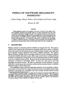
MARS (MAaintainable Real-time System) 11] is a fault-tolerant distributed realtime system architecture (see Figure 1). It is designed to serve as a basic system architecture for hard real-time applications. Main emphasis is put on a deterministic time behavior, even under anticipated peak load conditions, i.e., when all stimuli (events) occur with the speci�ed maximum frequencies. FTU 1
FTU 2
Node 1
q
Node 2
q q
q q
q
Node 5 FTU 3
q
Node 3
q q
q
Bus 1 Bus 2
Node 6
q
Node 4
q q
q q
q q
Node 7
Shadow
FTU 4
q q
q
Node 8
Shadow
Figure 1: MARS Cluster A MARS system consists of a set of clusters. They can be arbitrarily connected via cluster paths. Each cluster consists of a set of autonomous self-contained computers, called components. These components are loosely coupled by redundant synchronous real-time buses (MARS-buses). Each component consists of a single board computer and links to the real-time buses. Communication is realized solely by the exchange of broadcast messages, and access to the communication channel is controlled by a TDMA-strategy (time division multiple access). Components are assumed to be fail-silent. A \well-behaved" component produces either correct results or no results at all. As soon as it detects an error within itself, it turns itself o�. Extensive error detection mechanisms in hardware and software ensure a high self-checking coverage 13]. 5
To handle peak-load conditions, tasks are scheduled o�-line so that processor time is assigned to a task before run time. For this purpose an upper bound for each task's execution time is calculated in advance 15]. In most cases this calculated upper bound is signi�cantly larger than the real execution time. The remaining processor time is used for a second time-redundant execution of the task. This technique allows an e�cient detection of transient failures which can otherwise a�ect the application software. Fault-tolerance in MARS is based on the use of actively redundant components. Two actively redundant components form a fault tolerant unit (FTU). Since each component is fail-silent, full service can still be maintained after a component failure. However, a second failure in this FTU, before the failed component is \repaired" can lead to system crash. To handle this situation MARS introduces shadow components 13] which can be added to an FTU. Figure 1 shows a MARS cluster consisting of 4 FTUs. FTU 1 and FTU 2 consist of two actively redundant components while in FTU 3 and FTU 4 shadow components have been added. A shadow component operates in conjunction with the two actively redundant components. In contrast to the behavior of other components, a shadow component does not broadcast any messages on the MARS buses. In case of a failure of a working component, the shadow component takes over its operation. Since a shadow component receives and processes all incoming messages, it keeps its internal state equivalent to the actively redundant partner components. Therefore the switch from the failed component to the shadow component can be performed immediately after the component failure has been detected by the membership protocol 12]. Due to this service each working component has at time point tobserve a consistent knowledge about the operational states of the other components at time point tpast. The interval between tobserve and tpast is bounded above by two TDMA cycles.
3 Dependability models of MARS In this paper we investigate a MARS system consisting of one cluster consisting of n FTUs. FTUs within a cluster may have various kinds of dependencies. Extension to the case of multiple clusters can also be carried out. We analyze two di�erent MARS architectures. In the �rst variant each FTU consists of two actively redundant components. In the second case additional redundancy is added, decreasing the probability of spare exhaustion failures. Each FTU now consists of two actively redundant components and a shadow component.
6
3.1 Model Assumptions For modeling the MARS system the following assumptions will be made: � �
Faults occurring in one component are statistically independent of faults occurring in other components. In our models we include transient and permanent component faults. Each component's internal state can be decomposed into the h-state (history-state) and the i-state (initialization-state) 10]� accordingly, transient failures are distinguished as transient h-state and transient i-state failures. The h-state comprises all relevant information which has been accumulated in the sequence of computations since the initialization of the component. The i-state speci�es the contents of the read-only memory (i.e., program and permanent data). While the i-state of a component is �xed after initialization, the component's h-state changes during a computation. Therefore, three di�erent exponentially distributed failure types are considered for components:
{ Transient failures corrupting the h-state of a component with failure rate �h .
{ Transient failures corrupting the i-state of a component with failure rate �i .
{ Permanent failures occur with failure rate �p. �
These three di�erent types of component failures demand three di�erent repair actions:
{ A corrupted h-state only requires a new initialization of the component's history. The time to restore the component's h-state is exponentially distributed with rate �h. { If the i-state is corrupted, the component's i-state needs to be rebooted. This can be carried out periodically via a maintenance component with rate �i. { Repair of permanent failures is carried out with a constant repair rate �p. �
Due to the properties of the membership protocol the transient bus failure rate is subsumed in the failure rate of the components. Since two actively redundant buses are used, the e�ect of permanent bus failures is small enough to be omitted. 7
�
�
� �
The probability that the system successfully recovers from a component fault is called the coverage parameter c. Covered failures cause a component to be turned o�. With probability 1 ; c a failure is not covered. In this case we pessimistically assume that the system crashes. In this model, we assume that permanent failures have the same coverage parameter as transient failures. An operating maintenance component is required for restoring the i-state of a failed component. Since the maintenance component is actively redundant (with a shadow component), we assume that transient i-state failures can always be restored with rate �i. All repair activities subsequent to transient and permanent failures are assumed to be perfect. Shadow components do not send any messages on the buses, therefore we assume that a shadow component failure cannot lead to an FTU failure, which implies a perfect coverage for shadow component faults.
3.2 Model Parameters �
Based on our experiences and experiments with the existing MARS system we assume the following values for the failure rates:
{ Transient failures occur with rate �t = 1=3000 h;1. { Permanent failures occur with rate �p = 1=30000 h;1. �
Based on the relative sizes of the i-state and the h-state we choose �h = (4=5) � �t and �i = (1=5) � �t . Component failures are restored with the following rates:
{ For restoring a corrupted h-state, we assume �h = 120 h;1. { The reboot of i-state is carried out with rate �i = 12 h;1. { Permanent component failures are repaired with rate �p = 1=(7 � 24) h;1. �
We assume the following coverage value 13]: The hardware has a self-checking coverage of 99%. We further assume that the operating system can handle 90% of the operating system failures not covered by the hardware. Two-fold execution of application tasks �xes 99% of the remaining application software failures. Assuming 1=3 of the failures a�ect the operating system and 2=3 a�ect the application software, we achieve a coverage value of c = 0:99 + 0:01(1=3 � 0:9 + 2=3 � 0:99) = 0:9996 (see the tree diagram in Figure 2). 8
r
"b 0.99 "" bb 0.01 " b " b " b "detected by HW b : detected by HW ;@ ; @ @ 2=3 1=3 ; ; @ ; @ OS is a ected ; AS is a ected@ �A �A � A � A 0.9 � A 0.1 0.99 � A 0.01 � A � A � A � A � A � A r
r
r
r
detected by OS
r
r
: detected by OS
r
detected by AS
r
: detected by AS
Figure 2: Probability Tree
4 N-Versions of the MARS reliability model For modeling each of the two di�erent types of MARS systems (FTU without shadow component and FTU with shadow component) 3 versions of models have been developed. These models are solved using SHARPE or SPNP. In the following, we discuss the modeling techniques used for each of the 3 versions and explain the derived models. To keep the paper compact we restrict ourselves to presenting only the models for the MARS architecture using shadow components. Corresponding models for the architectural variant without shadow components can be easily derived.
4.1 Version 1: Hierarchical model In this version a largeness avoidance approach has been chosen. Each FTU is modeled as a continuous-time Markov chain (CTMC). Assuming that the FTUs are statistically independent, these CTMCs are hierarchically combined via a series block diagram to form a MARS cluster model. This version is evaluated using SHARPE. Following the chosen assumptions described in Section 3.1, for the architectural variant of an FTU with a shadow component, we derive the CTMC shown in Figure 3. Operational states are labelled wwjx or wjxx� x 2 fw� h� i� pg (w = working, h = transient h-state failure, i = transient i-state failure, and p = permanent failure). The number of w's to the left of the bar indicates the number of working components 9
�i
2c�i + �i
2(1 ; c)�g
�p
2c�p + �p
c� + � Figure 3: CTMC Model of an FTU 2with a Shadow Component h
h
2(1 ; c)�g
in the FTU. The letters to 2(1 the; right of the bar represent the states of the inactive c)� � components. F represents the FTU failure state. 2(1 ; c)� Assuming the same failure2rate for working components and shadow components, c� we derive a transition rate 2 � c � �y + �2yc�from state wwjw to state wwjy� y 2 fh� i� pg. � �components. The �rst term describes the covered� failure2c�rate of�the two working � 2The c� � 2 c� second term describes the shadow component failure rate. With rate 2 � (1 ; c ) � �g 2c� 2c� � c� � not covered and 2causes (where �2g� = �h + �i + �p ) a failure in state wwjw2is the FTU � 2c� from states failure. The failure transitions wwjy to wjyy are derived analogously. Component failures are recovered in parallel with rates �h � �i� and �p depending � � on the type of failure. � � g
h
g
i
i
i
i
h
h
p
p
p
p
h
i
p
g
h
p
h
i
�g
p
h
g
g
g
�g
4.2 Version 2: Stochastic Petri net model The hierarchical modeling approach provides a powerful yet e�cient technique for modeling large and complex systems. However, this approach assumes independence of the subsystems. This assumption precludes the modeling of global in�uences like shared maintenance personnel. In this version a stochastic Petri net (SPN) is used to compactly express the whole MARS cluster in one model. For ease of exposition, we �rst discuss the SPN model of a single FTU with shadow components (see Figure 4). We emphasize that the stochastic Petri net model description is only used for a convenient model speci�cation. This model is then internally transformed into a CTMC. The place working represents the working components. Initially, it contains two tokens. A third token is put in place shadow. The places h fail, i fail, and p fail represent a failed component, depending on the type of failure. A component failure occurs when transition fail h, fail i, or fail p �res. These �ring rates (�h � �i, and �p) are marking dependent. A failure can be covered (with probability c) or not covered (with probability 1 ; c), represented by the immediate transitions cov h, cov i, cov p, respectively n cov h, n cov i, n cov p. A covered component failure is repaired and the component becomes a shadow component when transition rep h, rep i, or rep p �res. The marking dependent �ring rates are �h� �i� and �p. The immediate transition sh to wo �res i� there are less 10
�� >�� }Z Z �� 6 � � Z
b
--2
shadow
�� 6
#�p rep p
#�i rep i
6
ZZ
#�h rep h
1:0
p
i
h
fail h
6
�� ��
@@ working � ZZ � � #� ZZ#� #� � � = fail i ? fail p Z~
sh to wo
? ? ? �� �� �� �� �� �� �� �� �� �� ��� ���� � � 6 6 6 � � �
p cov
cov p
i cov
6
cov i
h fail
h cov
6
cov h
c
�
6
1;c
i fail
p fail
c
c
�
1;c
�
1;c ?Q ? ? � n cov p n cov h Q n cov i � QQ ? �� Qs �+failed
�� ��
Figure 4: Stochastic Petri net model of an FTU then two tokens in place working. This transition is enabled by the inhibitor arc from place working. A MARS cluster consisting of n FTUs is modeled as an array with n such Petri (sub)nets. Firing stops if no token is in one of the places working in the array or one token is in one of the places failed in the array. In this case, to reduce the number of absorbing states in the underlying CTMC model, an immediate transition clear all �ushes all token from all places into a place called �nal. For the clarity of exposition, this transition is not shown in the �gure. The model developed here, provides a good basis for relaxing the assumption of FTUs' independence. Global in�uences like correlated failures, failure/repair dependencies, or stress factors could be easily incorporated by adding new transitions or modifying the �ring rates of existing transitions. Test runs have revealed (see Section 5) that the above described modeling approach is not directly appropriate for modeling a MARS system with shadow com11
ponents. Due to the massive use of redundancy, the state space grows tremendously. To reduce the state space, the use of state truncation is necessary. One attempt at getting the problem of state space explosion under control is the suppression of states with a low probability. Inspecting the failure and repair behavior of MARS components closely, one can realize that components spend only a small percentage of time in the state \transient failure". Due to the fault-tolerance mechanisms in MARS, 2 � n components can be concurrently in this state. However such operational system states with nearly 2 � n failed components caused through transient failures are extremely improbable. In our truncation approach we study the impact of truncating these states on the model size and the model result. For more details the reader is referred to Section 5.2.
4.3 Version 3: Folding of the stochastic Petri net Models as developed in Version 2 tend to become intractable for practical use. However, the models from Version 2 contain more information than is required for reliability analysis. If we assume that all FTUs are statistically identical then it is only necessary to keep track of how many FTUs are in each of their possible states. In particular, the identity of the state of each FTU is not important. This idea can be used to considerably reduce the overall state space. For this purpose the CTMC from Version 1 (see Figure 3) is interpreted as a stochastic Petri net. The states of the CTMC denote the places in the Petri net, while the state transitions of the CTMC are now interpreted as SPN transitions. Each token represents exactly one FTU, and a token in a particular place represents an FTU in this descriptive FTU state. For describing a MARS cluster with n FTUs, we just have to �ll in n tokens in place wwjw. The system fails (and all �ring stops) if at least one token reaches place F . Similar to the models from Version 2, these models provide a good basis for extensions, relaxing the assumption of FTUs' independence. As an example, we analyze the impact of a shared maintenance person. The model with shared repair is called Version 3.b (shared repair). It should be noted that this extension (3.b) does not change the number of states but only changes the transition rates in the underlying CTMC.
5 Discussion of the Results We analyze MARS clusters consisting from 1 up to 6 FTUs, assuming that all FTUs are needed to be operational. The main emphasis is placed on a comparison of the di�erent versions. Comparison criteria are the numerical results (MTTF), the 12
models' size (number of states and transitions), and the evaluation applicability (execution time). The next subsection concentrates on a comparison of the three basic versions. Subsection 5.2 studies the impact of truncation techniques applied on the model of Version 2. Finally, the assumption of FTU independence is relaxed in Subsection 5.3.
5.1 Comparison of the 3 basic Versions FTUs 1 2 3 4 5 6
Version 1 Hierarchical M. 2.42581590e+05 1.21362412e+05 8.09573191e+04 6.07542476e+04 4.86323846e+04 4.05511260e+04
Version 2 Stoch. Petri Net 2.42581580e+05 1.21363407e+05 8.09573157e+04 6.07542450e+04 4.86323826e+04 4.05511243e+04
Version 3 Folding 2.42581580e+05 1.21363407e+05 8.09573157e+04 6.07542450e+04 4.86323826e+04 4.05511243e+04
Table 1: MTTF in hours for FTUs without shadows FTUs 1 2 3 4 5 6
Version 1 Hierarchical M. 3.06489388e+06 1.53245962e+06 1.02164803e+06 7.66242256e+05 6.12998793e+05 5.10836484e+05
Version 2 Stoch. Petri Net 3.06487933e+06 1.53245215e+06 1.02164309e+06 ||||{ ||||{ ||||{
Version 3 Folding 3.06487933e+06 1.53245215e+06 1.02164309e+06 7.66238553e+05 6.12995833e+05 5.10834020e+05
Table 2: MTTF in hours for FTUs with shadows When comparing the output of the three versions we start with the MTTF. Since di�erent techniques have been used for generating the models, this comparison supports a model validation. At the same time, these models have been evaluated by di�erent tools. These two aspects { di�erent modeling techniques and di�erent tools { increase the modeler's con�dence in the numerical model results. This comparison also allows a validation of the model solution algorithms of SHARPE and SPNP. Tables 1 and 2 show the MTTF in hours for the three basic versions. A comparison of the results shows that Version 2 and 3 (both evaluated with the SPNP 13
package) produce exactly the same results. Version 1 (solved using SHARPE) computes a slightly di�erent result� the di�erence being negligible. For the MARS architecture with shadow components, Version 2 does not produce any results for clusters with 4 or more FTUs. To further investigate this fact, let us have a closer look to the Tables 3 { 6. FTUs 1 2 3 4 5 6
Version 1 Version 2 Version 3 Hierarchical M. Stoch. Petri Net Folding states trans. states trans. states trans. 5 10 5 10 5 10 5 10 17 64 11 34 5 10 65 352 21 80 5 10 257 1792 36 155 5 10 1025 8704 57 266 5 10 4097 40960 85 420
Table 3: CTMC Sizes for FTUs without shadows FTUs 1 2 3 4 5 6
Version 1 Version 2 Version 3 Hierarchical M. Stoch. Petri Net Folding 0.1 0.3 0.3 0.1 0.7 0.4 0.1 2.9 0.5 0.1 21.7 0.7 0.1 223.2 0.9 0.1 2871.6 1.2
Table 4: Execution Time in seconds for FTUs without shadows Tables 3 and 5 show the CTMC sizes in terms of number of states and transitions. Table 4 and 6 list the execution time in seconds on a DEC-station 3100 con�gured with 16 MByte main memory and 128MBytes swap space. The execution time values serve only as trends for the computational e�ort and are not intended as machine or evaluation program benchmark. It should be noted that the elapsed time could be signi�cantly larger than the execution time due to the swap activities. The data show that the use of shadow components in Version 2 soon results in a mathematically intractable model, caused through the state explosion of the CTMC. One can see that the folding technique, applied in Version 3, is a promising approach in handling the model largeness. 14
FTUs 1 2 3 4 5 6
Version 1 Version 2 Version 3 Hierarchical M. Stoch. Petri Net Folding states trans. states trans. states trans. 11 34 11 34 11 34 11 34 101 580 56 295 11 34 1001 8200 221 1540 11 34 ||{ 716 5995 11 34 |{ |- 2003 19162 11 34 |{ |- 5006 53053
Table 5: CTMC Sizes for FTUs with shadows FTUs 1 2 3 4 5 6
Version 1 Version 2 Version 3 Hierarchical M. Stoch. Petri Net Folding 0.2 1.5 1.3 0.2 13.9 6.4 0.2 317.9 30.8 0.2 |{ 152.9 0.2 |{ 538.5 0.2 |{ 1551.5
Table 6: Execution Time in seconds for FTUs with shadows Completely di�erent is the situation in Version 1. Due to the \divide and conquer" principle, the hierarchical modeling approach is most rewarding in dealing with the model complexity. Since each FTU is analyzed separately and then hierarchically combined via a series block diagram. An additional FTU in a MARS cluster does not a�ect the model size and complexity. However, this approach implies FTUs' independence, an assumption which can be relaxed in Versions 2 and 3 (see Subsection 5.3).
5.2 State Truncation State explosion of the CTMC model makes a practical evaluation of models from Version 2 with 4 or more FTUs with shadow components infeasible. However, many of these states are only reached with extremely low probability. A suppression of these states can cause a signi�cant reduction of the model states without signi�cantly a�ecting the accuracy of the results. In this subsection we illustrate the impact of truncation techniques and provide a 15
comparison of di�erent truncation levels with respect to the MTTF, the model size, and the execution time. To study the impact of truncation on the MARS cluster, we de�ne truncation levels. Truncation level 0 means no truncation at all. Since a MARS cluster with n FTUs can tolerate 2 � n \transient failed components", at truncation level 1 states representing a system with 2 � n \transient failed components" are considered to be absorbing states. This system can therefore tolerate 2 � n ; 1 transient faults concurrently. Similarly at truncation level i the system can tolerate 2 � n ; i transient faults concurrently. In the �rst experiment, we consider a system with 3 FTUs, with truncation levels 5 to 0. Table 7 illustrates the rapid decrease of the model size and its execution time. Further note that below truncation level 4, the resulting MTTF remains essentially the same. Trunc. Model size Execution MTTF level states trans. Time 5 136 855 23.1 8.59848920e+05 4 361 2568 83.5 1.02163808e+06 3 641 4936 172.6 1.02164308e+06 2 866 6949 256.8 1.02164309e+06 1 974 7957 313.9 1.02164309e+06 0 1001 8200 323.3 1.02164309e+06
Table 7: Truncation for a MARS cluster with 3 FTUs The slightly larger execution time for truncation level 0 in this version compared with Version 2 with 3 FTU and no truncation at all is caused by the more complex description of the enabling function for �ushing all tokens if all �ring stops. In the second experiment, we analyze a MARS cluster with 4 FTUs. This model is evaluated with truncation levels 7 to 4. We note that a MARS system model Version 2 with 4 FTUs cannot be solved without state truncation. However, it can be solved to provide su�ciently accurate results using truncation.
5.3 Global In�uences Models developed in Version 3 provide a good basis for relaxing the assumption of FTU's independence. In the next experiment we assume that there is only one shared repair person for �xing permanent component failures. Since this model modi�cation does not change the model size, we only list the MTTF here. In Table 9 and 10 we illustrate the impact of the shared repair person on system's 16
Trunc. Model size Execution MTTF level states trans. Time 7 514 3969 144.6 6.08702785e+05 6 1702 14805 835.9 7.66231039e+05 5 3766 35605 2718.9 7.66238553e+05 4 6236 62315 8356.1 7.66238553e+05
Table 8: Truncation for a MARS cluster with 4 FTUs FTUs 1 2 3 4 5 6
Version 3 Ind. Repair 2.42581580e+05 1.21363407e+05 8.09573157e+04 6.07542450e+04 4.86323826e+04 4.05511243e+04
Version 3.b Shared Repair 2.42581580e+05 1.20396946e+05 7.96728606e+04 5.93139935e+04 4.71012799e+04 3.89616962e+04
Table 9: Comparison of the MTTFs for FTUs without shadows MTTF. It is evident that the in�uence of the shared repair person increases, due to the growing down-time intervals of permanently failed components, with the number of components. For a MARS cluster with 6 FTUs without shadow components the shared repair person's impact is 4%. Using FTUs with shadow components it reaches 10%. FTUs 1 2 3 4 5 6
Version 3 Ind. Repair 3.06487933e+06 1.53245215e+06 1.02164309e+06 7.66238553e+05 6.12995833e+05 5.10834020e+05
Version 3.b Shared Repair 2.79959899e+06 1.39982852e+06 9.33238360e+05 6.99943277e+05 5.59966226e+05 4.66648191e+05
Table 10: Comparison of the MTTFs for FTUs with shadows 17
6 Conclusion We have analyzed the MARS architecture using di�erent modeling techniques and two di�erent evaluation tools. The modeling techniques have been compared in terms of their numerical results (MTTF), their model size (number of states and transitions), and their evaluation applicability (execution time). The numerical results have revealed that due to the massive use of redundancy in MARS, brute force methods such as the formulation of the MARS cluster in one stochastic Petri Net, soon result in mathematically intractable models. Using advanced modeling techniques such as folding of Petri Nets, suppression of states with low probability via state truncation, or hierarchical modeling, the problem class can be solved with state-of-the-art evaluation tools in reasonable time.
References �1] R. Butler. An Abstract Language for Specifying Markov Reliability Models. IEEE Transactions on Reliability, 35(5):595{601, Dec. 1986. �2] J. A. Carrasco and J. Figueras. METFAC: Design and Implementation of a Software Tool for Modeling and Evaluation of Complex Fault-Tolerant Computing Systems. In Proc. 16th Int. Symposium on Fault-Tolerant Computing, pages 424{429, Vienna, Austria, July 1986. �3] G. Ciardo, J. Muppala, and K. Trivedi. SPNP: Stochastic Petri Net Package. In Proc. 3th Int. Workshop on Petri Nets and Performance Models, pages 142{151, Kyoto, Japan, Dec. 1989. �4] A. Costes, J. E. Doucet, C. Landrault, and J. C. Laprie. SURF: A Program for Dependability Evaluation of Complex Fault-Tolerating Computing Systems. In Proc. 11th Int. Symposium on Fault-Tolerant Computing, pages 72{78, Portland, Maine, June 1981. �5] J. B. Dugan, K. S. Trivedi, M. K. Smotherman, and R. M. Geist. The Hybrid Automated Reliability Predictor. AIAA Journal of Guidance, Control and Dynamics, 9(3):319{331, June 1986. �6] J. B. Dugan and K. S. Trivedi. Coverage Modeling for Dependability Analysis of FaultTolerant System. IEEE Transactions on Computers, 38(6):775{787, June 1989. �7] R. Geist and K. Trivedi. Reliability Estimation of Fault Tolerant Systems: Tools and Techniques. IEEE Computer, 23(7):52{61, July 1990. �8] A. Goyal, W. C. Carter, E. de Souza e Silva, S. S. Lavenberg, and K. S. Trivedi. The System Availability Estimator. In Proc. 16th Int. Symposium on Fault-Tolerant Computing, pages 84{89, Vienna, Austria, July 1986.
18
�9] A. M. Johnson and M. Malek. Survey of Software Tools for Evaluating Reliability, Availability and Serviceability. ACM Computing Surveys, 20(4):227{269, Dec. 1988. �10] H. Kopetz. The Failure Fault (FF) Model. In Proc. 12th Int. Symposium on FaultTolerant Computing, pages 14{17, Santa Monica, California, June 1982. �11] H. Kopetz, A. Damm, Ch. Koza, M. Mulazzani, W. Schwabl, Ch. Senft, and R. Zainlinger. Distributed Fault-Tolerant Real-Time Systems: The MARS Approach. IEEE Micro, 9(1):25{40, Feb. 1989. �12] H. Kopetz, G. Gr�unsteidl, and J. Reisinger. Fault-Tolerant Membership Service in a Synchronous Distributed Real-Time System. In 1st Int. Working Conference on Dependable Computing for Critical Applications, pages 167{174, Santa Barbara, CA, USA, Aug. 1989. �13] H. Kopetz, H. Kantz, G. Gr�unsteidl, P. Puschner, and J. Reisinger. Tolerating Transient Faults in MARS. In Proc. 20th Int. Symposium on Fault-Tolerant Computing, pages 466{473, Newcastle upon Tyne, UK, June 1990. �14] M. Mulazzani and K. S. Trivedi. Dependability Prediction: Comparison of Tools and Techniques. In IFAC Proceedings SAFECOMP 86, pages 171{178, Sarlat, France, Oct. 1986. �15] P. Puschner and Ch. Koza. Calculating the Maximum Execution Time of Real-Time Programs. Real-Time Systems, 1(2):159{176, Sep. 1989. �16] R. A. Sahner and K. S. Trivedi. Reliability Modeling using SHARPE. IEEE Transactions on Reliability, 36(2):186{193, June 1987. �17] W. Sanders and J. Meyer. METASAN: A Performability Evaluation Tool based on Stochastic Activity Networks. In ACM-IEEE 1986 Fall Joint Computer Conference, Nov. 1986. �18] L. Tomek and K. Trivedi. Fixed Point Iteration in Availability Modeling. In 5th Int. Conference on Fault-Tolerant Computing Systems, Test, Diagnosis and FaultTreatment, N�urnberg, Germany, Sep. 1991.
19