IEEE TRANSACTIONS ON MULTI-SCALE COMPUTING SYSTEMS, VOL. XX, NO. X, FEBRUARY 2018
1
Design Methodology for Responsive and Robust MIMO Control of Heterogeneous Multicores Tiago Muck, Student Member, IEEE, Bryan Donyanavard, Student Member, IEEE, ¨ Kasra Moazzemi, Student Member, IEEE, Amir M. Rahmani, Senior Member, IEEE, Axel Jantsch, Member, IEEE, and Nikil Dutt, Fellow, IEEE Abstract—Heterogeneous multicore processors (HMPs) are commonly deployed to meet the performance and power requirements of emerging workloads. HMPs demand adaptive and coordinated resource management techniques to control such complex systems. While Multiple-Input-Multiple-Output (MIMO) control theory has been applied to adaptively coordinate resources for single-core processors, the coordinated management of HMPs poses significant additional challenges for achieving robustness and responsiveness, due to the unmanageable complexity of modeling the system dynamics. This paper presents, for the first time, a methodology to design robust MIMO controllers with rapid response and formal guarantees for coordinated management of HMPs. Our approach addresses the challenges of: (1) system decomposition and identification; (2) selection of suitable sensor and actuator granularity; and (3) appropriate system modeling to make the system identifiable as well as controllable. We demonstrate the practical applicability of our approach on an ARM big.LITTLE HMP platform running Linux, and demonstrate the efficiency and robustness of our method by designing MIMO-based resource managers. Index Terms—Heterogeneous multiprocessors, MIMO, Control theory, System modeling, Resource management
F
1
I NTRODUCTION
M
multicores must support diverse workloads that exhibit varying resource demands, sometimes with conflicting constraints. Workload characteristics (e.g., memory-bound, compute-bound) may vary across applications executing concurrently, posing significant challenges for homogeneous architectures [1], [2]. Emerging heterogeneous multicore processors (HMPs) deploy heterogeneous compute elements on a single chip, allowing tradeoffs between objectives such as maximizing performance and minimizing power consumption. For instance, ARM’s big.LITTLE architecture [3] deploys cores with more cache and compute capacity (big), alongside low power and low performance cores (LITTLE). These HMPs require sophisticated and adaptive resource management due to the presence of multiple architecturally differentiated cores supporting diverse workloads. Contemporary approaches utilize heuristics to optimize a single objective in order to manage resources at runtime [4], [5], [6], [7]. However, realistic scenarios demand simultaneous management of multiple objectives (e.g., best performance within a thermal cap), resulting in the challenge of tuning a large configuration space of reconfiguration parameters. Ad-hoc approaches are not robust: coordinating and prioritizing actuators is not straightforward and often requires complex algorithms. Additionally, with ad-hoc approaches, there are no guarantees that the system will avoid an unstable state when workloads are unpredictable. Control theoretic approaches for resource management (e.g., [8], [9], [10], [11], [12], [13], [14]) provide formal guarantees for achieving robustness and stability, particularly in the presence of workload variability. MultipleInput-Multiple-Output (MIMO) control theory is effective • • •
ODERN
Tiago Muck, ¨ Bryan Donyanavard, Kasra Moazzemi, Amir M.Rahmani, and Nikil Dutt are with the University of California, Irvine, USA. E-mail: {tmuck, bdonyana, moazzemi, amirr1, dutt}@uci.edu Amir M. Rahmani and Axel Jantsch are with the TU Wien, Vienna, Austria. E-mail:
[email protected] This work was partially supported by NSF grant CCF-1704859, the Marie Curie Actions of the EU’s H2020 Programme, and CAPES (CSF program)
for coordinating management of multiple goals in unicore processors [15]. However, MIMO control for HMPs poses additional challenges and complexity in system modeling, development of robust controllers, and guaranteeing stability in the face of dynamic and unpredictable system behavior. We demonstrate that directly applying a classic MIMO approach ([15]) leads to controller designs that either lack robustness (i.e, are highly susceptible to instability) or manifest poor responsiveness (i.e., the speed with which a new target objective can be met), mainly due to unmanageable system identification complexity. An appropriate dynamic system modeling (i.e., identification) and decomposition strategy is needed to account for considerations such as size of the system, heterogeneity of cores, and scope of the actuators and sensors in HMPs. Once the system dynamics are properly modeled, several off-the-shelf robust controller design techniques are available for building a stable and responsive resource manager. Our work presents, for the first time, a methodology to design robust and responsive MIMO controllers for coordinated management of HMPs with formal guarantees. The main contributions of this paper are: • System modeling guidelines for formulating robust and responsive MIMO control of complex HMPs. This includes a set of properties for the system to be controllable, efficient, and robust. We enable tuning of the controller by simplifying the identification of dynamic systems. Demonstration of the practical efficacy of our ap• proach on an 8-core ARM big.Little development board. We coordinate the platform’s power and performance objectives while experiencing disturbance caused by background tasks and task migration.
2
BACKGROUND
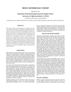
MIMO control for coordinated resource management [16], [15] has generalized management of multiple controllers or objectives for a single-core processor. Consider the MIMO controller in Figure 1 that controls a system with two control
IEEE TRANSACTIONS ON MULTI-SCALE COMPUTING SYSTEMS, VOL. XX, NO. X, FEBRUARY 2018
2
Fig. 1: Basic 2 × 2 MIMO. inputs and two interdependent measured outputs. The MIMO is implemented using a Linear Quadratic Gaussian (LQG) controller [17]:
x(t + 1) = A × x(t) + B × u(t) y(t) = C × x(t) + D × u(t)
(1) (2)
where x,y , and u are vectors representing the system state, the measured outputs, and the control inputs, respectively. Coefficient matrices A, B , C , and D capture the system behavior, and their values are obtained through system identification. Matrix sizes are determined by both the number of inputs and outputs of the controller as well as the order of the controller. The MIMO design process consists of: 1) defining the system to be controlled by specifying inputs and outputs; 2) using experimental data to identify the system model; 3) designing and tuning the controller based on the system model; and 4) analyzing and validating the robustness and stability of the designed controller. In this paper we focus mostly on steps (1) and (2). Once the controlled system is defined, the first step in system identification is generating test waveforms from training applications in order to create a system model. For complex systems it is more common and feasible to use statistical or black-box methods based on System Identification Theory [18] for isolating the deterministic and stochastic components of the system to build the model. Given an order, the model estimation generates the A, B , C , and D matrices (Equation 1, 2). The order dictates the dimension of the model (i.e., size of the state space), which is typically a trade-off between accuracy and complexity. Once the model is created, it is cross-validated using a different data set and the model uncertainty is assessed using Robust Stability Analysis[18]. The higher the uncertainty guardband, the more robust is the model and therefore the generated controller. Picking actuators and measurement metrics that result in behavior that can be estimated linearly is one of the most important aspects of designing a stable controller [19]. Reducing model uncertainty is crucial for the stability of a controller: perturbations due to model uncertainty can destabilize a system; if system identification is completed successfully, the remaining steps in controller design are trivial. In the following sections, we describe a set of properties to use when defining systems or subsystems for MIMO design, and demonstrate why the controlled system should exhibit these properties for the controller to identify controllable, efficient, and robust models for complex systems.
3
C ONTROLLABLE HMP M ODELS FOR MIMO D E -
SIGN
We now illustrate the challenges faced in designing robust and efficient MIMO control for HMP systems from the perspectives of: (1) determining the optimal input/output MIMO configuration; (2) establishing uniformity for system identification; (3) managing the scope of sensors and actuators for model fitting; and (4) minimzing the model size to handle complexity. We use the case study shown in Figure 2
Fig. 2: Example system overview. to highlight these challenges and motivate the need for an overall methodology for MIMO design that establishes the desired guarantees. Figure 2 shows the ODROID 8-core big.LITTLE Exynos 5422 HMP platform executing a set of representative applications on top of Linux or Android, thereby emulating the background noise in real platforms. Consider the systemlevel perspective of this HMP as depicted in Figure 3(a). This abstraction shows the sensors and actuators available for the 8-core HMP. Suppose we are interested in controlling the system throughput in terms of instructions per second (IPS) while monitoring the power by using operating frequency and injected idle cycles. The design of a LQG MIMO controller (Equation 1, 2) is a well understood process. The main challenge is defining a system to identify and control this processor. There are several pitfalls to address before designing the controller. For example, let us define a MIMO using all frequency and idle cycle inputs, and IPS and power outputs. First, the resulting controller would be of size 10×10. Not only would the system be challenging to identify, the resulting controller would be sluggish and complex to execute at runtime. Second, the selected mix of control inputs have varied effects on measured outputs: frequency uniformly affects an entire cluster and its outputs, while idle cycle injection affects per-core IPS and total cluster power. Note that black-box identification techniques have no internal information about subsystems, and simply try to relate the changes of any input to an impact on any output. If a sensor only partially exercises the system and, consequently, a subset of outputs, the outputs not involved are considered unfavorably in the model. Furthermore, identifying a statespace MIMO system needs training sets varying all inputs simultaneously (e.g., a set of out-of-phase staircase signals for the control inputs [20]). If the inputs and output are not uniformly correlated, isolation of the deterministic and stochastic aspects of the system may be inaccurate. Third, heterogeneity of core types can make the black-box system identification challenging (i.e., inaccurate or complex) if an output is correlated to more than one core type (e.g., power capping using a chip-level power sensor in HMPs). Subsystem asymmetry complicates system identification and increases model uncertainty. Note that these are conservative assumptions for system complexity. Platform complexity will continue to increase in the future (e.g., Mediatek’s 10-core 3-cluster HMP SoC with two 2.5GHz ARM A72, four 2.0GHz high-performance A53, and four 1.4GHz energy-efficient A53 cores), further exacerbating these challenges. In this context, the properties we are concerned with are controllability, robustness, and efficiency. These properties are critical to ensure that the closed-loop system is stable (does not show large oscillations) and robust to disturbance, while rapidly converging to the desired state.
IEEE TRANSACTIONS ON MULTI-SCALE COMPUTING SYSTEMS, VOL. XX, NO. X, FEBRUARY 2018
3 Measured and simulated model Power
Measured and simulated model IPS
100
10
0
0
-100
Time 100
200
300
400
-10 500 Time 100
Simulated model
200
300
400
500
Measured output
Fig. 4: (Left) Real vs. modeled IPS output of an 8×8 system. (Right) Real vs. modeled power output of an 8×8 system.
In the following, we demonstrate the need for an overall control design methodology to satisfy these properties. Guidelines presented highlight the challenges in the system identification process and provide insight about coordinated strategies to ensure the properties. 3.1
Model Size
The number of control inputs and measured outputs are critical for determining the system to be controlled by an individual MIMO. There are formal requirements in MIMO design on number of inputs and outputs (e.g., #inputs ≥ #outputs), and these values determine the size of the controller and its responsiveness. Systems with large numbers of inputs and outputs are more difficult to identify and provide smaller robustness confidence intervals. If identifiable, such a system will generate a sluggish controller that requires heavy computations at every epoch due to the size of state-space matrices. Figure 3(b) depicts this challenge, where the latency of the controller (to respond to changes in environment) can be decreased by breaking down the system into smaller subsystems with manageable size. In order to demonstrate the issues with system identification of MIMO controllers with a large number of control inputs and measured outputs, we simulate an 8×8 system similar to [16]. Using the gem5 architectural simulator [21] we construct a homogeneous system comprised of four computing cores. For control inputs to the system we use percore core clock frequency and cache size. Measured outputs are per-core power and IPS. The simulation is designed to isolate the size issue from other pitfalls discussed in this section. Figure 4 compares the real output and modeled output for the same set of inputs. The inaccuracy of the modeled IPS and power show the difficulty in identifying a system model for a large system. 3.2
System Uniformity
Systems that are composed of uniform subsystems can be identified more easily than those with varying subsystems (e.g., Figure 3(c)). One of the main challenges in identifying HMPs compared to CMPs or single-core systems is the heterogeneity in compute units. In addition to having nonuniform
3.3
Scope of Controllability
Selecting actuators and measurement metrics that result in stable, ideally linear, relations is one of the most challenging and important tasks when designing a controllable MIMO. Some actuators have different granularity and operate in various scopes, such as task-level, core-level, system-wide,
Autocorrelation
Fig. 3: System-level views: (a) Exynos 5422 8-core HMP with sensors and actuators; (b) Large number of sensors and actuators; (c) Nonuniform subsystems; (d) Discrete scope of sensor and actuators.
characteristics, heterogeneous systems can have different actuation configurations for various elements, which requires proper care in system identification. One example is a larger range of operating frequencies for high-performance cores compared to energy-efficient cores. To mitigate the effects of this heterogeneity, the system can be decomposed into subsystems that control uniform elements. In order to compare the accuracy of system identification in uniform and nonuniform systems, Figure 5 shows residual auto-correlation for three sets of MIMO models in our case study. Residual is the stochastic component (e.g., disturbance, noise) of the system output, which is not supposed to be included in the model. If there is no correlation between the residual and itself or any inputs, the model is good. In this context, there are two important properties in the residual function that need to be ensured: 1) the residual should not affect the confidence levels (i.e., the probability with which the true output will fall into the confidence interval range[22]); 2) the spectrum of samples should not show any peaks, falls, or patterns (except around zero). In other words, the residual correlation for different samples (Fig. 5 x-axis) should look like pure noise. If a model violates either of these two properties, the controller generated from this model will likely fail the robustness analysis. Two of the models in Figure 5 are designed to control a dual-core uniform system (either two Cortex-A15 cores or two Cortex-A7 cores), and the third model represents a heterogeneous system (CortexA15 and A7). The result of auto-correlation shows that for the same set of experiments, uniform systems maintain a residual mean around zero while the nonuniform case operate outside confidence intervals. This property will result in high uncertainty and can easily make the corresponding controller unstable. Benefiting from architectural insight about the uniformity of underlying subsystems can improve the quality of system model.
0.4 A7-A7
A15-A7
A15-A15
Confidence interval
0.2 0 -0.2 -20
-15
-10
-5
0
5
10
15
20
Samples
Fig. 5: Residual comparison between uniform and nonuniform subsystem modeling. The horizontal scale is the number of lags, which is the time difference (in Samples) between estimated correlation.
Measured and simulated model IPS
4
5
2
0
0
-5 -2
-10 0
20
Time
0.2
Autocorrelation
4
6
Measured and simulated model power
4
Normalized IPS
10
40 60 0 20 Time Simulated model Measured outputs
40
60
2 0 -2 Order 4 Order 3 Order 2 ref
-4 -6 -8 0
0
-0.2 -20
10
20
30
40
50
60
Time Confidence Interval -15
-10
-5
0
Samples
5
10
Model 15
20
Fig. 6: Top: Real vs. modeled IPS and Power measured outputs, normalized around the mean. Bottom: Confidence interval violations of residual function in a MIMO controller with inconsistent actuator scope. etc. Choosing actuators with the same scope results in a more accurate system system model, and robust controller. The top plots in Figure 6 show real and modeled output for IPS and power of the ODROID platform. The model is for a system that controls clock frequency of each cluster (clusterlevel actuator), and number of active cores for the whole platform (system-level actuator), in order to track system power and IPS. The model for this system attempts to mimic power behavior but fails to show an acceptable simulated output behavior for IPS references. In the lower plot of Figure 6 we observe that this model many peaks that break the boundaries of the 99% confidence intervals, violating both desired residual properties. In the next section, we show how well a model can fit the measured data if a more careful combination of subsystems and sensors/actuators is selected. 3.4 Model Minimality Selecting the suitable system order when defining a system to identify is one of the important challenges in designing a controllable system. The model order directly affects the complexity of the resulting controller implementation. The order will determine the accuracy, confidence in modeling, and additional computation for decision making. Higher order models generally1 provide higher accuracy, but the resulting controllers require more computation for each control decision, and respond sluggishly to rapid changes. Therefore, both architectural insight and complexity analysis are needed to choose the proper model order. For system identification of MIMO controllers, Matlab provides recommendations based on a singularity function which can give designers insight about the model behavior. The case study system in this section is constructed using a big cluster with four CortexA15 cores. This model has two inputs (clock frequency and number of active cores) to control two measured outputs (IPS and Power). Figure 7 shows an example of an output (IPS) modeled using three different orders. This system has desirable size, sensors/actuators, and uniformity, which all together result in a suitable system identification. The last design decision is the order of the model. In most cases, models with higher order mimic the true IPS with more precision. However, it should be noted that order-two has 89.99%, order-three 90.53% and order-four has 90.58% fitting association. As we go to even higher orders, the improvement on accuracy 1. Over-fitting is possible.
Fig. 7: Modeled vs. true IPS (normalized to mean) of CortexA15 four-core system for different model orders.
diminishes. It is the designer’s responsibility to select the proper order for the model that provides good enough accuracy while maintaining controller efficiency; however, the rule of thumb is that a fitting value of larger than 80% is often good enough [20]. We also refer to the Matlab system identification recommendation for a set of various MIMOs. First, the 10×10 MIMO described in Section 3.1 has the recommended order 20, which was the maximum order allowed by the tool. On the other hand, 4×2 and 4×4 MIMOs with various actuator scope had recommended orders between 3 to 5. This shows that not only are large systems penalized due to size of state space matrices, but are also required to store many prior measurements and actuations to capture the dynamics of the system. Figure 8 shows a complementary analysis in selecting model order for the same case study. In this figure, the autocorrelation function for the residuals for three different orders of our big cluster system are computed and illustrated. The confidence interval for these functions is shown as dashed lines. For an acceptable model, the correlation curves should lie between these lines and not show any peaks, falls, or patterns. As we can observe, the first-order model has many confidence violations, which indicates the controller designed from this model would not be robust. While the third-order model shows improved behaviour, the fifth-order model exhibits a peak around 9 and -9 due to over-fitting. This indicates that in some corner cases the controller generated from this model may become unstable. The ability to avoid unstable states in our closed-loop system is one of the advantages of our proposed guidelines. 3.5
Mixture of issues
To demonstrate the aggregated effect of issues mentioned in this section on a real system, we use a 10×10 model similar to Figure 3(a) with cluster frequency and core idle cycles as control inputs, and cluster power and core IPS as measured outputs. Figure 9 shows the fit and residual for the system identification. The model shows high error between real and modeled data, which indicates that it cannot capture
Order 1
Order 3
Order 5
99% Confidence interval
0.1
Autocorrelation
Normalized output
IEEE TRANSACTIONS ON MULTI-SCALE COMPUTING SYSTEMS, VOL. XX, NO. X, FEBRUARY 2018
0.05 0 -0.05 -0.1 -20
-15
-10
-5
0
5
10
15
20
Samples
Fig. 8: Residual for Cortex-A15 four-core systems of different orders.
IEEE TRANSACTIONS ON MULTI-SCALE COMPUTING SYSTEMS, VOL. XX, NO. X, FEBRUARY 2018 Big core power model
Normalized output
1
Little core power model 0.5
Specifications
Objectives
2
0.5 0 0
0
20 Time 40
60
-1 20 Time 40
0
Simulated model output
60
Check size 20 Time 40
0
R2>80
0 Confidence interval
-10
-5
0
heterogeneity
Measured output
0.5
-15
sensors/actuators
60
1
-0.5 -20
Compute units type
System decomposition
-0.5 -0.5
System structure
System
Sensor/ Actuator list
1 0
-1
Autocorrelation
Sample core IPS model
5
5
10
System identification
No residual peaks
confidence interval
Min order
Sample model
15
Controller design
20
Samples
Off-the-shelf controllers and well established controller design techniques
Fig. 9: Top: Fit of the simulated model associated with three of the ten outputs, normalized around the mean. Bottom: Residual function of one of the outputs in 10×10 MIMO w.r.t. 99% confidence intervals.
Robustness analysis Check uncertainty
Robustness
Objective verification
Deploy
the dynamics of the system, and may result in instability and high steady state error. More importantly, this system requires an order of 20 (due to its singularity value [18]) for identification which means the controller should consider inputs (u(t)) and output (y(t)) for many previous iterations in its state matrix. This would impose a large memory requirement and computational overhead in the controller which will result in a slow settling time. The bottom plot in Figure 9 shows auto-correlation of residuals for one of the outputs and the correlated confidence intervals. In this example, though the autocorrelation of the residual exhibits no patterns, it fails to fall within the 99% confidence interval range, thus showing the importance of selecting proper size, uniformity, scope, and order in MIMO design process.
4
C ONTROL D ESIGN M ETHODOLOGY
We now present our overall MIMO control design methodology for HMPs, including guidelines for ensuring a more robust and stable closed-loop system, as outlined in Figure 10. Specifications: The designer must begin by defining or specifying a) the management objectives of the system (e.g., energy efficiency, maximum throughput, power capping, etc.), (b) the computer system structure (e.g., VF islands, nodes, processors), (c) compute unit description (e.g., type and number of cores and accelerators), and (d) list of sensors/actuators and their scope for the computer system. These specifications are necessary for system decomposition and identification. System decomposition: This step consists of finding all the valid combinations of specifications that compose controllable subsystems for managing the desired objective(s). This process eliminates potential systems with an uncontrollable number of inputs and outputs or subsystems with insufficient actuators. It is important to ensure that each measurable output of a subsystem is necessary and appropriate for achieving the overall objective(s). For example, selecting the entire processor as the system model to identify in order to manage a single core’s temperature is a poor choice that will result in an inefficient controller. In the case that a system can be divided into uniform or nonuniform subsystems, uniform decomposition is highly preferred. System identification: This is the critical step in designing MIMO controllers for HMPs. Here, all candidates found during system decomposition are modeled and evaluated in terms of their residual behaviour, and their associated
Fig. 10: MIMO design methodology for HMPs fit to measured data and model order. Black-box system identification is performed to find system models exhibiting an acceptable fitting value. Based on a rule of thumb in control theory, if the coefficient of determination, also known as R2 , is greater or equal than 80%, the model will be acceptable [20]. In case there are multiple valid candidates that satisfy these requirements, the model with minimum order will be selected for controller design. On the other hand, if there is no model found having all the recommended properties, confidence intervals can be expanded (i.e., relaxed) to include at least one system model. These boundaries are used in the last step for robustness analysis. Controller design: Given that our guidelines for system decomposition are followed and the resulting system is identifiable, the design of the controller itself (i.e., finding the coefficient matrices for Eqs. 1 and 2) is a well-established field where off-the-shelf tools can be used. Design of MIMO controllers for computing systems is extensively explained in [20] and [15]. Robustness analysis: In this final step, we check if the controller can tolerate disturbance based on a defined uncertainty level while maintaining the specified confidence (i.e., remaining stable). In addition, we ensure that the chosen controller can meet the design objectives. At this stage, all unaccounted elements, modeling limitations, and environmental effects are estimated as model uncertainties. The designer must ensure the controller is stable for all the uncertainties. For example, we can confirm our MIMO controller is robust enough to reject the disturbance from background tasks and is able to react efficiently in case of task migration from one cluster to the other. If the designed controller cannot meet the requirements of the closed-loop system, we return to system identification and select a higher order model for a new controller design iteration.
5
R ESULTS
Our goal is to evaluate two distinct MIMO configurations, one which satisfies the conditions defined in Section 4, and one which does not, in terms of their ability to track performance and power goals on an HMP. Our evaluation is done using the ODROID-XU3 platform with an Exynos 5422 HMP (Table 1) running Ubuntu Linux. This platform has four ARM A15 cores and four ARM A7 cores divided into two clusters. DVFS is applied at the cluster-level, but cores
IEEE TRANSACTIONS ON MULTI-SCALE COMPUTING SYSTEMS, VOL. XX, NO. X, FEBRUARY 2018
Parameter (Core type) Issue width L1$I/$D size (KB) L2 size (KB)1 Max VF Min VF 1
big (Cortex A15)
LITTLE (Cortex A7)
4 (OoO) 32/32 2048 2.0GHz/1.2V 1.2GHz/1.0V
2 (Inorder) 32/32 512 1.4GHz/1.2V 1.0GHz/1.1V
IPS(∗109 ) ref1
Per cluster shared L2 caches
can be clock-gated individually. Memory is shared across all cores, so application threads can transparently execute on any core. We consider a typical mobile scenario in which one or more multithreaded applications execute concurrently across the HMP. 5.1 Experimental Setup Controller Configurations: We design two control-based resource managers. 1) Two individual 2×2 MIMOs, one for each cluster. Each controller tracks an IPS and power reference for its cluster. The controlled inputs are the cluster clock frequency and the number of active cores in the cluster. 2) A single system-wide 4×2 MIMO with a single IPS and power reference for the whole system. The controlled inputs are the clock frequency and number of active cores for each cluster. We use the discussed design process for all MIMO controllers, which are generated using the Matlab System Identification Toolbox [23]. We are able to achieve sufficient accuracy using fourth-order models, which is efficient for runtime invocation. The models for the manager (1) meet all conditions we defined, while the manager (2) model does not meet the system uniformity condition. Controller training: We use a custom micro-benchmark for system identification test waveforms. The micro-benchmark consists of a sequence of independent multiply-accumulate operations performed over both sequential and random memory locations, yielding varied instruction-level and memory-level parallelism. We generate test waveforms by running multiple instances of the micro-benchmarks in each cluster (one instance per core) and varying control inputs in the format of a staircase test (i.e., sine wave), both with single-input variation and all-input variation. There is no memory sharing/synchronization between the multiple instances, which allows us to identify the system under very high variations in the system outputs given changes in the controllable inputs. Controller robustness analysis: During the system identification phase, we also extract the non-deterministic aspects of the system, leading to the extended version of Equations 1 and 2 used to assess the controller robustness:
x(t + 1) = A × x(t) + B × u(t) + K × e(t) y(t) = C × x(t) + D × u(t) + e(t)
6
TABLE 2: Workloads and references for the 2×2 MIMOs. For the 4×2 MIMO the IPS/Power reference are the aggregated references of the big and little clusters.
TABLE 1: Exynos 5422 main core parameters
(3) (4)
where K corresponds to the non-deterministic aspects of the system, and e(t) represents external noise or disturbances that influence the system state and outputs. For Robust Stability Analysis, we use a Kalman filter as an estimator whose role is to guess the state information by looking at the system outputs and inputs. Since the signal e(t) is random, providing its variance is sufficient. We design an optimal tracking controller and link the estimator with the tracker. The tracker uses the state estimate from the estimator along with output tracking errors to generate the system inputs. For the robustness analysis, we ensure that the controller is stable for all the uncertainties whose maximum sustained
Power(W) ref1
IPS(∗109 ) ref2
Power(W) ref2
Workload
BigC
LittleC
BigC
LittleC
BigC
LittleC
BigC
LittleC
bodytrack canneal streamcluster µbench x264 swaptions blackscholes fluidanimate
4.78 1.55 2.72 11.97 5.25 3.04 1.65 3.06
0.76 0.04 0.05 4.48 0.28 1.72 1.41 1.53
3.10 1.87 2.88 4.14 3.62 2.55 2.10 2.36
0.29 0.16 0.19 0.69 0.24 0.48 0.40 0.42
2.82 1.36 1.81 7.06 3.09 2.69 1.45 2.75
0.62 0.04 0.04 2.53 0.59 1.47 1.21 1.33
1.65 1.40 1.65 2.17 1.94 1.92 1.59 1.79
0.20 0.11 0.13 0.37 0.23 0.34 0.28 0.30
impact is bounded by a designer-specified margin. In our case, the uncertainty guardbands of 50% for IPS and 30% for power (from [16]) ensures both the 4 × 2 and 2 × 2 controllers are stable. Implementation: The controllers are implemented as Linux userspace processes that execute in parallel with the applications. Instruction and cycle counters for computing IPS are collected by a lightweight kernel module which access ARM’s Performance Monitor Unit (PMU) on each core. Power is calculated per-cluster using the on-board current and voltage sensors present on the ODROID board. Power measurements are made in the same time increments as performance for each cluster. IPS/power measurements and controller invocation are performed periodically every 50ms. Evaluated workloads: We test our controllers using our micro-benchmark and a subset of PARSEC applications. For the micro-benchmark, we execute 8 instances of the same benchmark, mimicking the training scenario. For the PARSEC applications, we execute two multithreaded application instances with four threads each. Both cases result in a system fully loaded with eight parallel threads. Linux’s HMP thread scheduler may map any thread to any core dynamically at run-time. Table 2 lists the benchmarks used and IPS/Power references. We empirically select two sets of trackable references. For each case, the applications run for a total of 65s. After the first 5s (warm-up period) the controllers are set to ref1 for 20s, then the references are changed to ref2 for 20s, then changed back to ref1 for the remaining 20s. 5.2 Evaluation Figure 11 illustrates the evaluation scenario for the blackscholes application using the three phases with the references shown in Table 2. For blackscholes the dual 2 × 2 is able to quickly converge towards the reference, while the 4 × 2 MIMO is unable to find a configuration that tracks both IPS and Power. Since a full system MIMO does not meet the properties described in Section 3, it is not able to properly capture the fact that the little cluster’s controllable inputs have a more significant impact on total system performance than on total system power. When considering power only (tracked by both controllers), we can also see that the 4 × 2 MIMO takes longer to reach the reference. In a scenario in which the power reference is decreased to, for instance, address a thermal emergency, the much longer reaction time of the full system MIMO could lead to system failure. Due to the longer transient period imposed the 4 × 2 MIMO, the system has on average 4% performance degradation for the ref1 set (phases 1 and 3), while operating above the references for the ref2 set (phase 2) results an a 3% higher power consumption. Figure 12 summarizes the results for all benchmarks. We evaluate our controllers using the following general
IEEE TRANSACTIONS ON MULTI-SCALE COMPUTING SYSTEMS, VOL. XX, NO. X, FEBRUARY 2018
IPS
3.5 1e9
4x2 FS MIMO IPS
the 2×2 multi-MIMO, since the high settling time of the 4×2 MIMO does not allow such an optimizer time to converge.
Reference IPS
3.0 2.5 0 3.0
Power(W)
2x2 Cluster MIMO IPS
2.5 2.0 1.50
10
20
2x2 Cluster MIMO Power
Ref. phase 1 10
30 Time(s)
40
4x2 FS MIMO Power
Ref. phase 2 20
30 Time(s)
50
60
Reference Power
Ref. phase 3 40
50
7
60
Fig. 11: Total IPS and power tracking for the 2x2 and 4x2 MIMOs when running blackscholes. properties of feedback control systems [20]: stability, accuracy, settling time, and overshoot, also known as SASO Analysis. Stability: Stability is formally verified at design time before deploying using pole-zero analysis of the closed-loop statespace model in Matlab [24]. In our evaluation both controllers are stable. Accuracy: Accuracy is defined by the steady-state error between the measured output and reference input. We calculate the steady-state error as the difference between the reference and median output. We have empirically determined that the median output value provides a good proxy to the stable output value when calculating the steady-state error, since the median is not significantly affected by output changes during the transient state. In our experimental evaluation, each of the phases show in Table 2 is 20s long, allowing the system to stays in the stable-state longer than in the transient state. Also the median value ignores some oscillations which are expected to happen around the reference. This happens mainly due to two reasons: 1) workload variability and noise from the underlying runtime system (Linux kernel); and 2) the granularity of valid control input values (number of active cores and clock frequency) is not fine enough to track the reference given the current workload state, so the controller oscillates between the two set of inputs that best track the reference. Figures 12a and 12b show the steady state error for power and IPS for the benchmarks executed. The error is shown as the average error over the three tracking phases. The steady-state error is under 11% and 4% in all cases for IPS and power respectively. This tells us that both controllers are able to sufficiently track the references on average. The 2×2 error is comparable or less than the 4×2 in all cases but one, however, the differences are not significant. Settling time: The settling time is the time it takes to reach sufficiently close to the steady-state value after the reference values are set. Figures 12c and 12d show the empirically calculated worst-case settling time for IPS and power respectively. This is where the behavior of the controllers diverge: the 4×2 settling time is worse in all cases but one, and significantly so in many. This is due to size or non-uniformity of the model, which needs more trial and error to converge. Settling time is an important metric for systems in which the references might change rapidly. It is also important for disturbance rejection in the presence of dynamic workloads, because the convergence must occur before the workload changes. For instance, [16] presents an optimizer deployed on top a single-MIMO design which periodically changes references to reach an optimal energy efficient point. In our HMP scenario, such an approach could only be used with
Maximum overshoot: The maximum overshoot is calculated as the largest difference observed between the output and reference, as a percentage of the reference. Figures 12e and 12f show the maximum overshoot of each case for IPS and power. The overshoot is highly application dependent, and the significance of this metric is case-specific. Our overshoot values are acceptable given our prior observations about steady-state and accuracy. There is not a distinctly discernible pattern to the respective overshoot, but the 2×2 controller does have higher maximum overshoot in many cases. This is a common property of a fast-responding controller. Runtime complexity: The runtime cost of each control iteration is dominated by the A × x(t) matrix multiplication (Eq. 1). A is a coefficient matrix of size n × n, and x(t) is a current state vector of size n, where n = order + #outputs. Both the 4×2 and 2×2 MIMOs are order-4 controllers, resulting in the same runtime complexity of O(n3 ) (considering the straightforward implementation of matrix multiplication). In our experimental evaluation, the runtime overhead is 3.4µs and 2.6µs for the 4×2 and 2×2 MIMO, respectively. This results in a negligible effective overhead (< 0.01%) given the control period (50ms). For larger systems, the cubic growth with both order and number of inputs further motivates the use of multiple smaller MIMO designs. Additionally, a multiMIMO design provides more opportunities for optimization, such as executing multiple control iterations in parallel.
6
R ELATED W ORK
Single-objective heuristic-based runtime resource management approaches have been explored extensively [4], [5], [6]. In general, there is a large body of literature on ad-hoc resource management approaches for processors often using heuristics and thresholds [25], [26], rules [27], [28], solvers [29], [30], [31], and predictive models [32], [33] which are typically structured in nested loops. Pothukuchi et al. [16] present a well-categorized comparison among five main classes of on-chip resource management approaches: Optimization, Machine Learning, Model-based Heuristics, Rule-based Heuristics, and Control Theory. They discuss the shortcomings of ad-hoc and heuristic-based approaches in addressing some of the attributes such as lack of guarantees, the need for exhaustive training and close to reality models, just to mention a few. There are a number of control theoretic approaches ([8], [9], [10], [34], [35], [36], [37], [38], [39], [40]) that provide formal and efficient means to address robustness and testability for managing computer systems. The most successful of these concurrently coordinate and control multiple goals and actuators in a non-conflicting manner by adding an ad-hoc component to a controller or hierarchical loops. In [15] the authors provide a guide for designing MIMO formal controllers for tuning architectural parameters in processors to enhance coordination, and demonstrate the coordinating management of multiple goals for unicore processors [16]. To the best of our knowledge, our work is the first to apply the complexity of MIMO control for heterogeneous multicores. We believe ours is the first effort in designing predictable MIMO control for HMPs that critically need coordinated control of discrete systems with numerous and diverse elements. Our work leverages lessons learned from applying techniques [20], [19] for the design of MIMOs for general computer systems.
(a) IPS SS error
Benchmark
(b) Power SS error
2 0
Benchmark
(c) Settling time
6 4 2 0
Benchmark
(d) Settling time
100
2x2 Cluster MIMO 4x2 FS MIMO
75 50 25 0
Benchmark
(e) IPS max. OS
150 Max. power overshoot(%)
4
2x2 Cluster MIMO 4x2 FS MIMO
Max. IPS overshoot(%)
6
8
2x2 Cluster MIMO 4x2 FS MIMO
100 50 0
blscholes btrack canneal flanimate stcluster swaptions ubench x264
Benchmark
0
2x2 Cluster MIMO 4x2 FS MIMO
8
blscholes btrack canneal flanimate stcluster swaptions ubench x264
0
1
8
Max. power settling time (s)
2
2
10
blscholes btrack canneal flanimate stcluster swaptions ubench x264
4
2x2 Cluster MIMO 4x2 FS MIMO
Max. IPS settling time (s)
6
3
blscholes btrack canneal flanimate stcluster swaptions ubench x264
8
Power steady state error (%)
2x2 Cluster MIMO 4x2 FS MIMO
blscholes btrack canneal flanimate stcluster swaptions ubench x264
10
blscholes btrack canneal flanimate stcluster swaptions ubench x264
IPS steady state error (%)
IEEE TRANSACTIONS ON MULTI-SCALE COMPUTING SYSTEMS, VOL. XX, NO. X, FEBRUARY 2018
Benchmark
(f) Power max. OS
Fig. 12: Accuracy in terms of steady-state (SS) error, settling time, and overshoot (OS) results.
7
C ONCLUSION
In this work we present a methodology to enable robust and predictable MIMO control of HMPs. Our methodology takes into account the non-uniform nature of the sensors and actuators in the system and outlines the steps for proper system decomposition and system identification prior to the classical MIMO controller design process. With our approach, the robustness analysis process is able to ensure system stability and satisfaction of design objectives. We demonstrate efficacy of our approach on a case study using the ODROID big.LITTLE HMP platform by following all steps of our methodology to generate predictable MIMO controllers. As our work demonstrates, MIMO control is a promising technique for contemporary HMPs, however it has limitations that need to be addressed in future work. As we demonstrated, current MIMO control approaches suffer from exponential growth due to input/output sizes, and infeasibility of Dynamic System Model identification for large MIMO systems, thus requiring the deployment of multiple controllers to achieve responsiveness. However, distributed MIMOs are not sufficiently autonomous. A higher level resource management policy is needed to set the tracking references of local controllers and optimizing their gains towards a system-wide optimization goal. As future work, we plan to explore the use of techniques such as supervisory control theory for hierarchical coordination of local controllers and management of the overall system behavior.
R EFERENCES K. Van Craeynest et al., “Scheduling heterogeneous multi-cores through performance impact estimation (pie),” in ACM SIGARCH Computer Architecture News, 2012. [2] H. et al., “Undersubscribed threading on clustered cache architectures,” in HPCA, 2014. [3] P. Greenhalgh, “Big. little processing with arm cortex-a15 & cortexa7,” ARM White paper, 2011. [4] R. Raghavendra et al., “No ”Power” Struggles: Coordinated Multilevel Power Management for the Data Center,” in ASPLOS, 2008. [5] P. Tembey et al., “A case for coordinated resource management in heterogeneous multicore platforms,” in ISCA, 2010. [6] A. Vega et al., “Crank It Up or Dial It Down: Coordinated Multiprocessor Frequency and Folding Control,” in MICRO, 2013. [7] A. Rahmani et al., The Dark Side of Silicon, 1st ed. Springer, Switzerland, 2016. [8] Y. Wang et al., “Temperature-constrained Power Control for Chip Multiprocessors with Online Model Estimation,” in ISCA, 2009. [9] H. Hoffmann et al., “Dynamic Knobs for Responsive Power-aware Computing,” in ASPLOS, 2011. [10] A. M. Rahmani et al., “Dynamic power management for manycore platforms in the dark silicon era: A multi-objective control approach,” in ISLPED, 2015. [1]
[11] A. M. Rahmani et al., “Reliability-Aware Runtime Power Management for Many-Core Systems in the Dark Silicon Era,” IEEE Transactions on VLSI Systems, 2017. [12] A. Kanduri et al., “Approximation knob: Power Capping meets energy efficiency,” in ICCAD, 2016. [13] M. H. Haghbayan et al., “Performance/Reliability-Aware Resource Management for Many-Cores in Dark Silicon Era,” IEEE Transactions on Computers, 2017. [14] A. Kanduri et al., “dBoost: Thermal Aware Performance Boosting through Dark Silicon Patterning,” IEEE Transactions on Computers, 2018. [15] R. Pothukuchi et al., “A Guide to Design MIMO Controllers for Architectures,” http://iacoma.cs.uiuc.edu/iacoma-papers/mimoTR.pdf, 2016. [16] R. P. Pothukuchi et al., “Using Multiple Input, Multiple Output Formal Control to Maximize Resource Efficiency in Architectures,” in ISCA, 2016. [17] S. Skogestad et al., Multivariable Feedback Control: Analysis and Design. John Wiley & Sons, 2005. [18] L. Ljung, System Identification : Theory for the User. Prentice Hall PTR, 1999. [19] C. Karamanolis et al., “Designing Controllable Computer Systems,” in HOTOS, 2005. [20] J. L. Hellerstein et al., Feedback Control of Computing Systems. John Wiley & Sons, 2004. [21] N. Binkert et al., “The gem5 simulator,” ACM SIGARCH Computer Architecture News, 2011. [22] NIST, “Engineering Statistics Handbook,” Tech. Rep., 2012. [23] MathWorks, “System Identification Toolbox,” Tech. Rep., 2017. [24] MathWorks, “Zero-Pole Analysis,” Tech. Rep., 2017. [25] Q. Deng et al., “CoScale: Coordinating CPU and Memory System DVFS in Server Systems,” in MICRO, 2012. [26] H. Jung et al., “Stochastic modeling of a thermally-managed multicore system,” in DAC, 2008. [27] E. Ebrahimi et al., “Coordinated control of multiple prefetchers in multi-core systems,” in MICRO, 2009. [28] H. Bokhari et al., “darknoc: Designing energy-efficient network-onchip with multi-vt cells for dark silicon,” in DAC, 2014. [29] P. Petrica et al., “Flicker: A Dynamically Adaptive Architecture for Power Limited Multicore Systems,” in ISCA, 2013. [30] D. Mahajan et al., “Towards statistical guarantees in controlling quality tradeoffs for approximate acceleration,” in ISCA, 2016. [31] M. J. Walker et al., “Accurate and stable run-time power modeling for mobile and embedded cpus,” IEEE Transactions on ComputerAided Design of Integrated Circuits and Systems, 2017. [32] R. Bitirgen et al., “Coordinated Management of Multiple Interacting Resources in Chip Multiprocessors: A Machine Learning Approach,” in MICRO, 2008. [33] G. Singla et al., “Predictive dynamic thermal and power management for heterogeneous mobile platforms,” in DATE, 2015. [34] A. K. Mishra et al., “CPM in CMPs: Coordinated Power Management in Chip-Multiprocessors,” in SC, 2010. [35] Q. Wu et al., “Formal control techniques for power-performance management,” IEEE Micro, 2005. [36] X. Wan et al., “Adaptive power control with online model estimation for chip multiprocessors,” IEEE TPDS, 2011. [37] H. Zhang et al., “Maximizing Performance Under a Power Cap: A Comparison of Hardware, Software, and Hybrid Techniques,” in ASPLOS, 2016.
IEEE TRANSACTIONS ON MULTI-SCALE COMPUTING SYSTEMS, VOL. XX, NO. X, FEBRUARY 2018
[40] K. Rao et al., “Application-specific performance-aware energy optimization on android mobile devices,” in HPCA, 2017.
Tiago Muck ¨ (S) received his B.Sc. and M.Sc. in Computer Science from the Federal University of Santa Catarina, Brazil, in 2010 and 2013, respectively. He is currently a Computer Science PhD candidate at the University of California, Irvine. His research interests include cross-layer hardware/software co-design issues, heterogeneous architectures and OS support for energy efficient multi/many core systems.
9
[38] S. Shahosseini et al., “Dependability evaluation of siso controltheoretic power managers for processor architectures,” NORCAS, 2017. [39] A. Prakash et al., “Improving mobile gaming performance through cooperative cpu-gpu thermal management,” in DAC, 2016. Axel Jantsch (M) received the Dipl.Ing. and Dr.Tech. degrees from TU Wien, Vienna, Austria, in 1988 and 1992, respectively. From 1997 to 2002, he was an Associate Professor with the KTH Royal Institute of Technology, Stockholm, Sweden, where he was also a full Professor of Electronic Systems Design from 2002 to 2014. Since 2014, he has been a Professor with the Institute of Computer Technology, TU Wien. He has authored over 300 articles and one book in the areas of VLSI design and synthesis, HW/SW codesign and cosynthesis, networks-on-chip, and self-awareness in cyber-physical systems.
Bryan Donyanavard (S) received his B.Sc. and M.Sc. in Computer Engineering from the University of California, Santa Barbara, in 2008 and 2010, respectively. He is currently a Computer Science PhD candidate at the University of California, Irvine. His research interests include heterogeneous architectures and software resource management for energy-efficient multi/many-core systems.
Kasra Moazzemi (S) received the BS degree in computer engineering from the Shahid Beheshti University of Technology, Tehran, Iran, in 2011 and the MSc degree in computer engineering from Northeastern University, Boston, in 2014. He is currently a Computer Science PhD candidate at University of California, Irvine. His research interests include dynamic resource management, emerging heterogeneous architectures, control theory and run-time management of embedded systems.
Amir M. Rahmani (SM) received his Master’s degree from Department of ECE, University of Tehran, Iran, in 2009 and Ph.D. degree from Department of IT, University of Turku, Finland, in 2012. He also received his MBA jointly from Turku School of Economics and European Institute of Innovation & Technology (EIT) ICT Labs, in 2014. He is currently Marie Curie Global Fellow at University of California Irvine (USA) and TU Wien (Austria). He is also an adjunct professor (Docent) in embedded parallel and distributed computing at the University of Turku, Finland. His research interests span Self-aware Computing, Energy-efficient Many-core Systems, Runtime Resource Management, Healthcare Internet of Things, and Fog/Edge Computing. He has served on a large number of technical program committees of international conferences, such as DATE, GLSVLSI, DFT, ESTIMedia, CCNC, MobiHealth, and others, and guest editor for special issues in journals such as JPDC, FGCS, MONET, Sensors, Supercomputing, etc. He is the author of more than 150 peer-reviewed publications. He is a senior member of the IEEE.
Nikil D. Dutt (F) received a Ph.D. in Computer Science from the University of Illinois at UrbanaChampaign in 1989, and is currently a Chancellor’s Professor at the University of California, Irvine, with academic appointments in the CS, EECS, and Cognitive Sciences departments. His research interests are in embedded systems, electronic design automation (EDA), computer systems architecture and software, and braininspired architectures and computing. He received numerous best paper awards at conferences and is coauthor of 7 books. Dutt previously served as Editor-inChief of ACM TODAES and as Associate Editor for ACM TECS and IEEE TVLSI. He has served on the steering, organizing, and program committees of several premier EDA and Embedded System Design conferences and workshops, and serves or has served on the advisory boards of ACM SIGBED, ACM SIGDA, ACM TECS and IEEE Embedded Systems Letters (ESL). He is a Fellow of the ACM, Fellow of the IEEE, and recipient of the IFIP Silver Core Award.