Design, Modeling and Simulation of an Autonomous ...

International Journal of Vehicle Autonomous Systems (IJVAS), 2006

Design, Modeling and Simulation of an Autonomous Underwater Vehicle Thomas Bräunl, Adrian Boeing, Louis Gonzalez, Andreas Koestler, Minh Nguyen EECE, CIIPS, Mobile Robot Lab The University of Western Australia Perth, Australia http://robotics.ee.uwa.edu.au/auv/ Abstract—This article describes the design and modeling of an autonomous underwater vehicle (AUV), together with a simulation system for AUVs with arbitrary propulsion and sensor systems. The use of a simulation system allows to rapidly test AUV designs, e.g. different propulsion systems or different sensor configurations. Different AUV designs can be compared re. their suitability for a given task before they even have been built. Therefore, the use of a simulation system can advance and speed up the design process of an AUV. Keywords—AUV design; AUV modeling; AUV simulation

I. INTRODUCTION Autonomous underwater vehicles (AUVs) are a typical application area for intelligent mobile robots in hazardous environments. Potential industrial applications are plenty, from oil & gas inspection tasks, e.g. pipelines inspection or ship underside inspection, to environmental tasks, e.g. marine flora and fauna inspection, detection of spills and contaminations, etc., up to reconnaissance tasks. Underwater vehicles with autonomy have a clear advantage over tethered or remote controlled vehicles. Tethered vehicles have a rather limited operation radius, since the weight of the cable is a problem with increasing distance, as well as the possibility to get entangled or caught on any underwater objects. Underwater communication with a remote control base station is only possible with limited bandwidth. All conventional consumer wireless products, such as BlueTooth or WiFi/WLAN do not work in an underwater environment. Autonomous underwater vehicles are the new target of international competitions to foster research on mobile robots in a natural environment with numerous industrial applications. These are The Association for Unmanned Vehicle Systems International AUVSI [1] and the First International Conference and Competition on Autonomous Underwater Vehicles ICAUV [2]. Our approach is to involve a simulation system for AUVs in the design phase of a real AUV. We have developed, SubSim, a simulation system for AUVs with an identical Application Programmer Interface (API) as the real AUV. This allows us to run identical AUV application programs on the real AUV and on the simulation system, not a single line

of source code needs to be changed. With the help of the simulation system, we are able to test and compare different motor and sensor configurations on the AUV, even before it has been physically built, which is an enormous advantage and a significant speedup for rapid prototyping. II. AUV DESIGN For constructing a new AUV prototype, the mechanical and electrical systems of the AUV, as well as its sensor equipment had to be designed and considered simultaneously. A. Mechanical Design A two-hull, four-thruster configuration was chosen for the final design because of its significant advantages over competing design proposals (see Figure 1). This design provided the following: • •

• • • •

• • •

Ease in machining and construction due to its simple structure Relative ease in ensuring watertight integrity because of the lack of rotating mechanical devices such as bow planes and rudders Substantial internal space owing to the existence of two hulls High modularity due to the relative ease with which components can be attached to the skeletal frame Cost-effectiveness because of the availability and use of common materials and components Relative ease foreseen in software control implementation in using a four thruster configuration when compared to using a ballast tank and single thruster system Acceptable range of motion provided by the four thruster configuration Ease in submerging with two vertical thrusters Static stability due to the separation of the centers of mass and buoyancy, and dynamic stability due to the simple alignment of thrusters with easily identifiable centers of drag

Figure 1. Design of AUV Mako Precision in controlling the vehicle and overall simplicity were pursued in the mechanical design over speed and sleekness. Although speed and sleekness are desirable qualities in AUVs, there is no real need for these as per the tasks required for the competition.

Simplicity and modularity were key goals in both the mechanical and electrical system designs. The mechanical design was made symmetrical to not only make construction relatively straightforward, but to also simplify software modeling. The materials chosen were common, cost-effective and easily machineable. Only crucial electronic components were purchased with improvisations made for other components. With the vehicle not intended for use under more than 5 m of water, pressure did not pose a major problem. The Mako (Figure 2) measures 1.34 m long, 64.5 cm wide and 46 cm tall.

Figure 2. AUV Mako

The vehicle comprises two watertight hulls machined from PVC separately mounted to a supporting aluminum skeletal frame. Two thrusters are mounted on the port and starboard sides of the vehicle for longitudinal movement, while two others are mounted vertically on the bow and stern for depth control. The Mako’s vertical thruster diving system is not power conservative, however, when a comparison is made with ballast systems that involve complex mechanical devices, the advantages such as precision and simplicity that comes with using these two thrusters far outweighs those of a ballast system. Propulsion is provided by four modified 12V, 7A trolling motors that allow horizontal and vertical movement of the vehicle. These motors were chosen for their small size and the fact that they are intended for underwater use; a feature that minimized construction complexity substantially and provided watertight integrity.

AUV’s sensors. The mini PC comprises a Cyrix 233MHz processor, 32Mb of RAM and a 5GB hard drive. Its function is to provide processing power for the computationally intensive vision system. Since the thrusters would be in continuous use while vision and sonar systems were operational, it was logical to distribute functions and control over two controllers. This allows a more powerful and concurrent approach to dealing with data and controlling the vehicle. Motor controllers designed and built specifically for the thrusters provide both speed and direction control. Each motor controller interfaces with the Eyebot controller via two servo ports. Due to the high current used by the thrusters, each motor controller produces a large amount of heat. To keep the temperature inside the hull from rising too high and damaging electronic components, a heat sink attached to the motor controller circuit on the outer hull was devised. Hence, the water continuously cools the heat sink and allows the temperature inside the hull to remain at an acceptable level

The starboard and port motors provide both forward and reverse movement while the stern and bow motors provide depth control in both downward and upward directions. Roll and pitch is passively controlled by the vehicle’s innate righting moment, though pitch can be controlled by the stern and bow motors if necessary. Lateral movement is not possible for the vehicle, however, this ability is not necessary as the starboard and port motors allow yaw control which permits movement in any global horizontal direction. Overall, this provides the vehicle with 4DOF that can be actively controlled. These 4DOF provide an ample range of motion suited to accomplishing a wide range of tasks.

Figure 4. Mako heat sink

C. Sensor Integration In designing a sensor system for the Mako AUV, the aim is to develop an active acoustic sensor system that determines the distance an obstacle or landmark is from an AUV, while optimising cost efficiency. Figure 3. AUV Mobility B. Embedded Controller The control system of the Mako is separated into two controllers; an Eyebot microcontroller and a mini-itx PC running Linux. The Eyebot controller runs at 33MHz and comprises 512K of ROM as well as 2048K of RAM. This controller’s primary purpose is in controlling the four thrusters, that is, controlling the vehicle’s movement and the

The following basic requirements were derived for the sonar system to ensure the AUV’s successful navigation of the environment using only sound: •

To be able to avoid an obstacle that may hinder the path of the AUV

•

To determine the range an obstacle is from the AUV

•

To detect landmarks that may assist the orientation of the AUV

•

To map new landmarks to assist in the localisation of the AUV

The sensor system is custom-made using low cost components comprising the commercially available Navman Depth 2100 transducer and the LM1812 ultrasonic transceiver chip. The processing of sensor data will be accomplished by the Eyebot (Motorola 68332) microcontroller. The sonar system for the Mako AUV consists of four 200 kHz echo sounding sensors. The transducers of these sensors are ideal for use with the AUV as they are relatively cheap and are capable of performing depth sensing within a range that is similar to many more expensive digital altimeters. The sensors are placed on the bow, port and starboard sides of the AUV and are used to determine the proximity of obstacles to the AUV. One sensor is pointing directly down for depth sensing. A low-cost Vector 2X digital magnetic compass module provides for yaw or heading control. The small module delivers high accuracy and interfaces with the Eyebot controller via digital input ports. Whilst the design may be simple, the system is functionally adequate for collision avoidance and distance measurements of obstacles.

Figure 6. Signal transmitted microcontroller from the sensor.

to

the

Eyebot

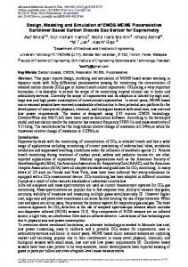
A timer is set and then a 200kHz pulse is transmitted, indicated by the first low in Figure 6, by the sensor. This time is recorded by the microcontroller. The sensor then waits for the return pulses, indicated by the subsequent lows in Figure 1, and records the time of the first of these low states. The rest of the low states are the non-direct multipath echoes that cannot be used for measurement. The time difference between the two times recorded is used, with the speed of sound in water, to determine the distance an object is from the sensor. The time difference between the pulses is recorded with a resolution of 238.4 ns allowing the sensor to be theoretically very accurate. Figure 7 shows the results of testing the custom made sensor in a fresh water environment. Time of Flight for Signal vs distance 20000

Figure 5. Sonar sensor The transducers of the sensors are linked to a control circuit board that provides simple transmitter and receiver capabilities, such as amplification and detection of the signal. The circuit board is only required to detect a returned echo. It does this by having an output that will be in a low state when a 200 kHz frequency is detected and is high otherwise. This circuit board conveys the detection output to the Motorola microcontroller onboard the Eyebot unit. Most of the distance processing is accomplished using the Eyebot’s microcontroller. The advantage of using the microcontroller is that it has a module that can time the occurrence of events. The microcontroller is programmed to record the absolute times of the transmission pulse and the first received pulse from the circuit board.

Time of flight (counts)

18000 16000 14000 12000 10000 8000 6000 4000 2000 0 0

1

2

3

4

Distance to wall (m)

Figure 7. Time of flight over a range of distances for the echo sounder (where one count is 238.4ns) To achieve a network of these sensors, the detection output from each of the sensors can be linked to one of many inputs to the timer module of the microcontroller. The input to the sensors that will activate them can be all linked to the one digital output from the microcontroller. This will enable the echo sounding sensors to operate simultaneously. The benefit of this is that the first returned pulse to the sensor is guaranteed to be that sensor’s signal, and not cross talk from other sensors. This is ensured by the fact that the non-direct cross talk will always take longer in time to be received than the direct true signal.

A simple dual water detector circuit connected to analogue-to-digital converter (ADC) channels on the Eyebot controller is used to detect the unlikely but possible event of a hull breach. Two probes run along the bottom of each hull. This allows for the location (upper or lower hull) of the leak to be known, therefore saving time in isolating a leak. The Eyebot periodically monitors whether or not the hull integrity of the vehicle has been compromised, and if so immediately surfaces the vehicle. To ensure adequate power is being supplied to the vehicle, particularly to the motors, a simple power monitor is used to detect when the voltage level drops to unacceptable levels. This is essential as a low voltage will result in the thrust characteristics of the motors drifting from expected values, therefore compromising accurate control of the vehicle. The power monitor is essentially a voltage divider circuit that connects to an ADC channel on the Eyebot. This allows the Eyebot to periodically monitor the supply voltage and to surface the vehicle when it senses a low voltage.

where M is a mass and inertia matrix, C (V ) is a Coriolis and centripetal terms matrix, D (V ) is a hydrodynamic damping matrix, G is the gravitational and buoyancy vector, T is the external force and torque input vector, and V is the velocity state vector. Note that the equation does not take into account environmental forces. The dynamic model is quite complex and obtaining many of the parameters is a very time consuming and difficult process. Therefore, simplification of the model was required. The following assertions were made for the dynamics of the Mako in order to simplify the modeling: • The vehicle travels at low speeds, that is, less than 2m/s • Roll and pitch movement is passively controlled and therefore, considered to be negligible • The vehicle is considered to be fairly symmetrical about its three planes • During all manoeuvres the vehicle is always maintained in a horizontal posture

The vision system consists of the mini PC connected to a standard parallel port web camera. The PC was mounted onto the component boards along with the other electronic components. A chassis made from Perspex and aluminium was built to house the camera in a watertight enclosure. The chassis was attached to the underside of the vehicle’s frame (Figure 3.14) so that the camera was pointing directly downwards. A through-hull connection was then made for connecting the camera to the PC located in the upper hull.

• Disturbances from the water environment on the vehicle such as currents and waves are negligible • Sway, that is, movement along the vehicle’s y axis, is negligible • The vehicle’s degrees of freedom are decoupled By assuming decoupling between the degrees of freedom, that is, assuming that motion along or about one degree of freedom does not affect another degree of freedom, the dynamic model of an AUV can be significantly simplified. According to Ridao et al. [17], the justification for the decoupling of the degrees of freedom is based on the fact that:

Figure 8. Mako camera III. AUV MODELING The Mako was modeled using a simplified underwater robotic dynamic model proposed by Fossen [15] and Yuh [16]. The dynamic model is derived from the Newton-Euler motion equation and is given by,

MV& + C (V )V + D(V )V + G = T

•

The vehicle is fairly symmetrical about its three planes

•

The off diagonal elements of the dynamic model matrices are much smaller than their counterparts

•

The hydrodynamic damping coupling is negligible at low speeds

Since the Mako is considered to be fairly symmetrical and travels at a low speed, the decoupling for the vehicle’s degrees of freedom is valid. The decoupling means that the Coriolis and centripetal terms matrices become negligible and consequently can be eliminated from the dynamic model. The simplified dynamic model for the AUV then becomes,

MV& + D(V )V + G = T This means that only the inertial and damping parameters need to be identified for the Mako.

IV.

SYSTEM IDENTIFICATION

The system identification of an AUV is quite complex and requires complete state knowledge, as well as highly complex and expensive equipment [18]. Moreover, the highly configurable and modular nature of the Mako would demand system identification of the vehicle more frequently than usual. Therefore, a methodology had to be used that would allow system identification to be relatively simple and not time consuming, as well as not requiring complex and expensive equipment.

Since it has been established that the Mako can be modelled as a symmetric and decoupled AUV, then this means that each degree of freedom can be treated separately. In this case, the simplified dynamic model can then be modified to one applicable to each degree of freedom [19],

An approach by Indiveri [18] for identifying an underwater robotic system’s dynamic model exploits some of the characteristics of the vehicle and utilises onboard sensors to successfully and easily identify the vehicle’s parameters. The approach assumes decoupling between the degrees of freedom. In the system identification, a combination of static and dynamic experiments are performed with the parameters for each degree of freedom then estimated via least squares estimation utilising the experimental data obtained. This approach was chosen for the Mako’s system identification due to its simple nature and low loss of information.

where mξ represents the inertial parameters, d ξ and the linear and quadratic damping parameters respectively, g ξ the gravitational/buoyancy force, τ ξ the input force/torque and ξ the velocity component for the particular degree of freedom. From the previous equation mξ consists of both a rigid body parameter, mRB ,ξ , and an added mass parameter, m A,ξ .

mξ ξ& + dξ ξ + dξ ξ ξ ξ + gξ = τ ξ dξ ξ

System identification of the Mako’s surge, heave and yaw degrees of freedom for both positive and negative motion using onboard sensors was attempted. The results are shown in Table 1. The shortcomings of the sensor suite prevented some values from being ascertained.

The above methodology assumes decoupling between the vehicle’s degrees of freedom. Degree of Freedom

Positive Surge

Rigid Body Mass and Inertia Parameter

Added Mass Parameter

mRB ,ξ

m A,ξ

mRB ,u

+

(kg)

35.3 Negative Surge

mRB ,u

(kg)

mRB ,w

(kg)

mRB ,w mRB ,r

−

(kg)

−

(kg)

m A, w

+

(kg)

m A, w

−

(kg)

[3.53, 35.3] *

m A,r

(kgm2)

mRB ,r

m A,u

+

3.9 ** Negative Yaw

(kg)

[3.53, 35.3] *

35.3 Positive Yaw

+

[3.53, 35.3] * +

35.3 Negative Heave

gξ

[3.53, 35.3] * −

35.3 Positive Heave

m A,u

Gravitational and Buoyancy Parameter

+

(kgm2)

[0.39, 3.9] * −

(kgm2)

3.9 **

m A,r

−

(kgm2)

[0.39, 3.9] *

* This indicates the range of values that the added mass parameter can attain. ** This value represents an upper bound on the moment of inertia.

Table 1. Mako model properites

gu

+

(N)

(N)

+

(N)

-15.1

gw

du

−

−

(N)

+

(Ns/m)

dw dw

0

dr

(Ns/m)

(N)

dr 3.2

−

du u

(Ns2/m2)

−

dw w

+

(Ns2/m2)

196.7 (Ns/m)

dw w

−

(Ns2/m2)

-+

(Nms/rad)

3.6 −

(Ns2/m2)

-+

-(N)

+

du u 67.7

26.0

15.1

0

(Ns/m)

--

gw

gr

+

16.8 −

0

gr

du

Quadratic Damping Parameter

dξ ξ

dξ

0

gu

Linear Damping Parameter

dr r

+

(Nms2/rad2)

1.8 −

(Nms/rad)

dr r 2.0

−

(Nms2/rad2)

V. SIMULATION SYSTEM There are many advantages to having a simulation system. Simulation allows concurrent development of the hardware platform and control software, reducing the time required to build a complete solution. It also enables groups who have financial or physical limitations (such as the lack of an appropriately sized body of water) to compete. Finally, simulations allow far greater control over the environment in which the submarine is placed. This simplifies the testing of a program’s performance in varied conditions. A. Software design The simulation software is designed to address a broad variety of users with different needs, such as the structure of the user interface, levels of abstraction, and the complexity of physical and sensor models. As a result, the most important design goal for the software is to produce a simulation tool that is as extensible and flexible as possible. Therefore, the entire system was designed with a plug-in based architecture from the ground up. Entire components, such as the end-user API, the user interface and the physical simulation library can be exchanged to accommodate the users’ needs. This allows the user to easily extend the simulation system by adding custom plug-ins written in any language supporting dynamic libraries, such as standard C or C++. Further goals include ease of use, portability, execution speed, and the resulting size of the distribution binary. Figure 5 shows the basic architecture of the simulation system. The simulation system provides a software developer kit (SDK) that contains the framework for plug-in development, and tools for designing and visualizing the submarine. The software packages used to create the simulator include:

The PAL allows custom plug-ins to be incorporated to the existing library, allowing custom sensor and motor models to replace, or supplement the existing implementations.

wxWidgets [9] (formerly wxWindows) – A mature and comprehensive open source cross platform C++ GUI framework. This package was selected as it greatly simplifies the task of cross platform interface development. It also offers straightforward plug-in management and threading libraries.

1) Propulsion Model The motor model implemented in the simulation is based off the standard armature controlled DC motor model [12]. The transfer function for the motor in terms of an input voltage (V) and output rotational speed (θ) is:

Figure 9. SubSim architecture

TinyXML [10] is a C++ XML parser. It was chosen over other XML parsing packages as it is simple to use, and is small enough to distribute with the simulation. The user can select the physics libraries used by the simulator. However the default physics simulation system employed is the Newton Game Dynamics engine [11], which implements a fast and stable deterministic solver. B. Physics Models The underlying low-level physical simulation library is responsible for calculating the position, orientation, forces, torques and velocities of all bodies and joints in the simulation. Since the low-level physical simulation library performs most of the physical calculations, the higher-level physics abstraction layer (PAL) [14] is only required to simulate motors and sensors.

θ V

=

K ( Js + b)( Ls + R) + K ²

Where: J is the moment of inertia of the rotor, b is the damping ratio of the mechanical system, L is the rotor electrical inductance, R is the terminal electrical resistance, and K is the electro motive force const The default thruster model implemented is based on the lumped parameter dynamic thruster model developed by D. R. Yoerger et al. [8].

The thrust produced is governed by:

Thrust = Ct Ω |Ω|

Where Ω is the propeller angular velocity, and Ct is the proportionality constant. Simulation of control surfaces is also supported. The model used to determine the lift from diametrically opposite fins [13] is given by:

L fin =

1 ρC Lδf S fin δ e ve ² 2

Where: Lfin is the lift force, ρ is the density, CLδf is the rate of change of lift coefficient with respect to fin effective angle of attack, Sfin is the fin platform area, δe is the effective fin angle,

v e is the effective fin velocity The drag forces affecting the underwater body are calculated from:

1 D = ρ .C . A .V ² 2 D

f

Where D is the drag force, ρ is the density, CD is the drag coefficient, Af is the frontal area of the body, V is the realtive velocity. 2) Simplified Propulsion Model One of the design goals of the simulation system is to ensure ease of use. To assist in accomplishing this goal, a much simpler model for the propulsion system is also provided, in the form of an interpolated look-up table. This allows a user to experimentally collect input values and measure the resulting thrust force, applying these forces directly to the submarine model. 3) Sensor Models The PAL already simulates a number of sensors. Each sensor can be coupled with an error model to allow the user to simulate a sensor that returns data similar to the accuracy of the physical equipment they are trying to simulate. Many of the positional and orientation sensors can be directly modeled from the data available from the lower level physics library. Every sensor is attached to a body that represents a physical component of an AUV.

The simulated inclinometer sensor calculates its orientation from the orientation of the body that it is attached to, relative to the inclinometers own initial orientation. Similarly, the simulated gyroscope calculates its orientation from the attached body’s angular velocity, and its own axis of rotation. The velocimeter calculates the velocity in a given direction from its orientation axis and the velocity information from the attached body. Contact sensors are simulated by querying the collision detection routines of the low-level physics library for the positions where collisions occurred. If the collisions queried occur within the domain of the contact sensors, then these collisions are recorded. Distance measuring sensors, such as echo-sounders and Positional Sensitive Devices (PSDs) are simulated by traditional ray casting techniques, provided the low level physics library supports the necessary data structures. A realistic synthetic camera image is being generated by the simulation system as well. With this, user application programs can use image processing for navigating the simulated AUV. Camera user interface and implementation are similar to the EyeSim mobile robot simulation system [4]. 4) Environment Model Detailed modeling of the environment is necessary to recreate the complex tasks facing the simulated AUV. Dynamic conditions force the AUV to continually adjust its behavior. E.g. introducing (ocean) currents causes the submarine to permanently adapt its position, poor lighting and visibility decreases image quality and eventually adds noise to PSD and vision sensors. The terrain is an essential part of the environment as it defines the universe the simulation takes part in as well as physical obstacles the AUV may encounter. 5) Error Models Like all the other components of the simulation system, error models are provided as plug-in extensions. All models either apply characteristic, random, or statistically chosen noise to sensor readings or the actuators control signal. We can distinguish two different types of errors: Global errors and local errors. Global errors, such as voltage gain, affect all connected devices. Local errors only affect a certain device at a certain time. In general local errors can be data dropouts, malfunctions or device specific errors that occur when the device constraints are violated. For example, the camera can be affected by a number of errors such as detector, Gaussian, and salt and pepper noise. Voltage gains (either constant or time dependent) can interfere with motor controls as well as sensor readings. Peculiarities of the medium the simulation is running in have to be considered, e.g. refractions due to glass/water transitions and condensation due to temperature differences on optical instruments inside the hull.

C. API The simulation system implements two separate application programmer interfaces (APIs). The first API is the internal API, which is exposed to developers so that they can encapsulate the functionality of their own controller API. The second API is the RoBIOS API, a user friendly API that mirrors the functionality present on the Eyebot [5] controller found on the Mako. The internal API consists of only five functions: SSID InitDevice(char *device_name); SSERROR QueryDevice (SSID device, void *data); SSERROR SetData(SSID device, void *data); SSERROR GetData(SSID device, void *data); SSERROR GetTime(SSTIME time);

The function InitDevice initializes the device given by its name and stores it in the internal registry. It returns a unique handle that can be used to further reference the device (e.g. sensors, motors). QueryDevice stores the state of the device in the provided data structure and returns an error if the execution failed. GetTime returns a time stamp holding the execution time of the submarines program in ms. In case of failure an error code is returned. The functions that are actually manipulating the sensors and actuators and therefore affect the interaction of the submarine with its environment are either the GetData or SetData function. While the first one retrieves the data (e.g. sensor readings) the later one changes the internal state of a device by passing control and/or information data to the device. Both return appropriate error codes if the operation fails. As mentioned earlier, an AUV application program would normally be programmed using a high level API, such as the RoBIOS system functions [2]. This allows a normal C or C++ program to be compiled with the RoBIOS library and provides all high-level functions such as motor control, reading of sensor or camera data, etc. However, since the high-level API is just a plug-in, it can be easily exchanged for any other API interface. All that needs to be done is "implementing" the new API through the low-level API primitives.. VI. CONCLUSION Our prototype AUV gives a guideline for interested parties to build their own AUV, while the simulation system provides a powerful tool in assisting the development of autonomous behavior. SubSim offers a comprehensive, yet easy to use simulation system for a variety of applications and users.

ACKNOWLEDGMENT The authors would like to thank Raytheon Australia and DSPComm Perth for their sponsorship for parts of this project. REFERENCES [1] T. Bräunl, "Embedded Robotics", Springer-Verlag Heidelberg, 2003. [2] AUVSI and ONR's 7th International Autonomous Underwater Vehicle Competition, http://www.auvsi.org/ competitions/water.cfm [3] T. Bräunl, Research relevance of Mobile Robot Competitions, IEEE Robotics and Automation Magazine, vol. 6, no. 4, Dec. 1999, pp. 32-37 (6) [4] T. Bräunl, Embedded Robotics – Mobile Robot Design and Applications with Embedded Systems, Springer-Verlag, Heidelberg, 2003 [5] T. Bräunl, UWA Mobile Robot Lab, http://robotics.ee.uwa.edu.au [6] Proceedings of 7th RoboCup International Symposium, Padua, Italy, 2003 [7] Proceedings of the FIRA Robot World Congress 2003, Wien, Oct. 2003 [8] D. R. Yoerger, J. G. Cooke, J. E. Slotine, “The Influence of Thruster Dynamics on Underwater Vehicle Behavious and Their Incorporation Into Control System Design,” IEEE J. Oceanic Eng., vol 15, no. 3, pp. 167-178, 1991. [9] WX Widgets, http://www.wxwidgets.org/ [10] Tiny XML, http://tinyxml.sourceforge.net/ [11] Newton Game Dynamics Engine, http://www.physicsengine.com/ [12] R.C. Dorf, R.H. Bishop, Modern Control Systems, Prentice-Hall, 2001, Ch. 4, pp174-223. [13] P. Ridley, J. Fontan, P. Corke, Submarine Dynamic Modeling, Australasian Conference on Robotics and Automation, 2003, CD-ROM Proceedings, ISBN 0-9587583-5-2 [14] PAL, http://pal.sourceforge.net/ [15] T. Fossen. Guidance and Control of Ocean Vehicles. John Wiley and Sons, United States of America, 1995. [16] J. Yuh. Modeling and control of underwater robot vehicles. In IEEE Transactions on Systems, Man and Cybernetics, volume 20, pages 1475–1483, 1990. [17] P. Ridao et al. Model identification of a low-speed uuv. In Control Applications in Marine Systems. International Federation on Automatic Control, 2001. [18] G. Indiveri. Modelling and Identification of Underwater Robotics Systems. PhD thesis, University of Genova, 1998. [19] M. Caccia et al. Modeling and identification of open-frame variable configuration unmanned underwater vehicles. In IEEE Journal of Oceanic Engineering, volume 25, pages 227–240, 2000.