Proceedings of the American Control Conference Arlington, VA June 25-27, 2001
Design of a class of reduced order unknown inputs nonlinear observer for fault diagnosis D. Koenig and S. Mamma* Laboratoire dAutomatique de Grenoble (UMR CNRS-INPG-UJF) BP 46,38402 SAINT MARTIN DHERES CEDEX, FRANCE * INRETS, 2 av. du GBn6ral Malleret-Joinville BP 34 - 94114 ARCEUIL, FRANCE
[email protected],
[email protected]
Abstract: In this paper the problem of fault detection in non-linear systems is considered. Our goal is to extend the unknown inputs observer approach to nonlinear systems. The approach consists of two stages. At first stage, a change of coordinates is found that decoupages the nonlinear system into two subsystems: one which is independent of the unknown inputs and another with the states that can be expressed as linear combinations of the outputs and the states of the first subsystem. Secondly a nonlinear observer is designed for the former. The use of such observer in robust fault detection purposes is then discussed, and finally illustrated by a numerical example. Keywords: Fault detection, robustness, systems and observers.
The problem is stated in section 2. Section 3 gives presents the equivalent disturbance decoupled system and section 4 gives the observer design. The stability issue is discussed in section 5 while section 6 gives its possible application to fault detection, with an illustrative example in section 7.
2 PROBLEM STATEMENT We consider a class of nonlinear systems described by
-x = A & + B g + E d + f b , g )
nonlinear
1 INTRODUCTION A critical issue in the application of observer based approaches to fault detection is the consideration of nonlinear models. Most of the research on fault detection has been dedicated to linear systems, see for example [3,5,8, 151. However, the application of linear approaches is limited if the system to be monitored is strongly nonlinear.
where
&E
y, Sn, g~ S n u-
(1.2)
and
G E Sp denotes
respectively the state, the input, the output and the unknown input vectors. Each component of the is a nonlinear function of the nonlinearity f b , g) E states and the inputs. Then following notations will be used
Notations h( ) : an eigenvalue CT( )
Different observer based approaches have been proposed in the literature: for example the application of nonlinear identity observers [3], the use of nonlinear distyrbance decoupling approach [12], or the approach based on algebra of functions [ 131. Nonlinear adaptive observers, bilinear observers and extensions of the fault detection filter to a class of nonlinear systems have been also proposed. For a recent survey see for example [ 11.
: singular value
E(.) : largest singular value
g(.) : smallest singular value
8 > 0 : positive parameter S ( e ) > 0 : solution of the Lyapunov equation y > 0 : Lipschitz constant (.)T : transpose
(X>’= (XTX)-’XT Moore-Penrose pseudo-inverse
Our goal is to extend the results of [111 by separating the disturbed part of the model from undisturbed one. 0-78O3-6495-3/01/$10.00 0 2001 AACC
(1.1)
y=cx -
2143
4 OBSERVER DESIGN
When the nonlinearity f@, U) verifies the Lipschitz condition:
Ilf k,E)- f
-41
2$ and the two following conditions @>
1)I.
rank(CE) = rank(E) = p
(2)
Thanks to the observability of the pair to propose as a filter a copy of the subsystem
(3) (4)
variable of the estimator:
-i = .ig + .i12til + B1g+ qfb,!) + s-'(e)ST - s Z ) ( ~ ) -
unknown input Luenberger observer: (5.1)
2 = M g + Ny
(5.2)
where Z E % ' - ~ and %E%'' denote respectively the state observer and the state estimate. The unknown matrices F, G, J, TI, M and N must be determined such that & will asymptotically converge to E .
3 DISTURBANCE DECOUPLING According to [7], the first step of the approach is to find
where z is the state
innovation term
hold for all complex s, one can design a reduced order
-Z = Fg+Gy+Jg+T,f@,u) -
SI plus an
The choice of the gain S-'(e)? is evidently suggested by the work of [6] on the observers for uniformly observable nonlinear systems, which satisfy a global Lipschitz condition. In that work, the matrix S(0) is defined as the solution of the equation:
- - ATs(e) + s(e)A - tTt + es(e) = 0
(IO)
Following [6], it is known that if the p a i r p ,
?)
is
observable, for any b o , there exists a positive definite matrix S(0) which verifies equation (10).
two linear state transformation T1 and T3 in order to separate the disturbed part of the model from the undisturbed one. Assume that condition (3) holds, then the searched
The following theorems give the existence conditions of observer (5) e (9) with notation of system (1).
transformation TI and T3 are such that TT andTT are
Theorem 1: Ifrank(CE) = rank(E) = p, then the following statements are equivalent:
respectively the orthonormal basis for the null space of
a) the pair A, C is observable
ETand
("
These matrices are given T: = Ker@
).%'"(.-P)
T; = Ker(a)T)s
b) r a n k r n i A (6)
7 = c-,
= n +p
for all complex s
%mx(m-~)
2, = A i 1 +A,&ytBlg+T,f(x,u)
=e;@+,) -
71
Proof: see appendix.
(7) Assuming the previous transformation, it has been proved in [7] that the following undisturbed model exists
E2
=I
Theorem 2: If conditions (2), (3) and (4) holds for all complex s, there exists an observer in the conventional Luenberger observer form (5) for system (1) with:
(8.1)
(8.2) (8.3)
(12)
J = & =TIB
(13)
M = (r: - E ~ ; E , )
(14)
N = EE; Proof: see relation's (5), (8) and (9).
(15)
2144
5
6
STABILITY ANALYSIS
=zl
We have now to verify that E, -z and -e(t) = g(t) - - ~ ( t ) tend toward zero and are independent of the unknown input d. In fact, one has: 61
= FE1 +TI (f (X, U)- f @,LI))
-MXE,(~)+(MT,+NC-I,)X(~) with (MT,
+ NC - I,)
RESIDUAL GENERATION
Once a set of subsystems which are robust to different groups of faults have been obtained, a residual generator is required to detect and isolate the 'faults [7]. There are several approaches to generate residuals for nonlinear systems: those based on observers (see the survey [l]), on nonlinear parity relations [ 141, on qualitative observers [16], and neural networks [4], etc. Consider the following partition of the fault distribution
mtrix: Hh = @+H*h* Let us consider the Lyapunov quadratic function:
v @ ~= g:s(e)E, ) and calculate the time derivative
(16)
;
h=cuh*
(22)
where the residual will be insensitive the fault unknown input d, whilst remaining sensitive to h*.
and
The systems (1) and (8) can be respectively rewritten as
+ BLJ+ Ed + H*h*+ f (x, E)
X = A&
(23)
+ 2gTs(e)r,(f(X,U)-f@.,U)) By substituting (10) in (17), the relation becomes
v(gl ) = -E: (eS(e)+ETEb, t 2ETS(e)T1(f (I.!)- f
el))(18)
and from condition (2), one deduce y x3(S(e)T1)~I~,Ilxl~l -:S(e)T, (fb.g)-f(i,!>)I
By
considering
[?]I=[:+),
the
[:r
regular
the inverse
52
sub-state estimation error can write:
base =
V2 = z2-1,
transformation
bT
E] and the ^
d:=k
with E:=[E E] and iiTr . For the subsystem (24), according to fact that the
(=
(9) and construct the residual as the difference between the estimated and the measured output of the subsystem
-
^
= -CbC1g1, one
[-i]=[;]g e2
=I
pair A,C is observable, one can design an observer as
r=Cz-Y(26) A generalized observer for system (23) is then given by -z = Fz + Gy- + JLJ + Tlf @, E) (27.1) ?=Mz+Ny -
(27.2)
E = LIZ+ L, y
(27.3)
-
where L, =
and L,
= T3.
The estimation errors Z1, e and the residual 1 are governed by the following equations
-2, =FE1+T,H*h*+T,(f(x!,u)-f@,u)) (28.1) g = -MEl
Substituting their last inequality into (18) gives
+2y.B(S(e)T,)~~(M)).1/6,11~ According to the second method of Lyapunov theory, the stability of the observer is ensured if:
z. = -?El
(28.2)
+(&,-T3C)
(28.3)
where ETl -T3C = 0 since TTTl=In-EE+ and T&E=O. Finally, in order to avoid cancellations of different components of the fault signals, one must ensure that rank(I',H*)= rank($) If this requirement is fulfilled, the fault will be reflected in the residual.
2145
The developed methodology is now applied to an illustrative example, which has been first considered in [ 101.
7 EXAMPLE
whereas the figure (6) shows that the approach of [IO] is not robust against d. A fault is introduced as a bias of the actuator at time t =12sec. The fault is detected shortly after its occurrence (see figure 5). d
Consider the following system [101
; ;
& = [ -2.414
2
-2.414 -1: ] - . [ ~ ~ + [ 3 + ~ ] h * + a [ 4 ~ ~ ~ ~ ~ : 1
I O
I
!=b ;$
Fig 2: Unknown input d
where: and are belonging to a SZ state space. Letting R:= t l s ( x l , ?&lo; -2&, i & 8 ; -5