observer-based reduced order controller design ... - Semantic Scholar

International Journal of Computer Science, Engineering and Information Technology (IJCSEIT), Vol.1, No.5, December 2011

OBSERVER-BASED REDUCED ORDER CONTROLLER DESIGN FOR THE STABILIZATION OF LARGE SCALE LINEAR DISCRETE-TIME CONTROL SYSTEMS Sundarapandian Vaidyanathan1 and Kavitha Madhavan2 1

Research and Development Centre, Vel Tech Dr. RR & Dr. SR Technical University Avadi, Chennai-600 062, Tamil Nadu, INDIA [email protected] 2

Department of Mathematics, Vel Tech Dr. RR & Dr. SR Technical University Avadi, Chennai-600 062, Tamil Nadu, INDIA [email protected]

ABSTRACT This paper discusses the design of observer-based reduced order controllers for the stabilization of large scale linear discrete-time control systems. This design is carried out via deriving a reduced-order model for the given linear plant using the dominant state of the linear plant. Using this reduced-order linear model, sufficient conditions are derived for the design of observer-based reduced order controllers. A separation principle has been established in this paper which demonstrates that the observer poles and controller poles can be separated and hence the pole-placement problem and observer design are independent of each other.

KEYWORDS Dominant State, Reduced-Order Model, Stabilization, Observers, Discrete-Time Linear System.

1. INTRODUCTION The reduced order controller design and observer design are active research problems in the linear systems literature and there has been a significant attention paid in the literature on these two problems during the past four decades [1-10]. In the recent decades, there has been a considerable attention paid to the control problem of large scale linear systems. This is mainly owing to the practical and technical issues like data acquisition, sensing, computing facilities, information transfer networks and the cost associated with them, which arise from the use of full order controller design. Thus, there is a great demand in the industry for the control of large scale linear systems with the use of reduced-order controllers rather than full-order controllers. A recent approach for obtaining the reduced-order controllers is via the reduced-order model of a linear plant preserving the dynamic as well as static properties of the system and then devising controllers for the reduced-order model thus obtained [4-8]. This approach has practical and DOI : 10.5121/ijcseit.2011.1508

85

International Journal of Computer Science, Engineering and Information Technology (IJCSEIT), Vol.1, No.5, December 2011

technical benefits for the reduced-order controller design for large-scale linear systems with high dimension and complexity. The observer-based reduced-order controller design is motivated by the fact that the dominant state of the linear plant may not be available for measurement and hence for implementing the pole placement law, only the reduced order exponential observer can be used in lieu of the dominant state of the given discrete-time linear system. In this paper, we derive a reduced-order model for any linear discrete-time control system and our approach is based on the approach of using the dominant state of the given linear discrete-time control system, i.e. we derive the reduced-order model for a given discrete-time linear control system keeping only the dominant state of the given discrete-time linear control system. Using the reduced-order model obtained, we characterize the existence of a reduced-order exponential observer that tracks the state of the reduced-order model, i.e. the dominant state of the original linear plant. We note that the reduced-order observer design detailed in this paper is a discretetime analogue of the results of Aldeen and Trinh [8] for the observer design of the dominant state of continuous-time linear control systems. Using the reduced-order model of the original linear plant, we also characterize the existence of a stabilizing feedback control law that uses only the dominant state of the original plant. Also, when the plant is stabilizable by a state feedback control law, the full information of the dominant state may not be always available. For this reason, we establish a separation principle so that the state of the exponential observer may be used in lieu of the dominant state of the original linear plant, which facilitates the implementation of the stabilizing feedback control law derived. The design of observer-based reduced order controllers for large scale discrete-time linear systems derived in this paper has important practical, industrial applications. This paper is organized as follows. In Section 2, we describe the construction of the reducedorder plant of a given linear discrete-time control system. In Section 3, we derive necessary and sufficient conditions for the exponential observer design for the reduced-order linear control plant. In Section 4, we derive necessary and sufficient conditions for the reduced-order plant to be stabilizable by a linear feedback control law and we also present a separation principle for the observer-based reduced order controller design. In Section 5, we describe a numerical example. In Section 6, we summarize the main results derived in this paper.

2. REDUCED ORDER MODEL FOR DISCRETE-TIME LINEAR SYSTEMS In this section, we consider a large scale linear discrete-time control system S1 given by

x(k + 1) = Ax (k ) + Bu (k ) y (k ) = Cx(k )

(1)

where x ∈ R n is the state, u ∈ R m is the control or input and y ∈R p is the system output. We assume that A, B and C are constant matrices with real entries having dimensions n × n, n × m p × n respectively.

First, we suppose that we have made an identification of the dominant (slow) and nondominant (fast) states of the original linear system (1) using the modal approach as described in [9]. Without loss of generality, we may assume that 86

International Journal of Computer Science, Engineering and Information Technology (IJCSEIT), Vol.1, No.5, December 2011

 xs  x =  , xf  where xs ∈ R r represents the dominant state and x f ∈ R n − r represents the non-dominant state of the system. Then the linear system (1) becomes

 xs (k + 1)   Ass  x ( k + 1)  =  A  f   fs y ( k ) = Cs

Asf   xs ( k )   Bs  + u (k ) Aff   x f ( k )   B f 

 xs ( k )  C f     x f (k ) 

(2)

From (2), we can write the plant equations as

xs (k + 1) = Ass xs (k ) + Asf x f (k ) + Bs u (k ) x f (k + 1) = Afs xs (k ) + Aff x f (k ) + B f u (k )

(3)

y (k ) = Cs xs (k ) + C f x f (k ) Next, we shall assume that the matrix A has a set of n linearly independent eigenvectors. In most practical situations, the matrix A has distinct eigenvalues and this condition is immediately satisfied. Thus, it follows that A is diagonalizable. Thus, we can find a non-singular (modal) matrix P consisting of n linearly independent eigenvectors of A such that

P −1 AP = Λ, where Λ is a diagonal matrix consisting of the n eigenvalues of A. Now, we introduce a new set of coordinates on the state space given by

ξ = P −1 x

(4)

In the new coordinates, the plant (1) becomes

ξ (k + 1) = Λξ (k ) + P −1Bu (k ) y ( k ) = CPξ (k ) Thus, we have

87

International Journal of Computer Science, Engineering and Information Technology (IJCSEIT), Vol.1, No.5, December 2011

 ξ s ( k + 1)   Λ s 0   ξ s ( k )  −1 ξ ( k + 1)  =  0 Λ  ξ ( k )  + P Bu ( k ) f  f  f     ξ s (k )  y ( k ) = CP   ξ f (k ) 

(5)

where Λ s and Λ f are r × r and ( n − r ) × ( n − r ) diagonal matrices respectively, consisting of the dominant and non-dominant eigenvalues of A. Define matrices Γ s , Γ f , Ψ s and Ψ f by

 Γs  P −1 B =   and CP =  Ψ s Γ f 

Ψ f 

(6)

where Γ s , Γ f , Ψ s and Ψ f are r × m, (n − r ) × m, p × r and p × ( n − r ) matrices respectively. From (5) and (6), we see that the plant (3) has the following simple form in the new coordinates (4).

ξ s (k + 1) = Λ sξ s (k ) + Γ s u (k ) ξ f (k + 1) = Λ f ξ f (k ) + Γ f u (k )

(7)

y ( k ) = Ψ sξ s ( k ) + Ψ f ξ f ( k ) Next, we make the following assumptions: (H1) As k → ∞, ξ f ( k + 1) ≈ ξ f ( k ), i.e. ξ f takes a constant value in the steady-state. (H2) The matrix I − Λ f is invertible. Then it follows from (7) that for large values of k , we have

ξ f ( k ) ≈ Λ f ξ f (k ) + Γ f u ( k ) i.e.

ξ f (k ) ≈ ( I − Λ f )−1 Γ f u (k )

(8)

Substituting (8) into (7), we obtain the reduced-order model of the linear plant (1) in the ξ coordinates as

ξ s (k + 1) = Λ sξ s (k ) + Γ s u (k ) y (k ) = Ψ sξ s (k ) + Ψ f ( I − Λ f )−1 Γ f u (k )

(9)

88

International Journal of Computer Science, Engineering and Information Technology (IJCSEIT), Vol.1, No.5, December 2011

To obtain the reduced-order model of the linear plant (1) in the x coordinates, we proceed as follows. By the linear change of coordinates (4), it follows that

ξ = P −1 x = Qx. Thus, we have

 ξ s (k )   xs (k )   Qss ξ (k )  = Q  x (k )  = Q  f   f   fs

Qsf   xs (k )  Q ff   x f (k ) 

(10)

Using (9) and (10), it follows that

ξ f (k ) = Q fsξ s (k ) + Q ff ξ f (k ) = ( I − Λ f )−1 Γ f u (k ) or

Q ff ξ f (k ) = −Q fs xs (k ) + ( I − Λ f )−1 Γ f u (k )

(11)

Next, we assume the following: (H3) The matrix Q ff is invertible. Using the assumption (H3), the equation (11) becomes

x f (k ) = −Q −ff1Q fs xs (k ) + Q −ff1 ( I − Λ f )−1 Γ f u (k )

(12)

To simplify the notation, we define the matrices

R = −Q −ff1Q fs and S = Q −ff1 ( I − Λ f )−1 Γ f

(13)

Using (13), the equation (12) can be simplified as

x f (k ) = Rxs (k ) + Su (k )

(14)

Substituting (14) into (3), we obtain the reduced-order model S2 of the given linear system S1 as

xs (k + 1) = As∗ xs (k ) + Bs∗u (k ) y (k ) = Cs∗ xs (k ) + Ds∗u (k )

(15)

where the matrices As∗ , Bs∗ , Cs∗ and Ds∗ are defined by

89

International Journal of Computer Science, Engineering and Information Technology (IJCSEIT), Vol.1, No.5, December 2011

As∗ = Ass + Asf R Bs∗ = Bs + Asf S

(16)

Cs∗ = Cs + C f R Ds∗ = C f S

3. REDUCED ORDER OBSERVER DESIGN In this section, we state a new result that prescribes a simple procedure for estimating the dominant state of the given linear control system S1 that satisfies the assumptions (H1)-(H3) described in Section 2. Theorem 1. Let S1 be the linear system described by

x( k + 1) = Ax (k ) + Bu ( k )

(17)

y ( k ) = Cx( k )

Under the assumptions (H1)-(H3), the reduced-order model S 2 of the linear system S1 can be obtained (see Section 2) as

xs (k + 1) = As∗ x(k ) + Bs∗u (k )

(18)

y (k ) = Cs∗ x(k ) + Ds∗u (k ) where As∗ , Bs∗ , Cs∗ and Ds∗ are defined as in (16).

To estimate the dominant state xs of the system S1 , consider the candidate observer S3 defined by

zs ( k + 1) = As∗ zs ( k ) + Bs∗u ( k ) + K s∗  y (k ) − Cs∗ zs (k ) − Ds∗u (k ) 

(19)

Let the estimation error be defined as

e = zs − xs Then e( k ) → 0 exponentially as k → ∞

E = As∗ − K s∗Cs∗ is convergent. If

if and only if the matrix K s∗ is such that

( C , A ) is observable, ∗ s

∗ s

then we can always construct an

exponential observer of the form (19) having any desired speed of convergence. Proof. From Eq. (2), we have

xs (k + 1) = Ass xs (k ) + Asf x f (k ) + Bs u (k )

(20)

Adding and subtracting the term ( Asf − K s∗C f ) Rxs ( k ) in the RHS of Eq. (20), we get 90

International Journal of Computer Science, Engineering and Information Technology (IJCSEIT), Vol.1, No.5, December 2011

xs ( k + 1) = ( Ass + Asf R − K s∗C f ) xs (k ) + Asf x f ( k ) − ( Asf − K s∗C f ) Rxs (k ) + Bs u (k )

(21)

Subtracting (21) from (19) and simplifying using the definitions (16), we get

e(k + 1) = ( As∗ − K s∗Cs∗ )e(k ) − ( Asf − K s∗C f )[ x f (k ) − Rxs (k ) − Su (k )]

(22)

As proved in Section 2, the assumptions (H1)-(H3) yield x f ( k ) ≈ Rxs ( k ) + Su (k )

(23)

Substituting (23) into (22), we get

e(k + 1) = ( As∗ − K s∗Cs∗ )e(k ) = Ee(k )

(24)

which yields e( k ) = ( As∗ − K s∗Cs∗ ) k e(0) = E k e(0)

(25)

From Eq. (25), it follows that e( k ) → 0 as k → ∞ if and only if E is convergent.

(

)

If Cs∗ , As∗ is observable, then it is well-known [10] that we can find an observer gain matrix K s∗ that will arbitrarily assign the eigenvalues of the error matrix E = As∗ − K s∗Cs∗ . In particular, it follows from Eq. (25) that we can find an exponential observer of the form (19) having any desired speed of convergence.

4. OBSERVER-BASED REDUCED ORDER CONTROLLER DESIGN In this section, we first state an important result that prescribes a simple procedure for stabilizing the dominant state of the reduced-order linear plant derived in Section 2. Theorem 2. Suppose that the assumptions (H1)-(H3) hold. Let S1 and S 2 be defined as in Theorem 1. For the reduced-order model S2 , the state feedback control law

u (k ) = − Fs∗ xs (k )

(26)

stabilizes the dominant state xs of the reduced-order model S2 having any desired speed of convergence. In practical applications, the dominant state xs of the reduced-order model S2 may not be directly available for measurement and hence we cannot implement the state feedback control law (26). To overcome this practical difficulty, we derive an important theorem, usually called as the Separation Principle, which first establishes that the observer-based reduced-order controller indeed stabilizes the dominant state of the given linear control system S1 and also demonstrates that the observer poles and the closed-loop controller poles can be separated.

91

International Journal of Computer Science, Engineering and Information Technology (IJCSEIT), Vol.1, No.5, December 2011

Theorem 3 (Separation Principle). Suppose that the assumptions (H1)-(H3) hold. Suppose that there exist matrices Fs∗ and K s∗ such that As∗ − Bs∗ Fs∗ and As∗ − K s∗Cs∗ are both convergent matrices. By Theorem 1, we know that the system S3 defined by (19) is an exponential observer for the dominant state xs of the control system S1 . Then the observer poles and the closed-loop controller poles are separated and the control law

u (k ) = − Fs∗ zs (k )

(27)

also stabilizes the dominant state xs of the control system S1. Proof. Under the feedback control law (27), the observer dynamics (19) of the system S3 becomes

(

)

zs ( k + 1) = As∗ − Bs∗ Fs∗ − K s∗Cs∗ − K s∗ Ds∗ Fs∗ zs ( k ) + K s∗ Cs xs (k ) + C f x f ( k )  (28) By (14), we know that

x f (k ) ≈ Rxs (k ) + Su (k ) = Rxs (k ) − SFs∗ zs (k )

(29)

Substituting (29) into (28) and simplifying using the definitions (16), we get

zs (k + 1) = ( As∗ − Bs∗ Fs∗ − K s∗Cs∗ ) zs (k ) + K s∗Cs∗ xs (k )

(30)

Substituting the control law (27) into (3), we also obtain

xs ( k + 1) = As∗ xs ( k ) − Bs∗ Fs∗ zs ( k )

(31)

In matrix representation, we can write equations (30) and (31) as

 xs (k + 1)   As∗  z (k + 1)  =  ∗ ∗  s   K s Cs

  xs ( k )  − Bs∗ Fs∗  ∗ ∗ ∗ ∗ ∗ As − Bs Fs − K s Cs   zs (k ) 

(32)

Since the estimation error e is defined by e = z s − xs , it is easy to see from equation (32) that the error e satisfies the equation

(

)

e( k + 1) = As∗ − K s∗Cs∗ e( k )

(33)

Using the ( x, e) coordinates, the composite system (32) can be simplified as

 xs (k + 1)   As∗ − Bs∗ Fs∗  e (k + 1)  =  0  s  

− Bs∗ Fs∗   xs (k )   =M As∗ − K s∗Cs∗   es (k ) 

 xs ( k )   e (k )   s 

(34)

where

92

International Journal of Computer Science, Engineering and Information Technology (IJCSEIT), Vol.1, No.5, December 2011

 A∗ − Bs∗ Fs∗ M = s 0 

− Bs∗ Fs∗  . As∗ − K s∗Cs∗ 

(35)

Since the matrix M is block-triangular, it is immediate that

(

)

(

eig( M ) = eig As∗ − Bs∗ Fs∗ U eig As∗ − K s∗Cs∗

)

(36)

which establishes the first part of the Separation Principle namely that the observer poles are separated from the closed-loop controller poles. To show that the observed-based control law (27) indeed works, we note that the closed-loop regulator matrix As∗ − Bs∗ Fs∗ and As∗ − K s∗Cs∗ are both convergent matrices. From Eq. (36), it is immediate that M is also a convergent matrix. From Eq. (35), it is thus immediate that xs ( k ) → 0 and es (k ) → 0 as k → ∞ for all xs (0) and e(0).

5. NUMERICAL EXAMPLE In this section, we consider a fourth-order linear discrete-time control system described by

x(k + 1) = A x( k ) + B u (k ) y (k ) = Cx(k )

(37)

where

 2.0  0.4 A=  0.1  0.7

0.6 0.2 0.3 1  1 0.4 0.9 0.5 , B =   and C = [1 2 1 1] . 1 0.3 0.5 0.1   0.9 0.8 0.8 1

(38)

The eigenvalues of the matrix A are

λ1 = 2.4964, λ2 = 1.0994, λ3 = 0.3203 and λ4 = −0.2161.

(39)

From (39), we note that λ1 , λ2 are unstable (slow) eigenvalues and λ3 , λ4 are stable (fast) eigenvalues of the system matrix A. For this linear system, the dominant and non-dominant states are calculated. A simple calculation using the procedure in [9] shows that the first two states { x1 , x2 } are the dominant (slow) states, while the last two states

{ x3 , x4 } are the non-dominant (fast) states for the given system (37).

Using the procedure described in Section 2, the reduced-order linear model for the given linear system (37) can be obtained as

93

International Journal of Computer Science, Engineering and Information Technology (IJCSEIT), Vol.1, No.5, December 2011

xs ( k + 1) = As∗ x( k ) + Bs∗u ( k ) y ( k ) = Cs∗ x( k ) + Ds∗u ( k )

(40)

where

 2.0077 1.1534  0.8352  As∗ =  , Bs∗ =     0.3848 1.5581 1.1653 

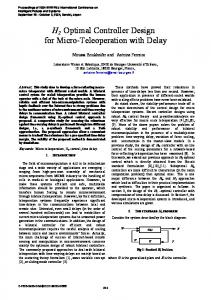
Cs∗ = [1.0092 4.0011] and Ds∗ = −0.2904 The step responses of the original plant and the reduced order plant are plotted in Figure 1, which validates the reduced-order model obtained for the given linear plant.

Figure 1. Step Responses for the Original and Reduced Order Linear Systems We note also that the reduced-order linear system (40) is completely controllable and completely observable. Thus, reduced-order observers and observer-based controllers for this plant can be easily constructed as detailed in Sections 3 and 4.

6. CONCLUSIONS In this paper, using the dominant state analysis of the given large-scale linear plant, we obtained the reduced-order model of the linear plant. Then we derived sufficient conditions for the design of observer-based reduced-order controllers. The observer-based reduced order controllers are constructed by combining the reduced order controllers for the original linear system which 94

International Journal of Computer Science, Engineering and Information Technology (IJCSEIT), Vol.1, No.5, December 2011

require the dominant state of the original system and reduced order observers for the original linear system which provide an exponential estimate of the dominant state of the original linear system. We also established a separation principle in this paper which shows that the pole placement problem and observer problem are independent of each other.

REFERENCES [1]

Cumming, S.D. (1969) “Design of observers for reduced dynamics”, Electronics Letters, Vol. 5, pp 213-214.

[2]

Fortman, T.E. & Williamson, D. (1971) “Design of low-order observers for linear feedback control laws”, IEEE Trans. Automat. Control, Vol. 17, pp 301-308.

[3]

Litz, L. & Roth, H. (1981) “State decomposition for singular perturbation order reduction – a modal approach”, Internat. J. Control, Vol. 34, pp. 937-954.

[4]

Lastman, G. & Sinha, N. & Rozsa, P. (1984) “On the selection of states to be retained in reducedorder model”, IEE Proc. Part D, Vol. 131, pp 15-22.

[5]

Anderson, B.D.O. & Liu, Y. (1989) “Controller reduction: concepts and approaches”, IEEE Trans. Automat. Control, Vol. 34, pp 802-812.

[6]

Mustafa, D. & Glover, K. (1991) “Controller reduction by H∞ balanced truncation”, IEEE Trans. Automat. Control, Vol. 36, pp 668-692.

[7]

Aldeen, M. (1991) “Interaction modelling approach to distributed control with application to interconnected dynamical systems”, Internat. J. Control, Vol. 241, pp 303-310.

[8]

Aldeen, M. & Trinh, H. (1994) “Observing a subset of the states of linear systems”, IEE Proc. Control Theory Appl., Vol. 141, pp 137-144.

[9]

Sundarapandian, V. (2005) “Distributed control schemes for large scale interconnected discrete-time linear systems”, Math. Computer Modelling, Vol. 5, pp 313-319.

[10] Ogata, K. (2010) Discrete-Time Control Systems, Prentice Hall, New Jersey.

Authors Dr. V. Sundarapandian obtained his Doctor of Science degree in Electrical and Systems Engineering from Washington University, Saint Louis, USA under the guidance of Late Dr. Christopher I. Byrnes (Dean, School of Engineering and Applied Science) in 1996. He is currently Professor in the Research and Development Centre at Vel Tech Dr. RR & Dr. SR Technical University, Chennai, Tamil Nadu, India. He has published over 210 refereed international publications. He has published over 100 papers in National Conferences and over 50 papers in International Conferences. He is the Editor-in-Chief of International Journal of Mathematics and Scientific Computing, International Journal of Instrumentation and Control Systems, International Journal of Control Systems and Computer Modelling, etc. His research interests are Linear and Nonlinear Control Systems, Chaos Theory and Control, Soft Computing, Optimal Control, Process Control, Operations Research, Mathematical Modelling, Scientific Computing using MATLAB etc. Mrs. M. Kavitha received the B.Sc. degree in Mathematics from Bharatidasan University, Tiruchirappalli, Tamil Nadu in 1998, M.Sc. degree in Mathematics from Bharatidasan University, Tiruchirappalli, Tamil Nadu in 2000, P.G. Diploma in Computer Applications from Bharatidasan University, Tiruchirappalli, Tamil Nadu, M.Phil in Mathematics from Madurai Kamaraj University, Madurai, Tamil Nadu in 2004 and currently pursuing PhD degree in Mathematics from Vel Tech Dr. RR & Dr. SR Technical University, Chennai, India. She has 9 years of teaching experience and her thrust areas of research are Difference and Differential Equations and Linear Control Systems. 95