DESIGN OF A DIGITALLY PROGRAMMABLE DELAY-LOCKEDLOOP FOR A LOW-COST ULTRA WIDE BAND RADAR RECEIVER N. Paulino 1,2,M. Serrazina1,2, J. Goes 1,2, A. Steiger-Garção 1,2 1
UNINOVA - CRI Campus da Faculdade de Ciências e Tecnologia 2825 – 114 Monte da Caparica – PORTUGAL E-mail:
[email protected]
2
Faculdade de Ciências e Tecnologia Campus da Faculdade de Ciências e Tecnologia 2825 – 114 Caparica – PORTUGAL E-mail:
[email protected]
2. ARCHITECTURE OF THE PROGRAMABLE DLL
ABSTRACT This paper presents a digitally programmable delay line intended for use as timing generator in a RADAR ranging system. Traditional delay lines are realized selecting the delayed signal from a tap in a cascade of delay elements, resulting in a delay resolution limited by the matching errors between the delay elements. The architecture of the programmable delay line presented in this paper uses a Σ∆ modulator to generate a delay unaffected by matching and a delay locked loop to filter the excess jitter noise from the output clock. System level simulations show that it is possible to obtain a resolution of 11 bits corresponding to an average output rms jitter noise of 11.4 ps.
1. INTRODUCTION Recently, the FCC approved new regulations regarding the use of ultra wide band signals (UBW) [1]. Using these signals it is possible to build low-cost short-range RADAR ranging systems such as the one described in [2]. These systems work by measuring the travel time of a signal from the transmitter to the target and back to the receiver. In order to measure this time it is necessary to compare the received signal with a delayed version of the transmitted signal until an echo is found. The target range can be determined from this delay. Traditionally-digitally programmable delay lines are realized using a cascade of delay elements and selecting the output of the element corresponding to the desired delay. Typically this delay line is inserted into a delay-locked-loop (DLL) to guaranty that the delay is not affected by process and temperature variations. This architecture is unavoidable if several delayed versions of the master clock are needed. This type delay line suffers from element mismatch, resulting in limited delay resolution [3,4]. Another problem is that if a small delay step is required the delay line will be composed of large number of delay elements, each one with the small delay step. Normally, a delay element needs a large current to realize a small delay and as a consequence, the overall power dissipation will be large. The architecture presented in this paper is capable of generating a digitally programmable delay whose resolution is not affected by element mismatch and is only limited by the response time to a new programming code. The current in the delay elements is limited by the required jitter noise in the output clock due to the circuit’s noise (thermal and flicker).
A DLL, such as the one depicted in Fig. 1, is a feedback loop, where the delay produced by a voltage controlled delay line (VCDL) in a clock signal, is adjusted to be equal to one or more periods of the reference clock. This loop works in a similar way to a Phase Locked Loop (PLL) with the difference that the input frequency is always equal to the output frequency. The loop compares the phase (delay) of the reference clock with the phase of the delayed clock using a phase detector (PD) that, in turn, drives a charge pump (CP). The output of the CP goes trough a low-pass filter and the resulting voltage is used to control the delay in the VCDL. The loop will stop adjusting the control voltage when the rising edges of both clocks coincide. Normally the input clock of the VCDL is the same clock signal used as the reference clock. Reference clock
clock
Phase u d comp
Charge Pump
Lowpass Filter
Delayed clock Control voltage Fig. 1: Block diagram of a Delay Lock Loop.
If two different clock signals, with the same frequency, are used as the reference clock and the input clock for the VCDL, the loop will try to adjust the VCDL to produce a delay equal to the average delay between the two clock signals, that causes the rising edges of both clock signals to coincide. The reference clock does not need to be a clean signal (i.e. with low jitter noise) because the DLL will act as a low pass filter that will eliminate the excess jitter noise from the reference clock. The jitter noise from the input clock of VCDL and the jitter noise introduced by the VCDL will not be affected by the loop; the first is typically very low if a crystal oscillator is used. The rms jitter noise introduced by the VCDL can be around 2 to 7 ps by careful design it [5-7]. In this paper, this noise will not be included in the analysis because we are only interested in the jitter noise introduced by the architecture. The noisy reference clock is generated switching from the clean input master clock and a delayed version of this clock (with a fixed delay equal to
TD), as shown in Fig 2. A digital Σ∆ modulator, with a fixed input digital code, controls the switching sequence, which produces a reference clock with a large jitter noise, but with an average delay that can be controlled by the digital input code of the Σ∆ modulator. To avoid spikes in this reference clock the delay TD should be inferior to half period of the master clock. If necessary, the delay TD can be adjusted by another DLL to have an exact value. Delay
Σ∆
Delay control
DLL
TD
Master clock
Delayed clock
Noisy Ref. clock
Fig.2: Architecture of the digitally programmable DLL
This reference clock is applied to the DLL and the loop will adjust the delay produced by the VCDL in the master clock to match the average delay of the reference clock. The lowpass characteristic of the DLL will filter most of the jitter noise from the output clock. To illustrate the operation of the circuit the waveforms of these signals can be seen in Fig. 3 for the case of 50% desired delay.
where NTF is the noise transfer function of the Σ∆ modulator. This expression is equivalent to the expression of the power spectral density of the quantization noise in a Σ∆ modulator [8]. The expression shows that, due to the modulation effect of the Σ∆, the jitter noise of the reference clock is mainly in frequencies close to the clock frequency. It should be noted however that, the Σ∆, depending on the input DC level, could produce tones that can alter this ideal distribution of the jitter energy over the frequency. These tones can be reduced if a dither signal is applied to the Σ∆. The DLL loop acts as low-pass filter and reduces most of the noise energy, which is located mainly at high frequencies. The minimum order of this filter is related to the order of the Σ∆. However, the filter must be second-order because of closed-loop stability problems. The optimum order of the Σ∆ modulator can be determined calculating the rms value of the jitter noise at the output for different orders of Σ∆ modulators. The variance of the jitter noise at the output of the DLL is obtained integrating the spectral noise density of the input jitter multiplied by the squared modulus of the DLL transfer function, according to:
σ
Fixed delay (T D) Master clock
2 jitter
FCLK
2
= ∫− FCLK S (e 2
j 2π fTCLK
2
) H DLL (e
j 2π fTCLK
) df
(2)
where HDLL is the loop second order low pass transfer function with complex poles. Defining the resolution of the sys-
Delayed clock
tem as res = log 2 TD
Delay control
TD = 2 ⋅ TCLK
(σ
)
⋅ 12 and considering for TD = 100 ns the dependence of the resolujitter
tion with the closed loop frequency (fp) is shown in Fig. 4 for different orders of Σ∆ modulators.
Reference clock Output clock
20
Delay resolution (bits)
Output jitter Fig. 3: Signal Waveforms in the programmable DLL for 50% delay
In this figure, the delay control signal is ON 50% of time. The delay in this signal is TD when the control signal is ON and 0 when the control is OFF, resulting in an average delay of 0.5.TD for the delay reference clock. The DLL adjusts the delay in the VCDL to match this average delay, producing an output clock with the desired delay but with some remaining jitter.
3. OUTPUT JITTER CALCULATION The circuit of Fig. 2 can be considered as digital to analog converter (where the analog output signal is a time-delay) with one bit resolution. When the control signal is ON the delay is TD, when this signal is OFF the delay is 0. The “LSB” of this converter is TD and the spectral power density of the quantization noise can be approximated by:
S ( z ) = NTF ( z )
2
TD
2
1
12 FCLK
,
(1)
15 1st order nd 2 order 3rd order 10 5 3 10
4
10 Closed loop pole frequency (Hz)
10
4
Fig. 4: System resolution (in bits) of the DLL for different closed loop frequencies and SD order of 1,2 and 3.
From this graph one can conclude that a second order modulator produces the best resolution for a given fp. It should be noted that there is a trade-off between the fp/Fclk ratio and the system resolution, i. e., a higher resolution means a lower ratio, which translates into a higher settling time for a given Fclk. The closed loop pole quality factor (Qp) does not affect this graph as long as it is kept between 0.5 and 1.4. As an example a resolution of 11 bits, corresponding to an rms jitter of 9.2 ps, with fp=16 kHz.
4. LOOP TRANSFER FUNCTION In the previous section it was concluded that the closed-loop transfer function should have a certain pole frequency for a given resolution. To design the loop it is necessary to calculate the relation between the closed-loop parameters and the characteristics of each loop element. The frequency-phase comparator samples the delay between the two clock signals and activates the charge pump for the duration of the sampled delay (d[n]). The sample frequency is, of course Fclk. An example of the waveforms for the phase comparator is shown in Fig. 5, in this figure the inputs are signals A and B where signal B defines de sampling instant of the phase-delay between the two signals.
d [n -2 ]
B
d [n ]
d [n -1 ]
(6)
clk
C
(
)
K PD ⋅ KVCDL ⋅ H1 ( z )
(8)
1 + K PD ⋅ KVCDL ⋅ H1 ( z )
j 2π fT
CLK this transfer function is evaluated substituting z = e , but if fp is small compared to Fclk (as is the case), the frequency response can be evaluated using z = 1 + j 2π f T .
dow n ( n - 2 ) .T c lk
( n - 1 ) . T c lk
n .T c lk
up
CLK
Fig. 5: Typical waveforms in a phase-frequency comparator. This sampled delay (d[n]) controls the time duration that the current source of the CP will be ON with a constant current equal to Ip. This current will charge a capacitor (C) increasing or decreasing its voltage depending on which current source is on, which in turn is controlled by the “up” and “down” signals. The voltage in this capacitor varies with time according to: vC (t ) = vC [( n − 1) Tclk ] .e
−
t
Roff . C
( n − 1).Tclk ≤ t ≤ [ n.Tclk − d ( n ) ]
clk
τ
+ v [ n − 1] T τ
In this expression KPD is the gain of the phase detector and KVCDL is the gain of the VCDL. The frequency response of
T c lk
[ n.T
Tclk
The discrete open loop transfer function is obtained applying the Z transform to equations (5) and (6) and solving in order of Vo(z) and is given by: I p 1 −1 ⋅ z Vo ( z ) C τ = (7) H1 ( z ) = Tclk D (z) −1 −1 1 − z 1 − z 1 − τ The DLL closed loop transfer function is obtained by Mason’s rule resulting in:
H2 ( z) =
A
vC (t ) = vC
vo [ n ] = vo [ n − 1] 1 −
[( n − 1) T ] + clk
(
1−e
− d ( n ) ] ≤ t ≤ n.Tclk
−
t
RC
≈ vC [( n − 1) Tclk ]
)(
. I p . R − vC
(3)
[( n − 1 ) T ] ) clk
(4)
Equation (3) represents the capacitor voltage when the current source is off. This voltage can be considered approximately constant since the OFF resistance of the current source is very high. Equation (4) represents the capacitor voltage when the current source is ON, assuming that Tclk is very small compared to R.C (where R is ON output resistance of the current source) these two equations can be simplified to obtain: Ip vc [ n ] = vc [ n − 1] + d [ n ] . (5) C To obtain a second-order loop, it is necessary add another pole realized by a simple RC time constant. Assuming that this extra pole has a time constant equal to τ>>Tclk, the output voltage at the end of a clock period can be obtained by a similar analysis and is given by:
Using this approximation the pole quality factor and frequency are given by: fp =
1
K PD ⋅ K VCDL ⋅
2π
IP 1 ⋅ ⋅ FCLK C τ
(9)
IP 1 ⋅ ⋅ FCLK C τ I 1 ⋅ K VCDL ⋅ P ⋅ C τ
K PD ⋅ K VCDL ⋅ QP =
1
τ
+ K PD
(10)
These expressions are used to obtain the values of τ and Ip/C that produce fp = 16 kHz and Qp = 0.5. The exact and approximated closed-loop frequency responses of the loop can be observed in Fig. 6. These functions differ only for frequencies close to Fclk/2 where the exact transfer function attenuation decreases. Due to this difference, the calculated rms jitter noise value, using the exact transfer function, is equal to 12.05 ps which is slightly larger than the value predicted in the previous section. 0 20 Hdisc Hcont
40 60
80 103
104
105
Frequency (Hz)
10 6
10 7
Fig 6: Closed-loop frequency response (in dB), calculated using the exact discrete transfer function and the approximated continuous expression.
5
SYSTEM LEVEL SIMULATIONS
8
x 10
Step response
-8
4 2 0.2
x 10
0.4
0.6
0.8
-8
1
1.2
time (s)
1.4
1.6
1.8 x 10
2
-4
7.502 7.5 7.498 7.496 7.494 0.4
0.6
0.8
1
1.2
1.4
time (s)
1.6
1.8
2 -4 x 10
Fig. 7:Step response of the programmable DLL compared with the ideal system for a 75 ns final value. The bottom graphic is a magnification of the end value of the response. To verify the programming range a stair case input is applied to the control input and the output delay measured, this is shown in Fig.8. 10
x 10
Output delay (s)
-8
9 8 7 6 5 4 3 2 1 0
0
2
4
6
8
10
12
time (s)
14
2 1 0
-1 -2 -3 -4 -0.8
-0.6
-0.4
-0.2
0
0.2
0.4
0.6
0.8
1
Input code
Fig. 9 Simulated output delay error with rms jitter intervals (triangles) and peak-to-peak error intervals (squares).
From this last graph we can conclude that the output rms jitter level depends on the desired delay. The average rms jitter noise is 11.4 ps, which is in accordance with the predicted value of the previous section (12.5 ps).
6. CONCLUSIONS
6
0 0
3
seconds
The programmable DLL was modeled and several simulations were realized to validate the system design. In this simulation it was necessary to use a reset signal in the PC to guaranty convergence to the programmed delay. This reset signal is necessary because the VCDL has a limited delay adjusting range and if the PC is not properly initialized the necessary delay adjustment might be outside the VCDL adjustable range. This reset it not required in a PLL because a VCO has an infinite delay adjustment range. The VCDL was modeled as an ideal delay with a minimum delay equal to 10 ns and a maximum delay equal to TD. The transient behavior of the output delay of the system was simulated with a 75 ns step applied to the control signal and the system response is compared to the transient behavior of an ideal second order system. These two responses are depicted in Fig. 7 and there is a good adjustment between system output and the expected output, confirming the validity of expressions (9) and (10).
Delay error (o), rms jitter (∆) and peak to peak value
x 10-11 4
16
18 20 -4 x 10
Fig. 8: Output delay of the DLL for a ramp in the control delay.
Additionally, several simulations were carried out where different delays were selected. After the response of the system stabilizes, the real delay, the rms and peak-to-peak value of the jitter noise are measured. These results can be observed in Fig.9.
This paper presented a digitally programmable delay line intend for use as timing generator for a short RADAR ranging system. The architecture of the programmable delay line presented in this paper uses a Σ∆ modulator to generate a delay unaffected by matching and a delay lock loop to filter the excess jitter noise from the output clock. System level simulations show it possible to obtain a resolution of 11 bits corresponding to an average output rms jitter noise of 11.4 ps.
ACKNOWLEDGMENTS The research work that led to this implementation was partially supported by the Portuguese Foundation for Science and Technology under Single-Chip-Radar-Sensor (PRAXIS/P/EEI/12036/98) and under ADOPT (PCTI/1999/ESE/33311) Projects.
REFERENCES [1] First Report and Order (FCC 02-48). [2] McEwan, “Ultra-Wideband Receiver”, US Patent 5523760, June 1996. [3] Manuel Mota, Jorgen Christiansen, “A High-Resolution Time Interpolator Based on a Delay Locked Loop and an RC Delay Line”, IEEE J. of Solid-State Circuits, Vol. 34, No.10 October 1999. [4] R.C.H. van de Beek, E.A.M. Klumperink,C.S. Vaucher and B.Nauta, “On Jitter due to Delay Cell Mismatch in DLL-based Clock Multipliers”, in Proc.IEEE ISCAS May 2002. [5] John A. McNeil, “Jitter in Ring Oscillators”, IEEE J. of SolidState Circuits, Vol. 32, No.6 June 1997. [6] Todd C: Weigand, Beomsup Kim, Paul R. Gray, “Analysis of Timing Jitter in CMOS Ring Oscilator”, in Proc.IEEE ISCAS May 1994. [7] Chulwoo Kim, In-Chul Hwang, Sung-Mo Kang, “Low-Power Small-Area 7.28 ps Jitter 1 GHz DLL-Based Clock Generator”, ISSCC Digest of Technical Papers 2002. [8] S. Norsworthy, R. Schreier, G. Temes, “Delta-Sigma Data Converters, Theory, Design and Simulation”, IEEE PRESS