2010 IEEE International Conference on Robotics and Automation Anchorage Convention District May 3-8, 2010, Anchorage, Alaska, USA
Design of a Dynamically Stable Horizontal Plane Runner Jacob Shill†, Bruce Miller†, John Schmitt‡, and Jonathan E. Clark† †Department of Mechanical Engineering, FAMU & FSU College of Engineering, Tallahassee, FL, USA ‡School of Mechanical, Industrial and Manufacturing Engineering, Oregon State University, Corvallis, OR, USA
[email protected]
Abstract— This paper describes the development of a horizontal-plane dynamic running robot based on a reduced order locomotion model, the Lateral-Leg Spring (LLS) model. Contributions include the development of a scaled, actuated, distributed mass simulation of the model, control approaches to compensate for physical and motor limitations, and the design and fabrication of bipedal running robot that instantiates the horizontal plane dynamics of the LLS model.
I. INTRODUCTION Animals run nimbly over rough terrain and are agile over a variety of environments. Building legged robots that can reproduce their remarkable speed and stability characteristics, however, is a challenging task. The past few decades have witnessed substantial progress in the development of dynamic running robots, with recent progress aided, in part, by the use of reduced order locomotion models. While legged robots represent complex, large degree of freedom systems, the coordination required in locomotion can produce dynamics that are well characterized by a reduced order system. As a result, when constructed appropriately, these lower order models can provide insight into the design, control and behavior of their robotic counterparts. The primary two-dimensional reduced order locomotion models are the Spring-Loaded Inverted Pendulum (SLIP) [1, 2] and the Lateral-Leg Spring (LLS) models [3, 4]. The SLIP model represents sagittal plane locomotion dynamics by a simple mass-spring hybrid-dynamic system. In a similar fashion, the LLS model captures the horizontal plane lateralbouncing motions in an equally simple conservative massspring model. The SLIP model has served as an inspiration for many successful dynamic legged robots including Raibert’s hoppers, Sprawlita, ARL Monopod, and Scout among others [5, 6, 7]. While the LLS model has not yet been utilized to the same effect, LLS locomotion simulations demonstrate a striking correlation to observed insect behavior [8], thereby motivating its use in the design and development of legged robots with significant lateral plane dynamics. Lateral dynamics also have importance for runners that operate primarily in the sagittal plane. For example, the hexapedal robot RHex [9], which has demonstrated impressive mobility and SLIP-like sagittal plane dynamics [10], also evidences horizontal plane dynamics with lateral ground reaction force patterns that change with variations in its leg splay [11]. Its morphology, however, precludes active or independent control of the lateral dynamics, and the effect of these postural changes on its locomotion dynamics and stability remain un-
978-1-4244-5040-4/10/$26.00 ©2010 IEEE
known. Despite these indications that lateral plane locomotion dynamics are present and are important, no robot to date has demonstrated dynamic lateral stability through instantiation of the LLS. The conspicuous absence of LLS-based robots may be in part due to the effects of scaling. Animals that employ a laterally sprawled posture, such as cockroaches and geckoes, are typically small. As animals increase in size the ability of their limbs to generate and support large lateral loads decreases. From a robotics perspective, the size of a synthetic running platform that can benefit from the lateral stability afforded by bouncing in the manner prescribed by the LLS remains an open question. To provide insight into the importance of lateral plane dynamics, in this paper we present the design and control of a 1.5 kg horizontal plane robot that utilizes lateral pushing of the legs to stabilize its locomotion. A CAD image of the lateral plane robot considered in this study is shown in Fig. 1. In addition to horizontal running, the robot will also be able to adapt its leg motions to modulate its generation of lateral forces over a variety of slopes. As a result, the robot can also be used to investigate how and why animals change their generation of lateral forces from pushing to pulling as they transition from horizontal to vertical running [12, 13].
Fig. 1.
CAD image of the dynamically stable horizontal plane runner
The remainder of the paper is organized as follows. Section II provides a brief summary of the LLS model and describes the first contribution of the paper: the development of a scaled, distributed-mass simulation of a LLS-runner that is both energetically feasible and physically realizable. Section III describes the second contribution, a new control scheme for LLS that combines leg recirculation, energy addition and removal, and control adaptations necessary to deal with the requirements associated with physical implementation, including limitations in control authority and recirculation of massive legs. Section IV presents the results of the new control method on the locomotion of both the rigid-body LLS model and
4749
the distributed-mass robot simulation. Section V describes the final contribution of the paper: the design and fabrication of a robot that instantiates LLS dynamics. Section VI summarizes the conclusions of the paper and provides a brief discussion of future work. II. H ORIZONTAL P LANE DYNAMIC M ODEL The LLS model (see Fig. 2) represents the body unit of an animal by a rigid body with a set mass and moment of inertia. A pair of effective legs, each one representing the collective effect of the support provided by multiple legs of the animal during a stance phase, is pivoted at a point P in the body, the ‘hip’ joint. The leg attachment point is displaced distances d1 and d2 along the horizontal and vertical body axes from the center of mass, and can assume different positions in the body for left and right stance phases. Since the legs of sprawled-posture animals typically represent a small fraction of the total mass, each leg is modeled by a massless, laterally rigid, axially-elastic linear spring of unstressed length lo and constant spring stiffness.
issues including: scaling, active energy management, and leg design and placement. In order to efficiently design the robot a two-dimensional distributed mass dynamic simulation was R software with the first created using the WorkingModel 2D R control inputs calculated in Matlab . A. Scaling While animals of different scales may have radically differing physiologies or locomotion strategies, some aspects of their locomotion, including the center of mass dynamics, are often remarkably similar. The broad range of animals whose center of mass dynamics are well represented by the SLIP model for running [2] suggests that the underlying lateral dynamics may also be applicable in a range of interest which extends to the design point selected for our robot. With knowledge of the specifications of existing robots, manufacturing techniques employed, and the required electronics payload, the estimated mass of the robot to be built is 1.5 kg. The LLS model has been validated with parameters characteristic of the death-head cockroach Blaberus Discoidalis, which weighs about 2.5 g. Using these values and dynamic scaling equations enumerated by Alexander [14] and Clark, et al. [15] equivalent body and performance parameters were calculated for the horizontal plane robot, a summary of which is given in Table I. TABLE I C OMPARISON OF SCALED ROBOT PARAMETERS . Parameter Body Mass Body Inertia Rest Leg Length Leg Spring Stiffness Stride Frequency
Fig. 2. (a) LLS model definition (b) A left stance phase for the model illustrating components of the system state (velocity, heading angle, body ˙ β) at leg touch-down rotation, body angular velocity, leg angle) = (v, δ, θ, θ, and lift-off. Forward locomotion occurs in the positive y direction.
Locomotion consists of stance and flight phases, with transitions between the phases governed by leg touch-down and liftoff events. In the original LLS model, flight phases have zero duration such that the next leg is placed down as the previous leg is lifted. As such, a full stride is comprised of both a left and right stance phase. Each stance phase begins when the uncompressed leg, deployed at an angle (βnT D ) with respect to the body frame, touches the ground. Here, n identifies the stance phase while superscripts of T D or LO denote touch-down or lift-off events. Under the influence of its own momentum, the body moves forward during the stance phase, compressing and extending the elastic leg. When the force in the leg drops to zero, the leg is raised and the next leg touches down, deployed at a prescribed angle. Simple feedforward control is required to place the leg in anticipation of the next stance phase, but otherwise the system is passive and energy is globally conserved, since no impacts or impulses occur. Building a bipedal, horizontal plane robot that encodes the dynamics of the LLS model requires addressing a number of
Cockroach Scale 0.0025 kg 2.04e–7 kg m2 0.015 m 3.5 N/m 10 Hz
Robot Scale 1.5 kg 8.7e–3 kg m2 0.126 m 250 N/m 3.44 Hz
B. Actuated Leg Design Our instantiation of LLS requires two actuators per leg. The first actuator actively controls the rest length of the leg to both set the appropriate leg length for touch-down and modulate the system energy, while the other recirculates the leg during the swing phase and controls its touch-down angle. The leg design for the LLS robot consists of a spring attached in parallel to a piston which is free to compress. This piston, in turn, is attached in series to another piston which is part of a crank-slider mechanism (see Fig. 3). This crank-slider mechanism, powered by a motor with feedback control, removes and adds energy into the leg during stance by changing the rest length of the leg as measured from the hip joint. During the opposite leg’s stance, the crank can rotate with the spring uncompressed to set the correct starting length for the next stance. To ease the repositioning of the leg during the swing phase, the leg is designed to be as light as possible with a low moment of inertia. A second servo motor controls the rotation of the hip during the flight phase.
4750
Fig. 3.
Schematic of the leg design for the distributed mass simulation. Fig. 5. Scaled, distributed mass WorkingModel simulation of the LLS model with active, motor driven legs.
C. COP Placement Stability of the LLS model is governed by the location of the leg attachment within the body, hereafter identified as the center of pressure (COP). Specifically, periodic gait stability in the LLS model is improved by either employing a COP that moves from fore to aft during stance or a fixed COP located behind the center of mass (COM). Geometric considerations associated with the leg extension mechanism require a distance approximately twice the crank length (lDev ) between the hips in the robot in order to ensure clearance of the legs. The mass of the legs with respect to the rest of the body also limits the fore-aft distance from the hips to the center of mass. Previous studies of the LLS model have shown that the most stable fixed COP locations, as given by the eigenvalue of the return map as shown on the contour plot, are behind the COM (negative y direction) with as little offset in the x direction as possible [16]. The resulting choice for the hip location is shown in Fig. 4 for a cockroach scale system. At robot scale, the resulting position of the hips is ±0.06 m to the side and 0.04 m behind the center of mass of the robot.
which also necessitated changes to the original LLS formulation for comparison purposes. As detailed in the sections below, these adaptations included a leg recirculation protocol as well as a scheme to manage the system energy via leg actuation. A. Energy Management Via Leg Actuation While the original LLS model is a conservative system that does not require any external energy input, energy losses in physical systems necessitate the presence of an actuator. Experiments have shown that during stance, the leg of an animal initially serves as a brake, thereby removing energy from the system [17]. During the second half of the stance phase, the leg muscles produce energy to accelerate the center of mass, adding energy to the system. Energy addition and removal in both the robotic leg and simulation is accomplished by changing the rest length of the leg, as measured from the COP to the foot, during stance in a sinusoidal fashion, modeled as l(t) = lo − lDev ∗ sin (ωt + φ) . (1) Mechanically, this formula is instantiated by a crank-slider mechanism, with the crank length as the amplitude (lDev ), the crank initial angle as φ, and the crank angular velocity as ω. The phase φ is set to be π2 rad (90◦ ) at touch-down and ω depends on the frequency of the system. Energy addition is controlled by applying torque to the crank to maintain a constant angular velocity during stance. B. Leg Recirculation Protocol
Fig. 4. Contour plot of gait stability, as determined by the maximum nonunity eigenvalue, as a function of COP location for a cockroach scale runner. The COP chosen was (-0.0075 m, -0.005 m) at this scale, the intersection of the two lines drawn on the chart [Adapted from [16] ]
The implementation of these design considerations results in a WM simulation of LLS at the robot scale with a plausible physical layout as shown in Fig. 5.
While the original LLS model employs a constant leg touch-down angle, gait stability and recovery from external perturbations can be improved by employing a leg angle control law [18]. The control law specifies the next touchTD down angle (βn+1 ) based upon the prior touch-down (βnT D ) LO and lift-off (βn ) angles as well as the optimal touch-down TD LO (βDes ) and take-off (βDes ) angles, calculated from the desired forward velocity and robot parameters, as TD TD βn+1 = c1 ∗ βnT D + c2 ∗ βnLO + c3 ∗ βDes
(2)
III. S IMULATION C ONTROL
c3 = 1 − c1 − c2 .
(3)
A series of adaptations were necessary for the control of the distributed mass system which incorporated the LLS model,
While periodic gait symmetry in both the original LLS and a TD LLS model with leg actuation yields βnT D = βnLO = βDes ,
where
4751
inclusion of external damping destroys this symmetry such that βnT D 6= βnLO . Including a linear damper in parallel with the elastic leg therefore necessitated changes to the leg angle control law presented above and analyzed in [18]. Specifically, while the choice of two of the constants ci in the control law remain free, maintaining a periodic gait requires c3 = 1 − c1 −
LO βDes c . TD 2 βDes
(4)
In this fashion, a periodic gait will remain periodic for any choice of ci that satisfies this constraint; variations in ci will only affect gait stability and recovery from external perturbations. To implement this protocol in the distributed mass simulation, the touch-down angle was controlled by applying a torque to the hip through a PD controller during flight to recirculate the leg to the prescribed touch-down angle prior to the next stance phase.
Fig. 6. Contour plot of maximum eigenvalue magnitude for the gait surface calculated with (c1 , c2 ) = (0.18, −0.02). Smaller eigenvalues (dark) correspond to more stable gaits while higher eigenvalues (light) correspond to less stable or unstable gaits (when greater than 1).
IV. S IMULATION R ESULTS A. LLS Rigid Body Model Results The original rigid body LLS model was modified to incorporate the leg actuation scheme, leg angle control law and a linear damper in parallel with each elastic leg. Model parameters for LLS simulations were set to values close to the dynamically scaled values shown in Tab. I, and characteristic of the distributed mass simulation. Theses value are: mass of 1.5 kg, spring stiffness of 315 N/m, moment of inertia of 0.00894 kgm2 , nominal leg length (lo ) of 0.14 m, ldev = 0.015 m, damping of 1 kg/s, and a leg attachment point (d1 , d2 ) = (±0.06, −0.04) m. Families of periodic gaits were identified for this parameter set using the method described in [18], with leg touch-down angles between βdes = 1 → 1.14 radians (57.3 to 65.3 degrees) and heading angles between 0.05 → 0.4 radians (2.9 to 22.9 degrees). Desirable values for the coefficients in the leg touch-down angle control law were identified by determining which values would yield small maximum eigenvalue magnitudes for the surface of periodic gaits. Acceptable values that result in stabilization of a majority of the gait surface were identified as (c1 , c2 ) = (0.18, −0.02). The resulting maximum eigenvalue magnitude variation for periodic gaits of the gait surface with this choice of coefficients is shown in Fig. 6. The plot shows the existence of completely asymptotically stable gaits at a wide range of velocities and small heading angles. Figure 7 displays a representative stride for the actuated rigid body LLS model with leg angle control and damping for an average forward speed of 1 m/s. Variations in the foreaft and lateral force and velocity profiles remain similar to LLS models previously developed. The variation in the body angle is due to the location of the leg attachment point. In this instance, the periodic gait has a negative initial angular velocity. With the leg attached behind the center of mass with a small lateral offset, the left stance phase produces a positive moment while the right stance phase produces a negative moment, resulting the the body angular variations illustrated.
T D , δT D , Fig. 7. A periodic stride of the rigid body LLS model, (vn n T D , θ˙ T D ,β T D ) = (1.025m/s , 0.16rad., −.021rad., −0.907rad./s, θn n Des 1.04rad.). Model parameters are set to values as identified in the text.
B. Distributed Mass Simulation Results The distributed mass model was simulated with the same control parameters as for the rigid-body LLS model. Figure 8 shows a single stride of the steady-state motion of the distributed mass simulation. In most respects, the resulting gait is similar to the rigid body model. The most striking difference is the presence of a discontinuity at the stride transition point (t = 0, 0.13s). This is due to the release mechanism employed in the distributed mass model to lift the foot of the stance leg from the ground. In addition, the deceleration in fore-aft ground reaction patterns is considerably less in the distributed mass model. Another difference that appears is in the body rotation. Because the legs are massless in the LLS model, no torque is required to move them from the lift-off position to the next touch-down position. As a result, the only moment acting on the body is due to that of the active leg, which produces
4752
to overcome these constraints such that the physical device preserves the key dynamics in a way that is easily verifiable. A. Motor Selection
Fig. 8. A stride of the distributed mass simulation of the LLS model. The T D = 1.0 rad (57 deg), c = 0.18, following parameter values were used: βDes 1 c2 = -0.02, c3 = 0.84, l0 = 0.14m, k=315N/m, damping = 1kg/s. The bottom right panel shows the periodic COM trajectory for a number of strides.
positive and negative moments for the left and right stance phases, respectively. In the distributed mass simulation, motor torques required to move the swing leg produce a torque on the body that more than offsets that produced by the active leg, thereby yielding body rotations that look similar to that shown in the rigid body model, which has been found to correspond to the body rotation for sprawled-posture animals [8]. The simulation results were also used to assist with motor selection to ensure that even at the relatively large scale chosen, the physical robot will be able to generate sufficient torque at the required speed to implement the control strategies developed with the LLS models. Figure 9 shows the motor demands during a single stride during steady state running for the distributed mass simulation.
Fig. 9. (Left) Graphs showing the required torque and rpms for the crankslide mechanism motor. (Right) Graphs showings the required torque and rpms for repositioning the legs during flight phase.
V. M ECHANISM D ESIGN Designing a three-dimensional robot that explicitly embeds the dynamics of a two-dimensional model produces complications that require adaptations to achieve the desired dynamic performance. This section describes the approaches utilized
The distributed mass simulation results were utilized to select a suitable motor for the crank-slide mechanism and a second motor for use in recirculating each leg to its touchdown position. Using the torque and velocity requirements for the two motors to sustain steady-state behavior in the simulation, a motor was selected from Maxon Motors. Fig. 10 shows the data sheets for the motors selected with peak steadystate loads and peak velocities from the distributed mass simulation indicated. The actual loading during most of the stride falls well within the continuous operating range. Despite the inherent power limitations associated with dynamic scaling, the simulation results suggest that even for a 1.5 kg robot, COTS actuators are sufficient to generate the desired lateral dynamics.
Fig. 10. Maxon motor data for the crank motor selected (left), and for the COP motor selected (right). During operation, the speed and torque will always be in the square region below and to the left of the stars.
B. Body Design The robot body, shown in Fig. 11, was designed to accommodate the chosen COP locations, hip motors, and the electronics for both motor pairs (hip and crank motors). The body was fabricated from ABS plastic and the leg mechanisms were custom-machined from aluminium. The legs and body together span a 40x15x20 cm volume and weigh approximately 1.3 kg. Because the robot is designed specifically to investigate lateral plane dynamics and does not have a flight phase, the effects of sagittal plane dynamics are currently neglected. While no flight phase exists during locomotion, ball bearing casters are attached to the bottom of the robot to help simulate a flight phase. It is expected that the body will glide over the ground while in the flight phase, with the ball bearing casters providing a low friction medium between the body and the ground. Characterization of the effective coefficient of friction of the the robot during ’flight’ is currently in progress. C. Foot Design The absence of a flight phase requires consideration of attachment and detachment mechanisms for the robot feet. To ensure foot contact throughout stance, the legs are attached to the hip shafts at an angle of 23 degrees with respect to ground. This angle of attachment was made as low as possible to minimize the vertical forces and associated sagittal plane
4753
In the future, we intend to implement these control schemes on the physical robot and plan to examine locomotion performance as a function of the control parameters. Ultimately, our goal is to extend these strategies to locomotion on inclined slopes and to examine robot performance characteristics as leg function switches from pushing to pulling. Fig. 11.
ACKNOWLEDGMENTS
Picture of the horizontal plane bipedal dynamic runner.
This work was supported in part by NSF CMMI-0826137.
dynamics produced during stance. To prevent foot slip during stance, the feet were designed with directional claws on the bottom. As a result, leg rotation during stance causes the claws to dig into the ground, while leg rotation during swing causes the claws to disengage. Active control of the attachment and detachment of the feet will also be investigated to minimize potential flight phases or periods when both feet are engaged. In addition, a torsional spring present between the foot and leg enables the foot to serve as a pin joint during the stance phase while also helping to reorient the foot before the next touch-down.
Fig. 12. Bottom claws of the foot are pointed in one direction for gripping the ground when the leg rotates in that direction. Torsional spring attached to the foot returns the foot to its original position during the flight phase.
D. Electronics Two sets of customized controller boards are being developed to implement the feedback control laws employed in the distributed mass simulation. Each of these controllers will be powered by a 400MHz processor and will be sufficient to power two 40V, 12A brushed DC motors with a 1kHz update rate. Required onboard sensing will be limited to motor position encoders and contact sensors on the feet. Each controller will weigh less than 100g. VI. C ONCLUSION In this study, a distributed mass simulation of a lateral plane robot was developed, employing both leg actuation and a leg angle control law. Gait characteristics produced by the simulation were found to qualitatively match those produced by a modified reduced order LLS model for horizontal plane locomotion. The ability of the control law developed for the rigid body LLS model to generate stable gaits for the distributed mass simulation using the exact same controller parameters is significant and suggests that the stability properties of the point and rigid-body LLS should extend to the physical robot.
R EFERENCES [1] G. A. Cavagna, N. C. Heglund, and T. C. R., “Mechanical work in terrestrial locomotion: Two basic mechanisms for minimizing energy expenditure,” American Journal of Physiology, vol. 233, 1977. [2] R. Blickhan and R. J. Full, “Similarity in multilegged locomotion: Bounding like a monopod,” Journal of Comparative Physiology, vol. 173, no. 5, pp. 509–517, 1993. [3] J. Schmitt and P. Holmes, “Mechanical models for insect locomotion: Dynamics and stability in the horizontal plane i. theory,” Biological Cybernetics, vol. 83, no. 6, pp. 501–515, 2000. [4] ——, “Mechanical models for insect locomotion: Dynamics and stability in the horizontal plane ii. application,” Biological Cybernetics, vol. 83, no. 6, pp. 517–527, 2000. [5] M. H. Raibert, Legged robots that balance, ser. MIT Press series in artificial intelligence. Cambridge, Mass.: MIT Press, 1986. [6] J. G. Cham, J. Karpick, J. E. Clark, and M. R. Cutkosky, “Stride period adaptation for a biomimetic running hexapod,” in International Symposium of Robotics Research, Lorne Victoria, Australia, 2001. [7] M. Buehler, “Dynamic locomotion with one, four and six-legged robots,” Journal of the Robotics Society of Japan, vol. 20, no. 3, pp. 15–20, 2002. [8] J. Schmitt, M. Garcia, R. Razo, P. Holmes, and R. Full, “Dynamics and stability of legged locomotion in the horizontal plane: a test case using insects.” Biological Cybernetics, vol. 86, no. 5, pp. 343–53, 2002. [9] U. Saranli, M. Buehler, and D. E. Koditschek, “Rhex: A simple and highly mobile hexapod robot,” International Journal of Robotics Research, vol. 20, no. 7, pp. 616–631, 2001. [10] R. Altendorfer, U. Saranli, H. Komsuoglu, D. Koditschek, H. Brown, M. Buehler, N. Moore, D. McMordie, and R. Full, “Evidence for spring loaded inverted pendulum running in a hexapod robot,” in Experimental Robotics VII, vol. 271. Spring-Verlag Berlin, 2001, pp. 291–302. [11] H. Komsuoglu, K. Sohn, R. J. Full, and D. E. Koditschek, “A physical model for dynamic arthropod running on level ground,” in International Symposium on Experimental Robotics, May 30, Athens, Greece, 2008. [12] D. I. Goldman, T. S. Chen, D. M. Dudek, and R. J. Full, “Dynamics of rapid vertical climbing in a cockroach reveals a template,” Journal of Experimental Biology, vol. 209, pp. 2990–3000, 2006. [13] K. Autumn, S. T. Hsieh, D. M. Dudek, J. Chen, C. Chitaphan, and R. J. Full, “Dynamics of geckos running vertically,” Journal of Experimental Biology, vol. 209, pp. 260–270, 2006. [14] R. M. Alexander, Principles of Animal Locomotion. Princeton University Press, 2003. [15] J. E. Clark and D. E. Koditschek, “A spring assisted one degree of freedom climbing model,” in Lecture Notes on Control and Information Sciences, M. Diehl and K. Mombaur, Eds. Springer-Verlag, 2006, pp. 43–64. [16] J. Lee, A. Lamperski, J. Schmitt, and N. J. Cowan, “Task-level control of the lateral leg spring model of cockroach locomotion,” in Lecture Notes on Control and Information Sciences, M. Diehl and K. Mombaur, Eds. Springer-Verlag, 2006, pp. 167–188. [17] M. Daley and A. Biewener, “Running over rough terrain reveals limb control for intrinsic stability,” Proc. National Academy of Sciences, vol. 209, pp. 171–187, 2006. [18] A. Wickramasuriya and J. Schmitt, “Improving horizontal plane locomotion via leg angle control,” Journal of Theoretical Biology, vol. 256, pp. 414–427, 2009.
4754