Design of a Hands-on Course in Networked Control ... - UPCommons

Design of a Hands-on Course in Networked Control Systems

Josep M. Fuertes, Ricard Vill`a, Jordi Ayza, Pere Mar´es, Pau Mart´ı, Manel Velasco, Jos´e Y´epez, Gina Torres and Miquel Perell´o Automatic Control Department, Technical University of Catalonia Barcelona, Spain Research Report: ESAII-RR-12-01 January 2012

Abstract This report presents a hands-on course in networked control systems (NCS) to be integrated in the education of embedded control systems engineers. The course activities have a strong practical component and most of them are applied exercises to be implemented in a NCS setup. The report containts four parts: a) a report that describes the experimental setup, proposing several activities that can be shaped into a course program according to the needs and diverse background of the targeted audience, b) a tentative program example for master students, c) a user manual to help setting up the hardware and software from a Live CD, and d) a quick guide to start working with the programming environment.

Keywords: Networked control systems, education.

Contents 1 Research report 1.1 Introduction . . . . . . . . . . . . . . 1.2 Background on NCS . . . . . . . . . 1.3 Experimental set-up . . . . . . . . . 1.3.1 Introduction . . . . . . . . . 1.3.2 Plant . . . . . . . . . . . . . 1.3.3 Processing platform . . . . . 1.4 Software . . . . . . . . . . . . . . . . 1.4.1 Main software in NCS nodes 1.4.2 DCSMonitor . . . . . . . . . 1.4.3 Code availability . . . . . . . 1.5 Course activities . . . . . . . . . . . 1.6 Conclusions . . . . . . . . . . . . . .

. . . . . . . . . . . .

. . . . . . . . . . . .

. . . . . . . . . . . .

. . . . . . . . . . . .

. . . . . . . . . . . .

. . . . . . . . . . . .

. . . . . . . . . . . .

. . . . . . . . . . . .

. . . . . . . . . . . .

. . . . . . . . . . . .

. . . . . . . . . . . .

. . . . . . . . . . . .

. . . . . . . . . . . .

. . . . . . . . . . . .

2 Course program 2.1 Introduction . . . . . . . . . . . . . . . . . . . . . . . . . . . . 2.2 Simulation of NECS . . . . . . . . . . . . . . . . . . . . . . . 2.2.1 Control design . . . . . . . . . . . . . . . . . . . . . . 2.2.2 Analysis of multitasking embedded control systems (ECS) . . . . . . . . . . . . . . . . . . . . . . . . . . . 2.2.3 Design of multitasking embedded control systems (ECS) 2.2.4 Analysis of networked control systems (NCS) . . . . . 2.2.5 Design of networked control systems (NCS) . . . . . . 2.2.6 Analysis and design of event-driven control systems (EDCS) . . . . . . . . . . . . . . . . . . . . . . . . . . 2.3 Implementation of NECS . . . . . . . . . . . . . . . . . . . . 2.3.1 Introduction to the development framework . . . . . . 2.3.2 Single control task system . . . . . . . . . . . . . . . . 2.3.3 Two tasks system: standard controller and dummy task 1

3 3 4 5 5 5 8 13 14 20 23 23 26 31 31 34 34 40 41 42 44 45 49 49 54 56

2.3.4 2.3.5 2.3.6

Two tasks system: one-shot controller and dummy task 57 Networked control system . . . . . . . . . . . . . . . . 59 Event-driven control . . . . . . . . . . . . . . . . . . . 66

3 User manual: live CD 3.1 Minimum requirements . . . . . . . . . . . . . . . . . 3.2 Booting the live CD . . . . . . . . . . . . . . . . . . 3.3 Step by step Live CD guide . . . . . . . . . . . . . . 3.3.1 Live CD structure . . . . . . . . . . . . . . . 3.3.2 Compiling DSPIC SENSOR with Eclipse . . 3.3.3 Programming DSPIC SENSOR with MplabX 3.3.4 Summary to program the other devices . . . 3.3.5 DCSMonitor . . . . . . . . . . . . . . . . . . 3.4 Installing . . . . . . . . . . . . . . . . . . . . . . . . 4 Quick guide to start working 4.1 Development Environment . . . . 4.1.1 Mplab installation . . . . 4.1.2 Eclipse installation . . . . 4.1.3 Installing RTDruid plugin 4.2 Led Blinking . . . . . . . . . . . 4.2.1 Eclipse environment . . . 4.2.2 Mplab X environment . .

2

. . . . . . . . . . . . . . . . . . on Eclipse . . . . . . . . . . . . . . . . . .

. . . . . . .

. . . . . . .

. . . . . . .

. . . . . . .

. . . . . . .

. . . . . . . . . . . . . . . .

. . . . . . . . . . . . . . . .

. . . . . . . . . . . . . . . .

. . . . . . . . . . . . . . . .

. . . . . . . . .

67 67 68 69 69 70 73 76 78 83

. . . . . . .

88 88 89 93 93 98 98 103

Chapter 1

Research report 1.1

Introduction

Networked control systems [1, 2], i.e. control loops closed over communication networks where sensors, controllers and actuators are physically distributed and exchange control data through a shared network, are gaining increased attention in many control application areas due to their costeffectiveness, reduced weight and power requirements, simple installation and maintenance, and high reliability. At the same time, the underlying required control theory is starting to offer mature and methodological results, e.g. [3, 4]. In a parallel track, since the economic importance of embedded systems has grown exponentially as electronic components are in everyday use devices, embedded systems education is becoming an strategic asset. Hence, university curricula are being adapted accordingly to cover this domain [5]. In addition, noting that many embedded systems are control systems [6] and considering the importance of NCS in industrial processes, there is a growing demand of including NCS courses in the education of embedded systems engineers. The traditional teaching approach to the diverse disciplines involved in NCS such as control systems, real-time computing and communication systems, can be often quite math-intensive and abstract, thus failing to introduce students to the realities of NCS implementation. Hence, laboratory activities are crucial to consolidate the diverse theoretical material. Following this trend, this paper presents a hands-on course in networked control systems to be integrated in the education of embedded control systems engineers. The course activities have a strong practical component and most of

3

them are applied exercises to be implemented in a NCS setup. This course can be taken as a complimentary material to other exiting courses in NCS and to other initiatives related to NCS education such as the ”Networked Control Systems Repository” at http://filer.case.edu/org/ncs/index. htm, the NCS wiki page course at http://www.cds.caltech.edu/~murray/ wiki/index.php/EECI08:_Introduction_to_Networked_Control_Systems, or other similar efforts. The proposal in this paper extends to a networked setup a previously presented laboratory experiment targeting microprocessorbased real-time control systems [7]. After describing the basics on NCS (Section 1.2), the paper describes the experimental setup from a hardware (Section 1.3) and software point of view (Section 1.4), and then proposes several activities (Section 1.5) that can be shaped into a course program according to the needs and diverse background of the targeted audience. Section 1.6 concludes the paper.

1.2

Background on NCS

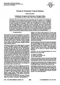
NCS take different forms, and two major types of control systems can be identified: shared-network control systems and remote control systems. The hands-on course proposal targets the first type, although several concepts can also be applied to the second type. Hence, the course context is the NCS illustrated in Figure 1.1. Several control loops, each one formed by a sensor, a controller and an actuator implemented in physically separated nodes, share a single broadcast domain to exchange the control data required for each control loop operation. In addition, other nodes, represented by the load boxes, also use the network to exchange other non-control data. For a given networked closed loop system, a control job will denote the required operations for each plant update. Hence, each control job would basically require sending the sensor reading in the sensor message after sampling the plant, and sending the control signal in the control message after computing its value in the controller node using the information contained in the incoming sensor message. Thus, in terms of bandwidth utilization, each control job simplifies to sending two messages, the sensor and the control message. The most common design and implementation approach for NCS consists in the periodic execution of the control algorithm, which implies that messages from sensors to controllers and from controllers to actuators are periodic [8]. The course will cover these methods, but will also takle other

4

actuator plant sensor

actuator plant sensor Network

controller

load

controller

Figure 1.1: Networked control system scheme approaches that go beyond the periodicity of the standard approach. Among them, two new tendencies for the analysis and design of NCS can be identified. The first one is to apply rate adaptation techniques where the period is selected according to the controlled system dynamics and/or to the bandwidth conditions, e.g. [9–11]. The main goal of these approaches is to improve the aggregated control performance for the set of control loops by efficiently using all the communication bandwidth. The second tendency is to apply event-based sampling techniques which produce non-periodic executions of the control algorithm, and therefore, non-periodic messaging in the network, e.g. [12–14]. The main goal of these approaches is to minimize the bandwidth utilization while still guaranteeing stability and acceptable control performance.

1.3 1.3.1

Experimental set-up Introduction

The desired scheme for each experimental setup is illustrated in Figure 2.3. Hence, each student (or student group) will have a two-node NCS in which one node acts as a controller (left node) while the other node acts as a sensor and actuator (right node) and is attached to the plant. The reason for putting together the sensor and actuator in the same node is to save hardware resources. The controlled plant and processing platform (hardware, real-time operating system, and network) have been carefully selected to have a friendly, flexible, and powerful experimental set-up.

1.3.2

Plant

Many standard basic and advanced controller design methods rely on the accuracy of the plant mathematical model. The more accurate the model, the more realistic the simulations, and the better the observation of the 5

Figure 1.2: Experimental setup.

Figure 1.3: Plant: electronic double integrator (DI) circuit effects of the controller on the plant. Hence, the plant was selected among those for which an accurate mathematical model could easily be derived. Following the same reasons discussed in [7], a simple electronic circuit in the form of a double integrator (Figure 1.3) was selected1 . The relative simplicity of its components together with the inherent unstable dynamics that makes the control more challenging have been the main reasons for its selection. Note however that experiments using other plants can be complementary to the approach presented here. The selection of an electronic circuit as a plant has also an important advantage: depending on the specific circuit, it can be directly plugged into a micro-controller without using intermediate electronic component. That 1

Note that in the integrator configuration, the operational amplifiers require positive and negative input voltages. Otherwise, they will quickly saturate. However, since the circuit is powered by the micro-controller, and thus no negative voltages are available, the 0V voltage (Vss ) in the non-inverting input has been shifted from GND to half of the value of Vcc (3.3V) by using a voltage divider R3 . Therefore, the operational amplifier differential input voltage can take positives or negatives values.

6

Component R3 R1 R2 C1 C2

Value 1kΩ 100kΩ 100kΩ 470nF 470nF

Table 1.1: Electronic components values is, the transistor-transistor logic (TTL) level signals provided by the microcontroller can be enough to carry out the control. Note that this is not the case, for example, for many mechanical systems. Such a simplification in terms of hardware reduces the modeling effort to study the plant and no models for actuators or sensors are required. The DI nominal electronic components are shown in table 1.1. The operational amplifier in integration configuration [15] can be model by Z t Vin − Vout = dt + Vinitial (1.1) RC 0 where Vinitial is the output voltage of the integrator at time t = 0, and ideally Vinitial = 0, and Vin and Vout are the input and output voltages of the integrator, respectively. Taking into account (1.1), and the scheme shown in Figure 1.3, the double integrator plant dynamics can be modeled by dv2 dt dv1 dt

−1 u R2 C 2 −1 v2 R1 C 1

= =

In state space form, the model is       0 R−1 v˙ 1 v1 C 1 1 = + v˙ 2 v2 0 0     v1 1 0 y = v2

0 −1 R2 C2



u

Taking into account the tolerances in the electronics components (5% for resistors and 25% for capacitors), the model that best adapts to the real plant is given by the values listed in table 1.2. 7

Component R1 R2 C1 C2

Value 100kΩ 100kΩ 420nF 420nF

Table 1.2: Validated values for the electronics components. The model validation has been performed applying a standard control algorithm with a sampling period of h = 50ms, with reference changes, and c comparing the theoretical results obtained from a Simulink model with those obtained from the plant. Hence, with the validated values for the components, the model is given by     0 −23.809524 0 x˙ = x+ u (1.2) 0 0 −23.809524   1 0 x y =

Figure 1.4 shows the results of this validation. In particular, the controller gain designed via pole placement locating the desired closed loop  poles at λ1,2 = −15 ± 20i is K = 0.5029 −0.9519 . Since the voltage input of the operational amplifier is 1.6V (which is half Vcc : the measured Vcc is 3.2V although it is powered by 3.3V), the tracked reference signal has been established to be from 1.1V to 2.1V (±0.5V around 1.6V). For the   tracking, the feedforward matrix Nx is zero and Nx = 1 0 . Note that the plant is unstable because the eigenvalues of the system matrix are λ1,2 = 0. The goal of the controller is to make the circuit output voltage (v1 in Figure 1.3) to track a reference signal by giving the appropriate voltage levels (control signals) u. Both states v1 and v2 can be read via the Analog-to-Digital-Converter (ADC) port of the micro-controller and u is applied to the plant through the Pulse-Width-Modulation (PWM) port.

1.3.3

Processing platform

The processing platform consists of the hardware platform, the real-time operating system and the network. As hardware platform, a micro-controller based architecture was selected because NCS are typically implemented using this type of hardware. As discussed in [7], for the processing platform adopting the Flex board [16] (in its full version, Figure 1.5) equipped with a R DSC micro-controller dsPIC33FJ256MC710 represents Microchip dsPIC 8

2.5 x1 x2 reference u

voltage(V)

2

1.5

1

0.5

3

3.5

4

4.5 t(s)

5

5.5

(a) Theoretical simulated plant response

2.5 x1 x2 reference u

voltage(V)

2

1.5

1

0.5 2000

2500

3000

3500 t(ms)

4000

4500

(b) Experimental plant response

Figure 1.4: Model validation.

9

6

Figure 1.5: Full Flex board. a good compromise between cost, processing power, and programming flexibility. And regarding the real-time operating system, Erika Enterprise real-time kernel [16] was selected because it provides full support to the Flex board in terms of drivers, libraries, programming facilities, and sample applications, and it gives support for preemptive and non-preemptive multitasking, and implements several scheduling algorithms [17]. In addition, its API provides support for tasks, events, alarms, resources, application modes, semaphores, and error handling, permitting to enforce real-time constraints to application tasks to show students the effects of sampling periods, delays and jitter on control performance. Regarding the network, the CAN (Controller Area Network, [18]) protocol that was originally designed for the automotive industry, but it has also become a popular bus in industrial automation as well as other applications has been selected. CAN provides the basis for many cost-effective distributed embedded applications, and its properties and functionality such as reliability, dependability, or clock synchronization, are being constantly enhanced. Once the platform is ready, the networked setup for each student looks like as in Figure 2.3 (top). The bottom board acts as a (remote) controller, and communicates via CAN with the top board, that acts as a sampler and actuator. Note that the same hardware, micro-processor based control can also be tested. In this case, the bottom board is not used, and the top board performs all the activities: sampling, control algorithm computation

10

Figure 1.6: Controller-sensor/actuator hardware (top). Details of the CAN, DI and RS232 daughter boards (bottom) and actuation. The daughter boards plugged into the top and bottom board, illustrated in Figure 1.6 (bottom), serve different objectives: the daughter board in the bottom is for CAN communication, the one in the middle is for RS232 communication (for monitoring) and the top daughter board is the DI circuit also enabled with CAN communication. It is interesting to note that the modular architecture design permits to network all the different students setups in a single CAN network. In 11

Figure 1.7: Scheme of the overall networked control system. this way, a full networked control system can be built, where several nodes acting as controllers, sensors and actuators control different double integrator systems. This richer setup will permit to observe the interaction among different closed-loops in terms of bandwidth utilization and control performance. In addition to all the pair of controller and sensor/actuator nodes that constitute several loops closed over the network, another node can be added to the network acting as a monitor/supervisor. The hardware of this node is again the full Flex board, equipped with the daughter board with CAN communication and the RS232 board used for debugging purposes. The role of this node is to gather information of the state of all the control loops, as well as to monitor and manage the network bandwidth. This node would be mainly used for the instructor/teacher, although it can be also used by students. The complete scheme showing N control loops together with the supervisor/monitor is illustrated in Figure 1.7. In the figure, each group is a pair of controller and sensor/actuator nodes that are connected using CAN (that would correspond to the setup shown in Figure 2.3 top) and it is the hardware setup for each student (or group of students). Then, all the groups can be networked between them, using also CAN, and the monitor/supervisor 12

Figure 1.8: Example of networked control system. node can also be attached to the network. Figure 1.8 shows an example of the full NCS with two groups, together with the monitor. In this case, one of the groups has the controllersensor/actuator hardware and the monitor hardware plugged together in a single tower (on the right).

1.4

Software

This section briefly describes the main software components that have been prepared for the experimental setup. Two types can be distinguished. First, the software that goes to each node (Flex board) and second, the software that can be run in an external PC for monitoring purposes, and that is called “DCSMonitor” in Figure 1.7. The node codes, the DCSMonitor, and other information related to this hands-on course are available at http: //code.google.com/p/pfc-platform-test/source/browse/. Compared to the lab proposed in [7], where the plant dynamics where monitored from Matlab, the DCSMonitor provides a set of reacher and flexible features to monitor the NCS. It has to be noted that the DCSMonitor and all the information that it monitors still can be used with the old Matlab monitoring system.

13

CPU mySystem { OS myOs { EE_OPT = "DEBUG"; CPU_DATA = PIC30 { APP_SRC = "setup.c"; APP_SRC = "e_can1.c"; APP_SRC = "code.c"; MULTI_STACK = FALSE; ICD2 = TRUE;}; MCU_DATA = PIC30 {MODEL = PIC33FJ256MC710;}; BOARD_DATA = EE_FLEX {USELEDS = TRUE;}; KERNEL_TYPE = EDF { NESTED_IRQ = TRUE; TICK_TIME = "25ns";};}; TASK TaskReferenceChange { REL_DEADLINE = "0.005s"; PRIORITY = 3; STACK = SHARED;SCHEDULE = FULL;}; TASK TaskController { REL_DEADLINE = "0.05s"; PRIORITY = 3; STACK = SHARED; SCHEDULE = FULL;}; COUNTER myCounter; ALARM AlarmReferenceChange { COUNTER = "myCounter"; ACTION = ACTIVATETASK { TASK = "TaskReferenceChange"; };}; ALARM AlarmController { COUNTER = "myCounter"; ACTION = ACTIVATETASK { TASK = "TaskController"; };}; };

Figure 1.9: Configuration file (conf.oil) for the controller node

1.4.1

Main software in NCS nodes

The description of the Erika codes is ordered according to the three type of nodes: controller, sensor/actuator, monitor/supervisor. For each node, the kernel configuration file conf.oil specifies the main parameters for the dsPIC and real-time kernel, and the code.c contains the main functionality. Controller node The configuration file is shown in Figure 1.9. It specifies the C files that are used in this node, the scheduling algorithm (EDF, Earliest Deadline First), and it defines two tasks, TaskReferenceChange and TaskController, which are implemented in the code.c and associated to an alarm to control their periodicity of execution. 14

TASK(TaskReferenceChange){ if (r == -0.5){r=0.5; LATBbits.LATB14 = 1; }else{ r=-0.5; LATBbits.LATB14 = 0;} Send_Controller_ref_message(&r); } TASK(TaskController){ x0=*(p_x0);//Get state x[0] from CAN msg //from rx_ecan1_message1[0]..[3] data field x1=*(p_x1);//Get state x[1] from CAN msg //from rx_ecan1_message1[4]..[7] data field x_hat[0]=x0-r*Nx[0]; x_hat[1]=x1-r*Nx[1]; u_ss=r*Nu; u=-k[0]*x_hat[0]-k[1]*x_hat[1]+u_ss; /* Check for saturation */ if (u>v_max/2) u=v_max/2; if (u RT-Druid Oil and C/C++ Project, enable “Create a Project” using on of these templates, and open “pic30”, open “FLEX”, and select ”EDF: Periodic task with period 0.5s”. In the first little window, click “Next”, give it a name such as ”example”, click “Next” and finally “Finish”. – Then it appears in the ”project explorer” window the “example” project with the .oil (kernel configuration file) and the .c (code file, where we have the actual program code) 49

– To compile, it must be remembered that it is always required to modify and save either the .oil or the .c. Then, to compile, go to Project − > Build Project. If everything is correct, it will appear in the terminal “Compilation terminated successfully!”. And in the ”project explorer” a new ”Debug” folder must appear, where the pic30.cof file is located, which is the binary file to be downloaded to the board using MPLAB. • Execute MPLAB

– in File − > Import: go to the workspace, and inside of the RT-Druid project just created, and inside of the Debug folder, select the .cof. – To download the file to the dsPIC, click on the second yellow icon with a down arrow. – To execute the file, click on the icon with an ascending step. – To stop it, click on the icon with a descending step.

The led should start blinking. 2. To start working with the DI circuit, the first thing to do is the open loop control. This means that it will be necessary to apply a reference signal in the form of a square wave of amplitude from 1V to 2.5V and frequency 1Hz to the plant input. This will be done using the PWM. The plant output can be read using the ADC, and the data is sent to Matlab using RS232 for better displaying the response. To do so, the following steps must be performed: • 11sdcDI.zip: this file must be unzipped in ”...\Evidence\examples\pic30”. In the new created folder, ”...\examples\pic30\11sdcDI”, 5 files can be found: – template.xml: it’s a meta-data file, that is not really used. – RS232 mfile.m: it’s the Matlab file that will get the data sent from the board through the RS232 port. It works as an ”oscilloscope”. – conf.oil: kernel configuration file. It includes details of the kernel configuration as well as the definition of the tasks that the kernel will execute. In particular it defines: ∗ TASK TaskReferenceChange: it generates the reference signal previously described ∗ TASK TaskController: it will code the control algorithm 50

∗ TASK Send: it sends data through RS232. In addition, it defines which alarms are associated to each task. Alarms will then be used in the code.c to activate the associated tasks (in the main). Their definition is as follows: ... ALARM AlarmReferenceChange { COUNTER = "myCounter"; ACTION = ACTIVATETASK { TASK = "TaskReferenceChange"; }; }; ALARM AlarmController { COUNTER = "myCounter"; ACTION = ACTIVATETASK { TASK = "TaskController"; }; }; ALARM AlarmSupervision { COUNTER = "myCounter"; ACTION = ACTIVATETASK { TASK = "TaskSupervision"; }; }; If more tasks were to be defined, they should be specified in this configuration file using the same structure. – setup.h: it includes those libraries required for the circuit control, as well as other definitions. – code.c: actual program code that includes: ∗ int main(void): main program where tasks periodicity is configured in milliseconds (with the last parameter of function SetRelAlarm) as follows SetRelAlarm(AlarmReferenceChange, 1000, 1000); // reference changes every 1000ms=1s SetRelAlarm(AlarmController, 1000, 1000); //Controller activates every 1000ms SetRelAlarm(AlarmSupervision, 1000, 10); //Data is sent to the PC every 10ms Note that the two timing constraints refer to the initial offset and the period. For example, for the SetRelAlarm(AlarmSupervision, 1000, 10), the TaskSupervision will start executing after 1s (first parameter, 1000), with a periodicity of 10ms (second parameter, 10). 51

∗ TASK(TaskReferenceChange): it generates the reference signal as follows TASK(TaskReferenceChange) { if (r == -0.5) { r=0.5; LATBbits.LATB14 = 1;//Orange led switch off }else{ r=-0.5; LATBbits.LATB14 = 0;//Orange led switch on } } ∗ void Read State(void): function that is used every time the plant output/s must be read (it reads the ADCs). ∗ TASK(TaskController): tasks that codes the control algorithm. In open loop, it has the following code TASK(TaskController) { /* sampling */ Read_State(); // returns x[0] and x[1] /* control law */ u=r; /* Check for saturation */ if (u>v_max/2) u=v_max/2; if (uv_max/2) u=v_max/2; if (uv_max/2) u=v_max/2; if (u N ew− > N ewP roject, and select Evidence− > RT − DruidOilandC/C + +P roject (figure 3.8). Next uncheck the square Use default location, and we must go to search the Sensor code in this folder : /home/student/workspace/P rograms/DSP ICS EN SOR/trunk An then lets put a name to the project (figure 3.9). Once we have the new project we can compile it clicking in P roject− > Clean, with this action we will clean the foulder firstly, and check the option Start build immediately to compile the code before we clean the folder (figure 3.10). 70

Figure 3.5: Live CD desktop.

Figure 3.6: Laboratory programs compressed code.

Figure 3.7: Eclipse working directory.

71

DCSMonitor

DSPIC SENSOR

DSPIC CONTROLLER

DSPIC MONITOR

This is the program that runs on your computer to see the control. You need to communicate via RS232 with a FLEX board with program dsPIC SENSOR installed. This program is for one FLEX board and it will modify the values of the double integrator and read his output value. The device programmed with this code is named Sensor/Actuator. Because it reads the output value of the integrator (this is the task of a Sensor) and writes the input value to the DI (this is a task of a Actuator). This program is for one FLEX board and calculates the control value for the DI and send it to the actuator using the CAN bus. This program is for another FLEX board, and it can monitory all the CAN bus.

Table 3.3: Files in ∼ /workspace/P rograms/

Figure 3.8: Creating a new RT-Druid project in Eclipse. It will starts to compile and before this in the text box at bottom of the

72

Figure 3.9: Selecting project folder in Eclipse. program we will see the message: Compilation terminated successfully!

3.3.3

Programming DSPIC SENSOR with MplabX

Once we compiled the program, let’s open MplabX program (figure 3.11) We will create a new project importing an .elf file generated by Eclipse: F ile− > ImportHex(P rebuilt)P roject Then we must search the file generated with Eclipse (figure 3.12): /home/student/workspace/Programs/DSPIC SENSOR/trunk/Debug/pic30.elf Next step is to select the device to be programmed (figure 3.13), in our case is : • Family: DSPIC33 • Device: dsPIC33FJ256MC710 Now is time to select which programmer we want to use, in our case we use the mplab ICD3 programmer to program the FLEX boards (figure 73

Figure 3.10: Cleaning and compiling in Eclipse.

Figure 3.11: MplabX loading logo. 3.15). In this moment we must connect the programmer mplab ICD3 to the FLEX board to be programmed (figure 3.14): In case of select another programmer we need to know what the colour means, look into the next table 4.1. At last we only have to select a name for this project (figure 3.16), and it is very important to change the directory out of Debug (figure 3.17). If

74

Figure 3.12: Selecting pre-compiled file in MplabX.

Figure 3.13: Selecting device in MplabX.

Figure 3.14: Mplab ICD3 and FLEX board connected. we leave this by default when we modify the source code with Eclipse and make a Clean we would have problems with this project in MplabX. Finally MplabX will show up all details of this new project, so we accept and would have all the environment prepared to program the microcontroller. To program the FLEX board, we must click at button Make and Program Device up to the right , once MplabX programmed the device will show this message (figure 3.18).

75

Figure 3.15: Choosing programmer in MplabX. Green Yellow

Red

This colour means that the programmer is fully functional in this version. . This colour means that the programmer is partially functional in this version. In this case it is possible to select, but it may not work. This colour means that the programmer is not functional in this version. In this case is not possible to select it. Table 3.4: Programmers compatibility in MplabX

Figure 3.16: Selecting the name of the project in MplabX.

Figure 3.17: Location of the project in MplabX.

3.3.4

Summary to program the other devices

The steps to compile and program the other devices (whith DSPIC CONTROLLER and/or DSPIC MONITOR) are the same that we did to program the DSPIC SENSOR. 76

Figure 3.18: Microcontroller programmed correctly in MplabX. This section is a summary of all steps to program any device: 1. Decompress codes needed from /home/student/workspace/P rograms/ 2. Open the Eclipse program (a) Create a new RT-Druid project (b) Select the folder where the project is, and we must put a name to the project. (c) We must to create the project (d) Clean and compile 3. Open MplabX program (a) Create a new project with the pre-compiled code generated by Eclipse (b) Search the file .elf (in the project folder into Debug) (c) We must select the microcontroller DSPIC33 and dsPIC33FJ256MC710 (d) Connect the ICD3 to the computer and the FLEX board (e) Select the ICD3 programmer serial number (f) Put a name to the project and delete the Debug part of the location (g) Accept and program

77

3.3.5

DCSMonitor

DCSMonitor is a program used to see the control being executed in one plant. To execute this program you must go to desktop and click in DCSMonitor (figure 3.19).

Figure 3.19: Directory with DCSMonitor code. Once we opened the program we will see this window 3.20. In this program we can view our control in a graph at middle left of the window. To the right there is a button to connect to serial port. Just below if we are connected to a Monitor device we will see all plants in the CAN bus. And below of this you can select which plots you want to see. Then there is a button to start receiving data of a plant, and another to clean the text. Finally we can see statistical values. Firstly we need to specify in preferences which device we want to connect, and we can choose the language (figure 3.21). Once we have selected the language and which device we want to connect we would push connect button, if it is fine we would see connected in green color 3.22. Then if we are connected to a Monitor device go to section 3.3.5. Otherwise if you are connected to a Sensor/Actuator device go to section 3.3.5. Connected to Sensor/Actuador device In this execution mode is only enabled monitoring option, clean text and graphic export, so you may start clicking monitor button, and if you have the Sensor/Actuator connected to serial port we would see the real time graph. And in the text box we would see all received data. Like the figure 3.23. If we want to export the graph firstly we need to stop the monitoring (see the section 3.3.5).

78

Figure 3.20: DCSMonitor main window.

Figure 3.21: Preferences. Connected to Monitor device In this execution mode we have all the options enabled. Firstly we must click the buttonbList devices and then we would see a list with all id plants connected to CAN bus (there is an example 3.24). Once we had a list of plants, it is recommended to stop updating devices list, because computer and Monitor device will work faster. 79

Figure 3.22: DCSMonitor connecting to serial port.

Figure 3.23: DCSMonitor program connected to a Sensor/Actuador device when we are monitoring we would see a real time graphic and data in the text box. After that we must select any id plant of the list and click in Monitorize button to start receiving his values. Then we would see a real time graphic and their values in text box below (figure 3.25). We can enable or disable 80

Figure 3.24: Requesting for id plants in the CAN bus to DCSMonitor device. any of the plots checking it in the options section at the right (figure 3.26).

Figure 3.25: All plots in the graphic. There is an other option in this execution mode, we can send a message to the Monitor device to start sending messages into CAN bus, it is possible dragging the Saturation bar (figure 3.27) since the wanted value. This will 81

Figure 3.26: Only reference and second integral in the graph. provoke monitor device to send maximal prioriti messages into the CAN bus.

Figure 3.27: Saturation bar.

Graph exporting In all execution modes we can take an instance of the graph. To do that we must stop the monitoring in the wanted instance, then check the plots to be showed in the Options panel, and finally push the button Export graph figure 3.28). You only need to select the folder and assign a name to the file, with preferred extension (.pdf, .eps, .ps, .png, and more) (there is an example exporting an image to the desktop in figure 3.29).

82

Figure 3.28: Choosing a name for the exported graph.

Figure 3.29: Example of exported graphic.

3.4

Installing

It is possible to install this Live CD into the computer side by side with another Operating System or alone. You must know that installing an op83

erating system may erase your important data, so you must make this at your own risk. There is also the option to create a virtual machine (with VirtualBox or VMWare program) and thus work from our current operating system, and running a virtual machine with the laboratory. Then you can see a step by step guide on how to install the live CD. In the Live CD main menu (figure 3.30), select the option Install.

Figure 3.30: Live CD main menu, installing on computer. Once we selected install we will see Ubuntu logo (figure 3.31) and then the CD will prepare the installation environment.

Figure 3.31: Ubuntu loading log. Once the environment is ready, then we may choose the language, and after that click on next. Then select your time zone to synchronise the computers time. And after that select your keyboard distribution. At this point we need to choose where install the Live CD (figure 3.32). The options are: • Install LiveCD next to other operating system (recommended option) • Install LiveCD in the entire disc. • Install LiveCD partitioning the disc manually (advanced).

84

Figure 3.32: Hard disc partitioning. If we don’t know wich option choose, we must select the first option. Once we finish this step, we would see an advertisement indicating the disc modifications. This step is not reversible, then accept in our own risk. Now we must wait until it finish partitioning. Once the disc is parted we must select an user and password (figure 3.33). This LiveCD was created to be the user and password student then you need to specify this string. Once we specified all the options, we would see a summary. When we accept this it will start installing the system (this may take some time depending on the machine). When the bar get the 100% we will see an advertisement of completed installation, then click on reboot now, extract the disc and push enter. When the computer starts we must select the new operating system Ubuntu. And then introduce the user and password student (figure 3.34). Now we will have the environment ready to try the differents device programs (LiveCD desktop 3.35). If the LiveCD is installed in a VirtualBox we can install the package Guest Additions. This package will give us a lot of facilities to interact with the virtual machine. To install this package you must start the virtual machine, once you will in the desktop select the option in the window Devices− > InstallGuestAdditions, this action will create a new virtual disc in your virtual desktop, then you 85

Figure 3.33: User and password configuration: we must specifiy user and password student.

Figure 3.34: Login. must open it and follow his instructions. There is a known problem if your host is an Ubuntu machine, after you installed the Guest Additions it is possible that it do not work properly. Then in the virtual machine you must do this steps in a terminal: 1. sudo apt-get update 2. sudo apt-get install build-essential linux-headers-$uname − r 86

Figure 3.35: Live CD desktop in new installation 3. sudo apt-get install virtualbox-ose-guest-x11

87

Chapter 4

Quick guide to start working 4.1

Development Environment

To program the Flex boards for conducting laboratory you need to have development environment ready with the following programs: • Eclipse (EE 160) : programming environment, renamed Erika Enterprise (EE) RTDruid. • Mplab (mplabx ide beta 7) : program to burn binaries to dsPIC. • Matlab (matlab 7.8) : program to establish communication between computer and dsPIC. • Python (Python 2.7) : python shell. – PySerial : Serial communication package. – Matplotlib : Package to draw graphic plots. All this programs are free of charge (Matlab is an exception), and all of this can be downloaded in his official web-pages: • Eclipse

http://erika.tuxfamily.org/erika-for-multiple-devices.html

• Mplabx

http://ww1.microchip.com/downloads/mplab/X_Beta/installer. html

88

• Python

http://www.python.org/download/

• PySerial

http://pypi.python.org/pypi/pyserial

• Matplotlib

http://matplotlib.sourceforge.net/users/installing.html

• PyQT4

http://www.riverbankcomputing.co.uk/software/pyqt/download

Python packages sudo apt-get install gnuplot sudo apt-get install pythonmatplotlib sudo apt-get install python-scitools sudo apt-get install pythonqt4

4.1.1

Mplab installation

MplabX needs Java to be run, in most cases (in our case running Ubuntu) this is pre-installed, but in other cases it is necessari to download and install from his official web-page: http://www.java.com/es/ If you need to install it in Ubuntu, you can do it directly from terminal with the next commands: sudo apt-get update sudo apt-get install default-jre Once Java is installed, go to MplabX web-page (figure 4.1) and select : • MPLAB IDE X Beta • MPLAB C30 Lite Compiler for dsPIC DSCs and PIC24 MCUs http://ww1.microchip.com/downloads/mplab/X_Beta/installer.html Once downloaded, open a terminal to install them (Figura 4.2): Access the directory where the files have been downloaded and verify that indeed have been downloaded: cd ~/Downloads/ ls 89

Figure 4.1: MplabX Official page. In this page you can download last version of this program.

Figure 4.2: Opening a terminal: to open a terminal go to Applications -¿ Accessories -¿ Terminal.

Figure 4.3: Installing MplabX IDE We give permission to run mplabx-ide and install MplabX IDE (Figura 4.3): chmod u+x mplabx-ide-beta7.12-linux-installer.run sudo ./mplabx-ide-beta7.12-linux-installer.run 90

Then we’ll just accept all the conditions of use (Figura 4.4) and specify the installation directory (Figura 4.5), we can let this by default to ‘/opt/microchip/mplabx‘.

Figure 4.4: Use conditions on MplabX IDE: we need to accept this terms and conditions of MplabX

Figure 4.5: MplabX installation directory: we can let this by default After that we need to reboot (Figura 4.6), but firstly install the other 91

package.

Figure 4.6: MplabX IDE installations end: it says that we need to reboot. Once we have installed MplabX IDE, lets go to install the other package: chmod u+x mplabc30-v3.30c-linux-installer.run sudo ./mplabc30-v3.30c-linux-installer.run Likely the other installation we need to accept terms and conditions (Figura 4.7) and let installation directory by default to ‘/opt/microchip/mplabc30/v3.30c‘

Figure 4.7: MplabX C30 compiler’s terms: we accept this terms.

92

Figure 4.8: MplabX C30 compiler’s installation directory: it is recommended to let by default.

4.1.2

Eclipse installation

Here we are going to install Eclipse following the steps of his web-page: http://www.eclipse.org/ There is in Linux repositories. Lets do this in a terminal: sudo apt-get update sudo apt-get upgrade sudo apt-get install eclipse

4.1.3

Installing RTDruid plugin on Eclipse

Once we installed Eclipse, we need this plugin to program the RTOS Erika. Lets do this steps: Go to: • Help -¿ Install new Software... We need to add a new entry (Figura 4.10) clicking in: • Add... In next window (Figura 4.11) fill entries with next data: • Name ->RTDruid 93

Figure 4.9: Installing Eclipse’s plugin: to install new plugins in Eclipse go to Help -¿ Install new Software...

Figure 4.10: Window to add new plugins: in this window we can add new Eclipse’s plugins. • Location ->http://download.tuxfamily.org/erika/webdownload/ rtdruid_160_nb/ Then it must be to appear the packages that there is in this url (Figura 4.12), we need to check all of them. Then will appear a summary of the packages to be installed, lets accept terms and conditions (Figura 4.13) Be aware on installation because there is a moment that will popup a hidden advisement about the trust of the package, and we need to accept it (Figure 4.14). Finally we must to reboot the computer for the changes to take effect. 94

Figure 4.11: Adding new plugin’s url: here we can add urls to Eclipse’s plugins.

Figure 4.12: Available plugins: there is a list of plugins available in the url. Then reboot it (Figure 4.15). It is necessary to specify the path of the compiler to RT-Druid to compile and generate .elf files. Then specify this going to: 95

Figure 4.13: RTDruid terms and conditions: we need to accept this.

Figure 4.14: Trust of the package RTDruid: we need to accept the trust of RTDruid. • Window -> Preferences In the preferences go to: 96

Figure 4.15: Reboot Eclipse: we need to reboot Eclipse. • RTDruid -> Oil -> dsPic And we must check if the path is correct (Figure 4.16) (Be careful because its possible that you have another Mplab version, but this is an example of how it must to seem: • Gcc path /opt/microchip/mplabc30/X.XXy • Asm path /opt/microchip/mplabx/asm30

Figure 4.16: RTDruid compilator’s path: here we must introduce the path of MplabX installation. With this steps we will have the environment to program the microcontrolers with the Real-Time Operating Systems Erika 97

4.2

Led Blinking

Here we can see the necessary steps to create a new project with a template, and then compile and program the microcontroler.

4.2.1

Eclipse environment

Firstly we need to open Eclipse, this is an programming IDE, and in this case we will use the RTDruid plugin of Evidence. This plugin will allow to program RTOS Erika. Once the program is opened, lets create a new project (Figure 4.17) • File -> New -> Project...

Figure 4.17: RTDruid new project. We must to select this kind of project (Figura 4.18): • Evidence -> RTDruid Oil and C/C++ Project

98

Figure 4.18: Selecting type of RTDruid project. Then we must assign a name to this project (Figura 4.19) and let the other options by default (you could change the directory, but we recommend to let by default to workspace). In this step we can select a template for the project (Figura 4.20), this will give us all the basic structure to program Erika RTOS. So lets do the following steps: Check the box Create a project using one of these templates and select pic30 (because in this case we want to program a dsPIC33) and here select any of this templates templates, in our case: • pic30 -> FLEX -> EDF: Periodic task with period Once we push the Finish button we will have all the environment ready to compile de program. In case of option Build Automatically is activated, Eclipse will compile automatically the first time. It is needed to deactivate this option now. So lets check if the option Build Automatically” is unchecked (Figure 4.22): • Project -> Build Automatically 99

Figure 4.19: Assigning name to a RTDruid new project.

Figure 4.20: Templates RTDruid: in this section we may select any of this templates. This only need to be compiled and programmed to the FLEX board.

100

Figure 4.21: Eclipse environment: ready to compile.

Figure 4.22: Eclipse environment: build In this moment we can modify the code. When we want to compile the code we could firstly save the project (if you do not save the project before compiling, the code compiled may not be the last), once we saved the project go to: • Project -> Clean We want to clean to be sure that compiled code is the last saved, and let the other options by default (Figure 4.23) (this options will clean the project and compile it), or select Clean projects selected below and Build only the selected projects to clean and compile only the selected project.

101

Figure 4.23: Compiling in Eclipse: before compile it is recommended to clean the project. Once the compilation is complete it will show this message Compilation terminated successfully! (Figure 4.24), in this step we would have a new pic30.elf file in Debug directory. This is the file to be saved in the microcontroller with MplabX.

Figure 4.24: Eclipse compiled successfully message. It is possible that in the compilation step RTDruid do not find compilator’s path. In this case check you would check if the installation step 4.1.3 is correct (Figure 4.16).

102

4.2.2

Mplab X environment

Once we have created the pic30.elf file, is time to open the program MplabX. With this program we would program the microcontroller. Then lets open the program, and lets to create a new project (Figure 4.25): • File -> New Project...

Figure 4.25: MplabX new project. Now the program let us to choose the project kind. In our case we have precompiled file and then we want to select our file (Figure 4.26).

Figure 4.26: MplabX precompiled project. • Categories : Microchip Embedded • Projects: Prebuilt (Hex, Loadable image) Project 103

In next section we need to select our precompiled file, so lets select it (Figure 4.27). If you done all this guide steps, the path must be like this: • home/student/workspace/f lexb link/Debug/pic30.elf

Figure 4.27: Selecting precompiled file in MplabX. In this step we need to select witch microcontroller we want to program (Figura 4.28), in our case it is:

Figure 4.28: Selecting device in MplabX. • Family: DSPIC33 104

• Device: dsPIC33FJ256MC710 Now is the time to select the programmer, in our case to program the FLEX boards we need the Mplab ICD3 programmer (Figura 4.30). We need to connect the programer to the FLEX board in this moment (Figura 4.29):

Figure 4.29: Flex and Mplab ICD3: ready to be programed.. In case of choose another programmer, we need to know what means the the colour in the list:

Figure 4.30: List of programmers in MplabX: the colours of the programmers have a meaning that can be consulted at table 4.1. At last we only have to select a name for this project (Figure 4.31), and it is very important to change the directory out of Debug (Figure 4.32). If 105

Green Yellow

Red

This colour means that the programmer is fully functional in this version. . This colour means that the programmer is partially functional in this version. In this case it is possible to select, but it may not work. This colour means that the programmer is not functional in this version. In this case is not possible to select it. Table 4.1: Programmers compatibility in MplabX

we leave this by default when we modify the source code with Eclipse and make a Clean we would have problems with this project in MplabX.

Figure 4.31: Selecting a name for the project in MplabX.

Figure 4.32: Taking out of the directory Debug: if we leave this by default when we modify the source code with Eclipse and make a Clean we would have problems with this project in MplabX. Finally MplabX will show up all details of this new project, so we accept and would have all the environment prepared to program the microcontroller. To program the FLEX board, we must click at button Make and Program Device up to the right (Figura 4.33). Once we have programmed the board, the first orange led of the left would start blinking (Figura 4.34). 106

Figure 4.33: Programming FLEX board with MplabX: to program any controller we need to click this button.

Figure 4.34: FLEX board running program Blink : with this program the first led will blink every half second.

107