Design of a Path-Tracking Steering Controller for Autonomous Vehicles

Article

Design of a Path-Tracking Steering Controller for Autonomous Vehicles Chuanyang Sun 1, Xin Zhang 1,*, Lihe Xi 1 and Ying Tian 2 School of Mechanical, Electronic and Control Engineering, Beijing Jiaotong University, Beijing 100044, China; [email protected] (C.S.); [email protected] (L.X.) 2 Beijing Jiaotong University Yangtze River Delta Research Institute, Zhenjiang 212009, China; [email protected] * Correspondence: [email protected]; Tel.: +86-010-5168-8404 1

Received: 25 April 2018; Accepted: 1 June 2018; Published: 4 June 2018

Abstract: This paper presents a linearization method for the vehicle and tire models under the model predictive control (MPC) scheme, and proposes a linear model-based MPC path-tracking steering controller for autonomous vehicles. The steering controller is designed to minimize lateral path-tracking deviation at high speeds. The vehicle model is linearized by a sequence of supposed steering angles, which are obtained by assuming the vehicle can reach the desired path at the end of the MPC prediction horizon and stay in a steady-state condition. The lateral force of the front tire is directly used as the control input of the model, and the rear tire’s lateral force is linearized by an equivalent cornering stiffness. The course-direction deviation, which is the angle between the velocity vector and the path heading, is chosen as a control reference state. The linearization model is validated through the simulation, and the results show high prediction accuracy even in regions of large steering angle. This steering controller is tested through simulations on the CarSimSimulink platform (R2013b, MathWorks, Natick, MA, USA), showing the improved performance of the present controller at high speeds. Keywords: autonomous vehicles; model linearization; path tracking; steering controller; model predictive control

1. Introduction Autonomous vehicle technology aims to increase driving safety, reduce traffic congestion and emissions, and improve energy efficiency [1,2]. The ability to track the desired path accurately and steadily plays a critical role in the control task of an autonomous vehicle, especially when operating at high speeds. Therefore, a great deal of research has been done on steering control of autonomous vehicles. Full vehicle models and nonlinear tire models are usually used to simulate the vehicle response during high speeds and large-steering-angle driving [3]. However, the nonlinearity of vehicle and tire models leads to a high computational burden [4]. A bicycle model with a small-angle assumption and a proportional linear tire model are widely used in path-tracking research [5,6]. However, when the steering angle and lateral slip angle are larger than 5°, the model becomes inaccurate, especially in the region of tire-force saturation. Erlien et al. [7] introduced an affine approximation linearization method to handle the nonlinearity of the tires in the model predictive control (MPC) scheme, however, this approach is inaccurate when the length of the prediction horizon is larger. Talvala et al. [8] proposed a tire slip angle-related parameter to capture the nonlinearity even when the tire is saturated. In general, tuning the parameters of a given model to realistic values can be challenging work. Energies 2018, 11, 1451; doi:10.3390/en11061451

www.mdpi.com/journal/energies

Energies 2018, 11, 1451

2 of 18

Heading deviation and lateral deviation are usually chosen as the control reference states, and multiple approaches are presented to eliminate them [9–11]. Brown et al. [5] presented a pathtracking controller, based on an MPC with different prediction horizons, which achieved stabilization and obstacle avoidance simultaneously. Kritayakirana et al. [6] used the center of percussion as a reference point for calculating the steering command, in order to minimize both the heading and lateral deviations. Their algorithm has lower complexity and can maintain stability even when the rear tires are saturated. Katriniok et al. [12] proposed a combined longitudinal and lateral optimal control algorithm for the collision-avoidance system. The robustness of their algorithm is demonstrated through experiment. While there has been some success in these studies, choosing the heading deviation as a reference state may not effectively minimize the lateral deviation, especially when operating at high speeds. Mammar et al. [13] utilized the yaw-rate error instead of the path-tracking error as the feedback input to minimize the deviation from the path, and good robustness was demonstrated through their tests. Tagne et al. [14] presented an adaptive controller and used the steady-state sideslip and yaw rate to help bring the operating point to the desired equilibrium quickly. However, their controller is not capable of accurate path tracking in the tire-friction limit. Kapania et al. [15] pointed out that lateral deviations would be minimized when vehicle sideslip was tangential to the path, and hence designed a feedback controller to keep the vehicle velocity vector at the desired heading. However, a fixed look-ahead distance is not always optimal over a range of vehicle speeds. The capability to systematically include system constraints and future predictions in the design procedure makes model predictive control (MPC) an attractive method in the control of autonomous vehicles, where vehicle stability constraints, as well as changing vehicle and tire dynamics, exist in the system [16–19]. While MPC seems promising, when combined with the nonlinear plant model, it still faces convergence and high online computational complexity issues, making it unsuitable under high-speed conditions. On the contrary, the unique global minimum of the linear MPC can be efficiently calculated by various methods in a limited number of iterations [20,21]. Several methods that combine MPC with a linear model were proposed in References [5,7,17]. Raffo et al. [18] presented an MPC path-tracking controller with a linear kinematic model to achieve the desired performance during high-speed driving. Beal et al. [19] combined an MPC with linear vehicle and tire dynamic models to stabilize the vehicle at the limits of handling. In this paper, a methodology is proposed to allow one to linearize the nonlinearities of the vehicle and tire models under the MPC scheme, with some additional assumptions. A linear-model MPC path-tracking steering controller, using the direction deviation between the vehicle’s velocity vector and the path heading as the control reference state, is designed. Basic information about the MPC scheme is introduced in Section 2. The linearization method for the models and the simulation method for validating our approach are presented in Section 3. In Section 4, the use of different control reference states is discussed and the control objective is determined. Additionally, our proposed MPC controller is presented, including the constraints and the optimization problem. In Section 5, the simulation results verify the efficacy of the presented controller under high speeds and large lateral-acceleration conditions. Finally, Section 6 concludes the paper with a brief discussion of the results. 2. MPC Algorithms Before constructing the linearization method of the vehicle model using the prediction information, we first briefly introduce the MPC control scheme. The system to be controlled is described with a difference equation: x + = f ( x , u) ,

(1)

where x , x + and u are the state, successor state, and control input of the system, respectively, subject to the constraints:

x

, u

,

(2)

Energies 2018, 11, 1451

3 of 18

 m is a compact, convex set. We employ x( k ) and  n is a closed, convex set and u( k ) to denote the state and the control action at sampling time k. In the MPC scheme, the future behavior of the system can be predicted using the plant model f () . The control objective is to steer the state trajectory, x u () , to the desired state, xr , over a finite

where

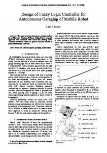
prediction horizon, NP , by applying the control sequence, u() , to the system. Figure 1 shows an example control process of the MPC.

past

xr

future

x u ()

  Δu( k + i )  u()

u( k ) x( k )

k −1

k

k + NC

k +1

k + N P time

Figure 1. Control process of the model predictive control (MPC) algorithm.

We consider the typical cost function, J NC , NP (, ) , as defined by: J NC , NP ( x u (), Δu()) =

N P −1

 ( x( k + i) − x ( k + i))

T

r

i =0

Q( x( k + i ) − x r ( k + i )) +

NC −1

 Δu( k + i ) i =0

T

RΔu( k + i ) ,

(3)

where Δu() = {Δu( k), Δu( k + 1),, Δu( k + NC − 1)} is the sequence of control input increments,

x u () = { x( k + 1), x( k + 2), , x( k + NP )} , NC is the control horizon, with the constraint NC  NP , and Q and R are the weighting matrices. At each sampling time k, MPC solves the following optimization problem:

min J NC , NP ( x( k), u( k − 1), Δu()) ,

(4)

Δu ( ), x u ( )

s.t. x( k + i + 1) = f ( x( k + i), u( k + i)), i = 0, i

u( k + i) = u( k − 1) +  Δu( k + j), i = 0, j =0

u( k + i) = u( k + NC −1), i = NC ,

Δu( k + i)  Δ , i = 0, u( k + i)  , i = 0,

x( k + i)  , i = 1,

, NP − 1 , , NC − 1 ,

, NP −1 ,

, NC − 1 ,

(5)

(6)

(7) (8)

, NC − 1 ,

(9)

, NP .

(10)

The optimal solution denoted by Δu () of Equations (4)–(10) is generated, and the control input is, therefore, defined by:

u( k) = u( k −1) + Δu ( k) .

(11)

Energies 2018, 11, 1451

4 of 18

Hence, the control u( k ) is applied to the system at time k. At the next sampling time, the optimization problem in Equations (4)–(10) is resolved over the shifted prediction horizon, and the process is thus repeated for every sampling time. Solving the optimization problem of Equations (4)–(10) is a computationally demanding task. Furthermore, the system order, control horizon length NC , and nonlinearities in the plant model f () are the main factors in determining the computational burden [22]. Usually, adequately

lowering the system order and successively linearizing the process model to formulate a linear– quadratic optimization problem are efficient ways to improve computational efficiency. 3. Modelling 3.1. Nonlinear Model 3.1.1. Vehicle Dynamic Model The single-track ‘bicycle’ model, shown in Figure 2 with two speed states and three position states, can adequately capture the tracking performance and handling stability under various operating conditions. In this scheme, the front steering angle δ is the only actuation. To make the optimization problem of δ convex, longitudinal speed Ux is not allowed to be variable. While an external speed controller could be used to track a desired speed profile, the speed over the prediction horizon is assumed to be fixed when building the process model. αf δ

r

U

Uy β

αr Δψ

b

Ux

Δ

Fyf

a

O e

Fyr

PATH HEADING

s

Figure 2. Bicycle model schematic. O is the center of mass; U and U y are vehicle speed and the lateral speed at the center of gravity, respectively.

The sideslip β and yaw rate r are described by the equations of motion [23]: β=

r=

Fyf cos(δ) + Fyr mU x

−r,

aFyf cos(δ) − bFyr I zz

,

(12)

(13)

where m and Izz are the vehicle mass and yaw inertia, respectively; Fy[f,r] denotes the lateral tire force of the front and rear axle, respectively; and a and b are the distances from the center of mass O to the front and rear axles, respectively. 3.1.2. Tire Model The lateral tire force is modelled using the Fiala brush tire model [24]; Fy[ f ,r ] = ftire (α , Fz ) , where:

Energies 2018, 11, 1451

5 of 18

  3μFz Cα2 Cα3 tan α tan α − tan 3 α, α  arctan  −Cα tan α + 2 2 ftire (α , Fz )=  3μFz 27μ Fz  Cα  otherwise −μFz sgn α,

  .

(14)

In Equation (14), μ is the coefficient of friction, Fz is the normal force, and Cα is the tire cornering stiffness. The tire slip angles αf and αr, using small-angle approximations, can be expressed as:

αf = β +

ar −δ , Ux

(15)

br , Ux

(16)

αr = β −

where δ is the front steer angle. In order to simplify the nonlinear relationship between the actuation δ and the vehicle dynamic states while taking the saturation of the tire into account, the front lateral force Fyf is considered as the control input of the model. The desired Fyf, generated by the MPC optimization, is then mapped to δ by:

δ = β+

ar −1 − f tire ( Fyf ) , Ux

(17)

−1 ( Fyf ) is the inverted tire model, which calculates the tire slip from the tire force via where f tire

numerical methods. 3.1.3. Path-Tracking Model The path-tracking model is shown in Figure 2, and the vehicle’s relative position to the desired path can be determined by three state parameters: the lateral deviation e, the heading deviation Δψ, and the distance s along the path. The path tracking model can be written as [5]:

Δψ=r − Ux κ( s) ,

(18)

e=Ux sin(Δψ) + Uy cos(Δψ) ,

(19)

s = Ux cos(Δψ) − Uy sin(Δψ) ,

(20)

where κ(s) is the curvature of the desired path at s. 3.2. Model Linearization 3.2.1. Vehicle Dynamic Model The most popular linearization method is the small-angle assumption (when δ  5 , cos(δ)  1 ). The nonlinear model of Equations (12) and (13) can thus be expressed as: β

r

Fyf + Fyr mU x

−r ,

aFyf − bFyr I zz

.

(21)

(22)

However, when the vehicle tracks a path with high curvature, the steering angle can be very large, and the small-angle assumption is invalid. The model in Equations (21) and (22) will fail to simulate the vehicle response at these operational conditions.

Energies 2018, 11, 1451

6 of 18

Consider the following suppositions: (1) Suppose the steering angle increments are fixed at every step over the prediction horizon, and are independent of the control sequence u() , that is:

δa ( k + i) = δNP , i = 0, where

, NP −1 ,

δa ( k + i) is the supposed steering angle increment at step i+1 and δNP

(23) is the

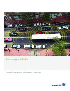
corresponding fixed increment, which will be determined later. (2) Suppose the vehicle will reach the desired path at step NP of the prediction horizon, and will subsequently track the path without deviation, as shown in Figure 3. Then, the vehicle at step NP is assumed to be in the steady state. Hence:

ea ( k + NP ) = 0 ,

(24)

δa ( k + NP −1) = δss ( k + NP − 1) ,

(25)

α[f,r],a ( k + NP − 1) = α[f,r],ss ( k + NP − 1) ,

(26)

where ea , δa and α[f,r],a are the supposed lateral deviation, steering angle, and tire slip angle, respectively, and δss , α[f,r],ss are the steady-state steering angle and tire slip angle, respectively.

αf,ss

R( k + N P − 1)

δss

βss

αr,ss

P( k + N P − 1)

R( k )

αf

PATH

δ

β

αr

P( k + 1) kk +1

k + Np − 1

Figure 3. The supposed path over the prediction horizon for the linearized model. R(k + i) and P(k + i) denote the radius of the desired path and the supposed point at s(k + i), respectively, i = 0, …, 𝑁P − 1.

Under steady-state cornering conditions, setting r = 0 in Equation (19), the front and rear tire forces are yielded:

Fyfss =

mb 2 U κ, 2L x

(27)

Fyrss =

ma 2 U κ. 2L x

(28)

Hence, the steady-state steering angle relates to the front and rear lateral tire slip by vehicle kinematics via:

δss = Lκ − αf,ss + αr,ss ,

(29)

Energies 2018, 11, 1451

7 of 18

where L = a + b is the wheel base, and αf,ss and αr,ss can be calculated from Equations (14) and (27) −1 ( Fy[ f ,r ] ) . and (28) by the inverted tire model ftire

Under the suppositions above, the supposed steering-angle increment can be written as: δa ( k + i) =

δ( k) − δa ( k + Np − 1) Np

, i = 0,

, NP −1 .

(30)

Finally, considering the slew-rate capabilities of the vehicle, the supposed steering-angle increment is determined via:  δ , δ a  δmax , δNP =  a  sign(δ)  δmax , else

(31)

and the supposed steering angle for every step of the prediction horizon is thus:

δa ( k + i) = δ( k) + i  δNP , i = 0,

, NP −1 .

(32)

Combining Equation (32) with Equations (12) and (13) yields a linearized version of our nonlinear vehicle model: β( k + i) =

Fyf ( k + i)  cos(δa ( k + i)) + Fyr ( k + i) mUx

r( k + i ) =

− r( k + i) , i = 0,

aFyf ( k + i)  cos(δa ( k + i)) − bFyr ( k + i) I zz

, i = 0,

, NP −1 ,

, NP −1 .

(33)

(34)

3.2.2. Tire Model The front lateral force is considered as the control input, and the nonlinear dynamics of the reartire force should be properly accounted for to accurately approximate the MPC with a linear optimization problem. Inspired by Reference [7], which assumes that the tire-cornering stiffness keeps constant in the prediction horizon, we propose a new online successive linearization method by combining both the information of time k and step NP of the prediction horizon to accurately

Tire Lateral Force Fyr

predict the propagation of lateral tire forces, as shown in Figure 4.

Fr ,ss Fr αr ,ss

αr

Cr

Brush model Linear approx Tire-slip angle  r

Figure 4. Linear approximation of the brush tire model. αr and αr,ss are the tire slip angle at time k and steady-state tire slip angle at step NP of the prediction horizon, respectively. Fr

and Fr,ss are

the corresponding lateral forces.

In the linearized model, the equivalent cornering stiffness over the prediction horizon is:

Energies 2018, 11, 1451

8 of 18

Cr =

( Fr,ss − Fr ) αr,ss − αr

.

(35)

Thus, the approximate expression for the predicted rear-tire lateral force is:

Fyr ( k + i) = Fr − Cr (αr ( k + i) − αr ) , i = 0,

, NP −1 ,

(36)

where αr ( k + i) is the predicted rear-tire slip angle which can be calculated by Equation (16). The resulting linear expressions for the motion equations are described as follows:   b  r( k + i ) Fyf ( k + i )  cos(δa ( k + i)) +  Fr − Cr ( β( k + i) − − αr )  U  x  − r( k + i ) , i = 0, β( k + i ) = mU x   b  r( k + i ) aFyf ( k + i )  cos(δa ( k + i )) − b  Fr − C r ( β( k + i) − − αr )  U  x  , i = 0, r( k + i ) = I zz

, NP −1 ,

, NP −1 .

(37)

(38)

3.2.3. Tracking Model Making the small-angle approximation for β and Δψ yields:

Δψ( k + i)=r( k + i) − Ux κ( k + i) , i = 0,

, NP −1 ,

(39)

e( k + i)=Ux ( β( k + i) + Δψ( k + i)) , i = 0,

, NP −1 ,

(40)

s(k + i)=Ux , i = 0,

, NP −1 .

(41)

Due to the assumption that the speed is fixed over the prediction horizon, the distance along the path can be given, a priori, as: i

s( k + i )=s( k ) +  U x , i = 1, j =0

, NP .

(42)

4. MPC Controller Design 4.1. Problem Statement Unlike human driving, which cannot perceive the velocity direction of the vehicle, autonomous vehicles can obtain more accurate information from sensors and estimation technology. Taking the heading deviation Δψ as a control reference state does not maximize the capacity of an autonomous vehicle. The course deviation Δφ , which is the angle between the vehicle’s velocity vector and the path heading, denotes the real deviation of the vehicle’s moving direction and also indicates the trend of the lateral deviation, as shown in Figure 5. When the sideslip, β, is small and Δψ is close to Δφ , a controller based on Δψ can keep the tracking deviation in a small range. However, when the difference between Δψ and Δφ becomes large, especially near the handling limits where a high reartire slip angle and a high yaw rate lead to high sideslip, β, as shown in Figure 5, a controller based on Δψ will fail to effectively minimize the tracking deviation. This is especially important for a vehicle traveling across a corner at the physical limits of tire friction, where vehicle sideslip, β, can reach 5°, and cannot be ignored at this level.

Energies 2018, 11, 1451

9 of 18

U

PATH HEADING

β

Δ

Δψ

Figure 5. The relationship between the course-direction deviation Δφ , sideslip β and the heading deviation Δψ.

According to the vehicle kinematics, the course deviation is given by: Δφ = Δψ + β .

(43)

Zero steady-state lateral deviation requires the value of Δφ to be zero, and the value of Δψ is, hence, nonzero. Due to this, the course-direction deviation Δφ should be chosen as a reference state when designing a path-tracking steering controller. 4.2. Control Model Using the zeroth-order hold discretization method, we can get the discrete vehicle model from Equations (37)–(42) as follows:

x( k + 1)=Αc x( k )+BFyf Fyf (k )+Bκ κ( k )+dαr ,

(44)

T

where x =  β r Δψ e  is the state vector, and  −2Cr   2( Fr + Cr αr )  2Cr b  2 cos(δ + i )  − 1 0 0      2 mU mU x mU x mU x  0  x         2  2C b      2 a cos( δ + i ) 0 2C b  , d  − 2b( Fr + Cr αr )  . Αc =  r − r 0 0  , BFyf =   , Bκ =  αr  −U x  I zz I zz I zzU x  I zz              0 0 1 0 0  0   0     0  U x     0 0 U x 0  In order to apply the integral action to eliminate the static offset caused by model uncertainties, the discrete model can be written in the incremental form:

where ξ (k ) =  x( k ) Fyf ( k − 1) 

T

ξ(k +1)=Αξ(k)+B1 ΔFyf (k)+B2 κ+d ,

(45)

η( k) = Cξ( k) ,

(46)

Fyf ( k) = Fyf ( k − 1) + ΔFyf (k) ,

(47)

is the extended state vector; η( k) = Δf ( k) e ( k)

T

is the output T

 ΑC BFyf   BF  dα   Bκ  1 0 1 0 vector; and Α =   , B1 =  yf  , B2 =   , d =  r  , and C =   . I   0  I   0  0 0 0 0 1  The control objective is to generate an optimal front force input Fyf(k) by the steering controller, such that the lateral path-tracking deviation is minimized and that the vehicle maintains stability at the limits of handling.

Energies 2018, 11, 1451

10 of 18

4.3. Constraints The design of the safety constraints is defined by the bounds of two vital indicators of vehicle stability. Under the assumptions of steady-state cornering and the given tire model, the bounds of β and r reflect the maximum capabilities of the vehicle’s tires. The maximum steady-state yaw rate can be expressed as follows: rmax =

gμ Ux

,

(48)

where g is the gravity. Given a yaw rate r, the vehicle sideslip, β, reaches a maximum when the rear tires approach saturation:

βss，max =αr,sat +

br , Ux

(49)

where αr,sat is the saturated tire slip angle, which is expressed as:

 3mgμ a  , αr ,sat = tan −1   Cα a + b   r 

(50)

where Cαr is the rear-tire cornering stiffness. The constraints defined by Equations (49) and (50) can be concisely expressed via the inequality: H v ξ( k )  Gv ,

(51)

where: 0 1 H v =  b 1 −  Ux

0 0 0  and G = r v  max 0 0 0 

T

αr,sat  .

4.4. MPC Formulation The optimization problem for MPC, given in Equations (4)–(10), can be formulated as follows: NP

NC

i =1

i =1 NC

min J NP =  ( η( k + i))T Qη( k + i) +  R(ΔFyf ( k + i ))2 + Wεv

ΔFyf ,εv

NP

,

=  ξ( k + i) C QCξ( k + i) +  R(ΔFyf ( k + i )) + Wεv i =1

T

T

i =1

s.t. H v ξ( k + i)  Gv + εv , i ,

ΔFyf ( k + i)  ΔFyf,max , i = 0,

, NC − 1 ,

ΔFyf ( k + i ) = 0 , i = NC , NC + 1,

Fyf ( k + i)  Fyf,max , i = 0, where ΔFyf = [ΔFyf ( k), ΔFyf ( k + 1),

(52)

2

, NP − 1 ,

, NC − 1 ,

(53) (54) (55) (56)

, ΔFyf ( k + NC − 1)] T is the sequence of future input increments,

and Q, R and W are weighting matrices of appropriate dimension. ΔFyf,max and Fyf,max are the slew rate capabilities and the maximum lateral force, respectively. As Equation (51) is based on steady-state assumptions, the vehicle state can exceed the bounds and still return back within the bounds after a

Energies 2018, 11, 1451

11 of 18

short excursion. To ensure the optimization problem is always feasible, a nonnegative slack variable εv is used. The solution vector of the optimization problem in Equations (52)–(56) is expanded as follows: ΔU * = [ΔFyf* , εv ] T .

(57)

The optimal front lateral force input is obtained through the first element of the optimal solution sequence: Fyf* ( k) = Fyf ( k − 1) + ΔFyf* ( k ) .

(58)

Additionally, the steering angle δ that will be applied to the vehicle is obtained by mapping F ( k ) through Equation (17). * yf

In order to accurately capture the propagation of β and r at a high frequency, the sampling time Ts = 0.02 s is small enough. Considering the balance of the control performance and the computational complexity, NC and NP are chosen as 20 and 50, respectively. The following weighting matrices were obtained by iteratively tuning via simulation:

1000 0  Q= , 5  0

(59)

R = 1,

(60)

W = 10 10 10 10  .

(61)

5. Simulations and Results 5.1. Model Validation In order to demonstrate the improvements of the linearized method, two paths with different corner curvatures are designed. The general shape of both paths are the same, as shown in Figure 6, with three sections—corner entry, constant radius, and corner exit—and the distance of each section is the same. The center points of each section would be comparison points. The radii of the constant radius section (green in Figure 6) are 8 m and 30 m for the two paths. The nonlinear models of Equations (12)–(14) and (18)–(20) are used to compute the vehicle states. The Stanley method is used to track the desired path at two constant speeds, and the steering-angle control law is given by: δ = Δψ + tan −1 (

kP e ), Ux

(62)

North(m)

Point3

Point2

Curvature(1/m)

where kP is the gain parameter.

Point2

Point3

Point1

Point1 East(m)

(a)

Station(m)

(b)

Figure 6. (a) The designed path and (b) the corresponding path curvature varies along the path.

Energies 2018, 11, 1451

12 of 18

Front tire lateral force (N)

Steering angle (deg)

The simulation is carried out with sampling time Ts = 0.02 s, and the simulated steering angle and the corresponding front lateral force are shown in Figure 7. 10

30 20

Point2

5

Point2 Point3

Point3

Point1

0 2000

10 Point1 0 2000 Point2

Point2 1000

Point3

Point3

1000

Point1 0

Point1 0

0

50

100

s (m)

(a)

150

0

10

20

30

40

s (m)

(b)

Figure 7. The steering angle and front tire lateral force of the model in (a) R = 30 m and Ux = 45 km/h and (b) R = 8 m and Ux = 25 km/h cases.

We use Equations (21) and (22) and the tire-linearization method proposed in Reference [7] as a baseline prediction model to compare with our model, which provides steady-state information and is a combination of Equations (36)–(38). The prediction horizon length is chosen as 0.4 s with 20 steps. Utilizing the simulated front lateral force as the input of the prediction model, the predicted vehicle state sequences can be generated, and the results are shown in Figure 8. For the first case, where the constant radius is 30 m and the speed is 45 km/h, the lateral acceleration can reach 6 m/s2. The steering angle is less than 5° at points 1 and 3, and slightly higher at point 2. Therefore, the small-angle assumption is valid. As shown in Figure 8a, both linear models can predict the vehicle states accurately. However, the predicted sideslip β at point 1 of the baseline linear model begins to deviate from the nonlinear value. For the second case, where the speed is 25 km/h and the maximum lateral acceleration is 7 m/s 2, the steering angle is much larger than 5° at all three points, especially at point 2. The small-angle assumption is no longer valid under these conditions. As shown in Figure 8b, the prediction errors of sideslip, yaw rate and rear-tire force for the baseline model increase with step number at point 2. At the same time, the linear model with steady-state information can still predict the vehicle state accurately.

Energies 2018, 11, 1451

13 of 18

Sideslip (deg)

0.8

10

Point2

Point2

0.6 Point1

Point1

5

0.4

Point3

Point3

Yaw rate (deg)

0.2 30

0 80

25

Nonlinear Baseline With steady state

20 15

60

Point2

With steady stae Point2

40 Point1

Point1 20

Point3

10

Point3

0 2000

5

Rear-tire lateral force (N)

Nonlinear Baseline

1500 1500

Point2

Point1

1000

Point1

Point3

500

Point3

Point2 1000

500

0

0

5

10 Steps (a)

15

20

0

5

10 Steps

15

20

(b)

Figure 8. The prediction results of different linearization models in (a) R = 30 m, Ux = 45 km/h and (b) R = 8 m, Ux = 25 km/h cases.

5.2. Controller Performance To validate the performance of the presented steering controller, a test was performed via simulation. The simulation is implemented based on the CarSim-Simulink platform with a validated high-fidelity full-vehicle dynamics model. The parameters of the vehicle and path are listed in Table 1. Table 1. Parameter values of the vehicle.

Parameter Vehicle mass Yaw inertia Front axle-O distance Rear axle-O distance

Symbol m Izz a b

Value 1230 1343.1 1.04 1.56

Units kg kg∙m2 m m

Front cornering stiffness

Cαf

48,840

N/rad

Rear cornering stiffness

Cαr

32,887

N/rad

Friction coefficient

μ

0.95

n/a

The path for the simulated steering controller to follow is a 584 m circuit generated by the pathgeneration method of Reference [25], as shown in Figure 9a. The desired path is parameterized as a curvature profile that varies with distance counterclockwise along the path, which is shown in Figure 9b. The desired longitudinal speed and lateral acceleration profile are generated by the speed controller proposed in Reference [26], as shown in Figure 10. The curvature varies between −0.04 m−1 and 0.05 m−1, the longitudinal speed varies between 13.5 m/s to 28 m/s, and the lateral acceleration varies between −9 m/s2 to 9 m/s2.

Energies 2018, 11, 1451

14 of 18

0.06

Curvature (m -1 )

North (m)

60

40

20 Start (0,0)

0.04 0.02 0 -0.02 -0.04

0 -50

0

50 100 East (m) (a)

150

200

-0.06

0

100

200 300 400 Station (m)

500

(b)

Lateral acc (m/s 2 ) Desired speed (m/s)

Figure 9. The designed path for steering controller to track. (a) Overhead view of path and (b) the corresponding curvature varies counterclockwise along the path.

30

20

10 10

0

-10

0

100

200

300

400

500

Distance (m) Figure 10. The desired speed and lateral acceleration.

Figure 11 shows the simulation results of three separate MPC steering controllers. The first (linear controller) utilizes the steering angle as the control input with the linear vehicle and tire models employed. The second (original controller) and the third (proposed controller) controllers both utilize the vehicle and tire models introduced in Section 3. The difference is that, as a baseline controller, the original controller uses the heading deviation Δψ and lateral deviation e as a reference state. The longitudinal controller and stability bounds are used for all cases. The simulation results for the lateral deviation and steering angle for three controllers are shown in Figure 11, and statistics of the results are shown in Table 2. As shown in Table 2, the average of the absolute lateral deviation e

and the standard deviation of the absolute lateral deviation σ( e ) , and

the maximum absolute lateral deviation max( e ) of the linear controller, are much higher than the other two MPC controllers. Additionally, as shown in Figure 11, the steering angle of the linear controller keeps increasing until it reaches a maximum, beyond which the lateral deviation continues to increase. This is because the linear model fails to predict the lateral tire force when the tire reaches the nonlinear region, especially near saturation. On the other hand, the controllers with the proposed dynamic model can maintain the lateral deviation in a small range, which indicates that the linearization method proposed in the Section 3 can properly retain the characteristics of the vehicle nonlinearity even under high-speed conditions. The performances of the original and the proposed controllers are quite close, as shown in Figure 11. However, the e

and σ( e ) of the proposed controller are lower as shown in Table 2, while the

max( e ) of the two controllers remains roughly the same. The reason for this can be concluded as

Energies 2018, 11, 1451

15 of 18

follows: At some points, the front lateral force necessary to minimize deviation has exceeded the available friction, and there is nothing the steering controller can do to bring the vehicle back to the desired path with such a large lateral acceleration. To show more details of the control process, Figure 12 shows the simulation results of the two controllers over the range 0–200 m.

Steering angle (deg) Lateral deviation (m)

Table 2. Comparison of control results of different controllers.

10

Model

e (m)

σ( e ) (m)

max( e ) (m)

Linear Controller Original Controller Proposed Controller

2.460 0.671 0.539

3.295 0.906 0.750

11.702 4.402 4.400

Linear Controller Original Controller

5

Proposed Controller

0 -5 -10 30 15 0 -15 -30 0

100

200

300

400

500

Distance (m)

Figure 11. The simulation results of lateral deviation and steering angle of different controllers.

As shown in Figure 12, the lateral deviation e is reduced when using the course-direction deviation Δφ in the controlled state. Around s = 50, 80, 120 and 150 m along the track, vehicle sideslips increase with speed and curvature beyond 5°, and even reach up to 10°. This explains the noticeable difference between heading deviation Δψ and course-direction deviation Δφ at the same points. Additionally, the lateral deviation e of the original controller is much larger than the proposed controller, which matches the expected results in Section 4. Around s = 140 m, the heading deviation, Δψ, of the original controller becomes positive (the left side of path-heading direction) and maintains about 10 m. However, the lateral deviation e keeps increasing on the right side of the desired path. This indicates that heading deviation cannot accurately reflect the real direction of the vehicle and the tendency of lateral deviation when the vehicle sideslip is large. From s = 130 to 150 m, the front lateral force is constant, while the steering angle of the front tires fluctuates. This confirms that using lateral force as the input to the model is a more direct approach to account for the nonlinearity of the tires.

Energies 2018, 11, 1451

16 of 18 1

e (m)

0 Original Controller

-1

Proposed Controller

10 5 0 -5 -10 10 5 0 -5 -10

Fyf (deg)

  (deg)

  (deg)

 (deg)

-2

5 0 -5

3000 0 -3000

 (deg)

15 0 -15

0

25

50

75

100

125

150

175

200

Distance (m)

Figure 12. Simulation results over 0–200 m. The lateral deviation e, sideslip beta β, heading deviation Δψ, course-direction deviation Δφ , front-tire lateral force Fyf and steering angle δ of proposed controller are compared with that of original controller over 0–200 m.

6. Conclusions The design of an MPC steering controller based on a linearized model for autonomous vehicle path tracking is described in this paper. The proposed steering controller can track the desired path accurately at high speeds and under large lateral-acceleration conditions. By including the predicted and steady-state information in the model, the proposed linearization method can properly retain the nonlinear characteristics of the vehicle and tire models. Additionally, a single-track ‘bicycle’ model and a brush tire model are linearized to accurately describe the motion of the vehicle at high speeds. A simulation has been conducted to validate the accuracy of the method. Problems with the effective control reference states were discussed. Based on the linearized model, the MPC controller utilizes course-direction deviation instead of heading deviation as the control reference state to eliminate the tracking deviation. Thus, an improved MPC controller with course-direction deviation and stability constraints was developed. Finally, by comparing with the linear controller, the simulation results demonstrate the controller with proposed linearized model can maintain the deviation in a small range even under large lateral acceleration conditions. Analysis of results indicates that the steering controller with course-direction deviation reduces the average of absolute lateral deviation, compared to the controller with heading deviation, by nearly 20%. This steering controller can ensure tracking accuracy and vehicle stability under high-speed conditions and can be applied to drive an autonomous vehicle. Author Contributions: C.S. studied the linearization method and wrote the paper; X.Z. conceived the path tracking method; and L.X. and Y.T. analyzed the data and modified the paper. Acknowledgments: This work supported by the National Key Research Development Program of China (2016YFB0101000) and the Fundamental Research Funds for the Central Universities (M17JB00170). Conflicts of Interest: The authors declare no conflict of interest.

Energies 2018, 11, 1451

17 of 18

References 1. 2. 3. 4.

5. 6. 7.

8. 9. 10.

11.

12.

13. 14. 15. 16. 17. 18. 19. 20. 21. 22.

23. 24.

Sun, C.; Zhang, X.; Xi, L. Design of a lateral Control Strategy for High-Speed Intelligent Vehicle. In Proceedings of the SDEWES2017, Dubrovnik, Croatia, 4–8 October 2017; No. 0131. Li, A.; Zhao, W.; Wang, X. ACT-R Cognitive Model Based Trajectory Planning Method Study for Electric Vehicle’s Active Obstacle Avoidance System. Energies 2018, 11, 75. Dixit, S.; Fallah, S.; Montanaro, U. Trajectory planning and tracking for autonomous overtaking: State-ofthe-art and future prospects. Annu. Rev. Control 2018, in press, doi:10.1016/j.arcontrol.2018.02.001. Amer, N.H.; Zamzuri, H.; Hudha, K. Modelling and Control Strategies in Path Tracking Control for Autonomous Ground Vehicles: A Review of State of the Art and Challenges. J. Intell. Robot. Syst. 2017, 86, 225–254. Brown, M.; Funke, J.; Erlien, S.; Gerdes, J.C. Safe driving envelopes for path tracking in autonomous vehicles. Control Eng. Pract. 2017, 61, 307–316. Kritayakirana, K.; Gerdes, J.C. Using the centre of percussion to design a steering controller for an autonomous race car. Veh. Syst. Dyn. 2012, 50, 33–51. Erlien, S.M.; Funke, J.; Gerdes, J.C. Incorporating non-linear tire dynamics into a convex approach to shared steering control. In Proceedings of the American Control Conference, Portland, OR, USA, 4–6 June 2014; pp. 3468–3473. Talvala, K.L.R.; Kritayakirana, K.; Gerdes, J.C. Pushing the limits: From lanekeeping to autonomous racing. Annu. Rev. Control 2011, 35, 137–148. Hu, C.; Jing, H.; Wang, R.; Yan, F. Robust H∞ output-feedback control for path following of autonomous ground vehicles. Mech. Syst. Signal Process. 2015, 70, 414–427. Kapania, N.R.; Gerdes, J.C. Path tracking of highly dynamic autonomous vehicle trajectories via iterative learning control. In Proceedings of the 2015 IEEE American Control Conference, Chicago, IL, USA, 1–3 July 2015; pp. 2753–2758. Gray, A.; Gao, Y.; Hedrick, J.K.; Borrelli, F. Robust Predictive Control for semi-autonomous vehicles with an uncertain driver model. In Proceedings of the 2013 IEEE Intelligent Vehicles Symposium, Gold Coast, QLD, Australia, 23–26 June 2013; pp. 208–213. Katriniok, A.; Maschuw, J.P.; Christen, F.; Eckstein, L. Optimal vehicle dynamics control for combined longitudinal and lateral autonomous vehicle guidance. In Proceedings of the 2013 IEEE Control Conference, Zürich, Switzerland, 17–19 July 2013; pp. 974–979. Mammar, S.; Koenig, D. Vehicle Handling Improvement by Active Steering. Veh. Syst. Dyn. 2002, 38, 211– 242. Tagne, G.; Talj, R.; Charara, A. Design and Comparison of Robust Nonlinear Controllers for the Lateral Dynamics of Intelligent Vehicles. IEEE Trans. Intell. Transp. Syst. 2016, 17, 796–809. Kapania, N.R.; Gerdes, J.C. Design of a feedback-feedforward steering controller for accurate path tracking and stability at the limits of handling. Veh. Syst. Dyn. 2015, 53, 1687–1704. Rawlings, J.B.; Mayne, D.Q. Model Predictive Control: Theory and Design; Nob Hill Pub: San Francisc, CA, USA, 2009. Waschl, H. Optimization and Optimal Control in Automotive Systems; Springer: Cham, Switzerland, 2014. Raffo, G.V.; Gomes, G.K.; Kelber, C.R. A predictive controller for autonomous vehicle path tracking. IEEE Trans. Intell. Transp. Syst. 2009, 10, 92–102. Beal, C.E.; Gerdes, J.C. Model Predictive Control for Vehicle Stabilization at the Limits of Handling. IEEE Trans. Control Syst. Technol. 2013, 21, 1258–1269. Ławryńczuk, M. Computationally efficient model predictive control algorithms. In A Neural Network Approach, Studies in Systems, Decision and Control; Janusz, K., Ed.; Springer: Cham, Switzerland, 2014. Borrelli, F. MPC-based approach to active steering for autonomous vehicle systems. Int. J. Veh. Auton. Syst. 2005, 3, 265–291. Falcone, P.; Borrelli, F.; Tseng, H.E. Linear time-varying model predictive control and its application to active steering systems: Stability analysis and experimental validation. Int. J. Robust Nonlinear Control 2011, 21, 862–875. Rajamani, R. Vehicle Dynamics and Control; Springer: Boston, MA, USA, 2011. Pacejka, H. Tire and Vehicle Dynamics; Elsevier: Amsterdam, The Netherlands, 2005.

Energies 2018, 11, 1451

25. 26.

18 of 18

Li, X.; Sun, Z.; Cao, D. Development of a new integrated local trajectory planning and tracking control framework for autonomous ground vehicles. Mech. Syst. Signal Process. 2017, 87, 118–137. Kritayakirana, K.; Gerdes, J.C. Autonomous vehicle control at the limits of handling, Int. J. Veh. Auton. Syst. 2012, 10, 271–296. © 2018 by the authors. Licensee MDPI, Basel, Switzerland. This article is an open access article distributed under the terms and conditions of the Creative Commons Attribution (CC BY) license (http://creativecommons.org/licenses/by/4.0/).