Design of Active Vibration Absorbers Using On-Line ...

2 Design of Active Vibration Absorbers Using On-Line Estimation of Parameters and Signals Francisco Beltran-Carbajal1 , Gerardo Silva-Navarro2 , Benjamin Vazquez-Gonzalez1 and Esteban Chavez-Conde3 1

2

Universidad Autonoma Metropolitana, Plantel Azcapotzalco, Departamento de Energia, Mexico, D.F. Centro de Investigacion y de Estudios Avanzados del I.P.N., Departamento de Ingenieria Electrica, Seccion de Mecatronica, Mexico, D.F. 3 Universidad del Papaloapan, Campus Loma Bonita, Departamento de Mecatronica, Oaxaca Mexico

1. Introduction Many engineering systems undergo undesirable vibrations. Vibration control in mechanical systems is an important problem by means of which vibrations are suppressed or at least attenuated. In this direction, the dynamic vibration absorbers have been widely applied in many practical situations because of their low cost/maintenance, efficiency, accuracy and easy installation (Braun et al., 2001; Preumont, 1993). Some of their applications can be found in buildings, bridges, civil structures, aircrafts, machine tools and many other engineering systems (Caetano et al., 2010; Korenev & Reznikov, 1993; Sun et al., 1995; Taniguchi et al., 2008; Weber & Feltrin, 2010; Yang, 2010). There are three fundamental control design methodologies for vibration absorbers described as passive, semi-active and active vibration control. Passive vibration control relies on the addition of stiffness and damping to the primary system in order to reduce its dynamic response, and serves for specific excitation frequencies and stable operating conditions, but is not recommended for variable excitation frequencies and/or parametric uncertainty. Semiactive vibration control deals with adaptive spring or damper characteristics, which are tuned according to the operating conditions. Active vibration control achieves better dynamic performance by adding degrees of freedom to the system and/or controlling actuator forces depending on feedback and feedforward real-time information of the system, obtained from sensors. For more details about passive, semiactive and active vibration control we refer to the books (Braun et al., 2001; Den Hartog, 1934; Fuller et al, 1997; Preumont, 1993). On the other hand, many dynamical systems exhibit a structural property called differential flatness. This property is equivalent to the existence of a set of independent outputs, called flat outputs and equal in number to the control inputs, which completely parameterizes every state variable and control input (Fliess et al., 1993; Sira-Ramirez & Agrawal, 2004). By means of differential flatness techniques the analysis and design of a controller is greatly

28

2

Vibration Analysis and Control – New Trends and Development Vibration Control

simplified. In particular, the combination of differential flatness with the control approach called Generalized Proportional Integral (GPI) control, based on output measurements and integral reconstructions of the state variables (Fliess et al., 2002), qualifies as an adequate control scheme to achieve the robust asymptotic output tracking and, simultaneously, the cancellation/attenuation of harmonic vibrations. GPI controllers for design of active vibration absorbers have been previously addressed in (Beltran et al., 2003). Combinations of GPI control, sliding modes and on-line algebraic identification of harmonic vibrations for design of adaptive-like active vibration control schemes have been also proposed in (Beltran et al., 2010). A GPI control strategy implemented as a classical compensation network for robust perturbation rejection in mechanical systems has been presented in (Sira-Ramirez et al., 2008). In this chapter a design approach for active vibration absorption schemes in linear mass-spring-damper mechanical systems subject to exogenous harmonic vibrations is presented, which are based on differential flatness and GPI control, but taking the advantage of the interesting energy dissipation properties of passive vibration absorbers. Our design approach considers a mass-spring active vibration absorber as a dynamic controller, which can simultaneously be used for vibration attenuation and desired reference trajectory tracking tasks. The proposed approach allows extending the vibrating energy dissipation property of a passive vibration absorber for harmonic vibrations of any excitation frequency, by applying suitable control forces to the vibration absorber. Two different active vibration control schemes are synthesized, one employing only displacement measurements of the primary system and other using measurements of the displacement of the primary system as well as information of the excitation frequency. The algebraic parametric identification methodology reported by (Fliess & Sira-Ramirez, 2003), which employs differential algebra, module theory and operational calculus, is applied for the on-line estimation of the parameters associated to the external harmonic vibrations, using only displacement measurements of the primary system. Some experimental results on the application of on-line algebraic identification of parameters and excitation forces in vibrating mechanical systems were presented in (Beltran et al., 2004), which show their success in practical implementations. The real-time algebraic identification of the excitation frequency is combined with a certainty equivalence controller to cancel undesirable harmonic vibrations affecting the primary mechanical system as well as to track asymptotically and robustly a specified output reference trajectory. The adaptive-like control scheme results quite fast and robust against parameter uncertainty and frequency variations. The main virtue of the proposed identification and adaptive-like control scheme for vibrating systems is that only measurements of the transient input/output behavior are used during the identification process, in contrast to the well-known persisting excitation condition and complex algorithms required by most of the traditional identification methods (Isermann & Munchhof, 2011; Ljung, 1987; Soderstrom, 1989). It is important to emphasize that the proposed results are now possible thanks to the existence of high speed DSP boards with high computational performance operating at high sampling rates. Finally, some simulation results are provided to show the robust and efficient performance of the proposed active vibration control schemes as well as of the proposed identifiers for on-line estimation of the unknown frequency and amplitude of resonant harmonic vibrations.

Design of Vibration ActiveAbsorbers Vibration Absorbers Using On-Line Design of Active Using On-line Estimation of Parameters and SignalsEstimation of Parameters and Signals

293

2. Vibrating mechanical system 2.1 Mathematical model

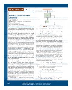
Consider the vibrating mechanical system shown in Fig. 1, which consists of an active undamped dynamic vibration absorber (secondary system) coupled to the perturbed mechanical system (primary system). The generalized coordinates are the displacements of both masses, x1 and x2 , respectively. In addition, u represents the force control input and f (t) some harmonic perturbation, possibly unknown. Here m1 , k1 and c1 denote mass, linear stiffness and linear viscous damping on the primary system, respectively. Similarly, m2 , k2 and c2 denote mass, stiffness and viscous damping of the dynamic vibration absorber. Note also that, when u ≡ 0 the active vibration absorber becomes only a passive vibration absorber.

f(t) = F0 sin wt

Mechanical System m1

k2

x1

c2 = 0

k1

c1 » 0

m2 u

x2

Active Vibration Absorber Fig. 1. Schematic diagram of the vibrating mechanical system with active vibration absorber. The mathematical model of this two degrees-of-freedom system is described by the following two coupled ordinary differential equations m1 x¨1 + c1 x˙ 1 + k1 x1 + k2 ( x1 − x2 ) = f (t) m2 x¨2 + k2 ( x2 − x1 ) = u (t)

(1)

where f (t) = F0 sin ωt, with F0 and ω denoting the amplitude and frequency of the excitation force, respecively. In order to simplify the analysis we have assumed that c1 ≈ 0.

30

Vibration Analysis and Control – New Trends and Development Vibration Control

4

Defining the state variables as z1 = x1 , z2 = x˙ 1 , z3 = x2 and z4 = x˙ 2 , one obtains the following state-space description z˙ 1 = z2 z˙ 2 = − k1m+1k2 z1 −

c1 m1 z2

+

k2 m1 z3

z˙ 3 = z4 z˙ 4 =

k2 m2 z1

+

1 m1

f (t) (2)

−

k2 m2 z3

+

1 m2 u ( t )

y = z1 It is easy to verify that the system (2) is completely controllable and observable as well as marginally stable in case of c1 = 0, f ≡ 0 and u ≡ 0 (asymptotically stable when c1 > 0). Note that, an immediate consequence is that, the output y = z1 has relative degree 4 with respect to u and relative degree 2 with respect to f and, therefore, the so-called disturbance decoupling problem of the perturbation f (t) from the output y = z1 , using state feedback, is not solvable (Isidori, 1995). To cancel the exogenous harmonic vibrations on the primary system, the dynamic vibration absorber should apply an equivalent force to the primary system, with the same amplitude but in opposite phase (sign). This means that the vibration energy injected to the primary system, by the exogenous vibration f (t), is transferred to the vibration absorber through the coupling elements (i.e., spring k2 ). Of course, this vibration control method is possible under the assumption of perfect knowledge of the exogenous vibrations and stable operating conditions (Preumont, 1993). In this work we will apply the algebraic identification method to estimate the parameters associated to the harmonic force f (t) and then, propose the design of an active vibration controller based on state feedback and feedforward information of f (t). 2.2 Passive vibration absorber

It is well known that a passive vibration absorber can only cancel the vibration f (t) affecting the primary system if and only if the excitation frequency ω coincides with the uncoupled natural frequency of the absorber (Den Hartog, 1934), that is,  k2 ω2 = =ω (3) m2 See Fig. 2, where X1 denotes the steady-state maximum amplitude of x1 (t) and δst the static deflection of the primary system under the constant force F0 . Note, however, that the interconnection of the passive vibration absorber to the primary system slightly changes the natural frequencies in both uncoupled subsystems and, hence, when ω = ω2 and close to those resonant frequencies the amplitudes might be large or theoretically infinite. This situation clearly leads to large displacements and could damage of any physical system. In what follows we shall use an active vibration absorber based on Generalized PI control (GPI) to provide some robustness with respect to variations on the excitation frequency ω, uncertain system parameters and initial conditions.

315

Design of Vibration ActiveAbsorbers Vibration Absorbers Using On-Line Design of Active Using On-line Estimation of Parameters and SignalsEstimation of Parameters and Signals

5 Without Vibration Absorber 4 With Passive Vibration Absorber

|X1/dst |

3

Vibration Cancellation at the Tuning Frequency of the Absorber w 2

2

1

0 0

0.2

0.4

0.6

0.8

1 w/w

1.2

1.4

1.6

1.8

2

2

Fig. 2. Frequency response of the vibrating mechanical system with passive vibration absorber. 2.3 Differential flatness

Because the system (2) is completely controllable from u then, it is differentially flat, with flat output given by y = z1 . Then, all the state variables and the control input can be differentially parameterized in terms of the flat output y and a finite number of its time derivatives (Fliess et al., 1993; Sira-Ramirez & Agrawal, 2004). In fact, from y and its time derivatives up to fourth order one can obtain that y = z1 y˙ = z2 y¨ = − k1m+1k2 z1 + y (3 )

=

y (4 ) =

− k1m+1k2 z2  (k 1 + k 2 )2 m21

k2 m1 z3 + mk21 z4 

+

k22 m1 m2

(4) z1 −



k 2 (k 2 +k 1 ) m21

+

k22 m1 m2



z3 +

k2 m1 m2 u

where c1 = 0 and f ≡ 0. Therefore, the differential parameterization results as follows z1 = y z2 = y˙ z3 = z4 =

k1 +k2 k2 y + k1 +k2 ˙+ k2 y 

m1 k 2 y¨ m 1 (3 ) k2 y

u = k 1 y + m1 + m2 +

(5) k1 k 2 m2



y¨ +

m 1 m 2 (4 ) k2 y

Then, the flat output y satisfies the following input-output differential equation y(4) = a0 y + a2 y¨ + bu

(6)

32

Vibration Analysis and Control – New Trends and Development Vibration Control

6

where k1 k2 m1 m2

k k1 + k2 a2 = − + 2 m1 m2 k2 b= m1 m2

a0 = −

From (6) one obtains the following differential flatness-based controller to asymptotically track some desired reference trajectory y∗ (t): u = b −1 (v − a0 y − a2 y¨ )

(7)

with

  v = (y∗ )(4) (t) − β6 y(3) − (y∗ )(3) (t) − β5 [y¨ − y¨∗ (t)] − β4 [y˙ − y˙ ∗ (t)] − β3 [y − y∗ (t)]

The use of this controller yields the following closed-loop dynamics for the trajectory tracking error e = y − y∗ (t): (8) e(4) + β6 e(3) + β5 e¨ + β4 e˙ + β3 e = 0 Therefore, selecting the design parameters β i , i = 3, ..., 6, such that the associated characteristic polynomial for (8) be Hurwitz, i.e., all its roots lying in the open left half complex plane, one can guarantee that the error dynamics be globally asymptotically stable. Nevertheless, this controller is not robust with respect to exogenous signals or parameter uncertainties in the model. In case of f (t) = 0, the parameterization should explicitly include the effect of f and its time derivatives up to second order. In addition, the implementation of this controller requires measurements of the time derivatives of the flat output up to third order and vibration signal and its time derivatives up to second order. Remark. In spite of the linear models under study, it results important to emphasize the great potential of the differential flatness approach for nonlinear flat systems, which can be analyzed using similar arguments (Fliess & Sira-Ramirez, 2003). In fact, the proposed results can be generalized to some classes of nonlinear mechanical systems. Next, we will synthesize two controllers based on the Generalized PI (GPI) control approach combined with differential flatness and passive absorption, in order to get robust controllers against external vibrations.

3. Generalized PI control 3.1 Control scheme using displacement measurement on the primary system

Since the system (2) is observable for the flat output y then, all the time derivatives of the flat output can be reconstructed by means of integrators, that is, they can be expressed in terms of the flat output y, the input u and iterated integrals of the input and the output variables (Fliess et al., 2002). t  For simplicity, we will denote the integral by ϕ and 0 ϕ ( τ ) dτ  t  σ1  (n)  σn−1 ϕ (σn ) dσn · · · dσ1 by ϕ with n a positive integer. The integral input-output 0 0 ··· 0

Design of Vibration ActiveAbsorbers Vibration Absorbers Using On-Line Design of Active Using On-line Estimation of Parameters and SignalsEstimation of Parameters and Signals

337

parameterization of the time derivatives of the flat output is given, modulo initial conditions, by  (3 )   (3) y + a2 y + b u y˙ = a0  (2 )  (2 ) (9) y + a2 y + b u y¨ = a0   (3 ) = a y˙ + b u y 0 y + a2 These expressions were obtained by successive integrations of the last equation in (6). For non-zero initial conditions, the relations linking the actual values of the time derivatives of the flat output to the structural estimates in (9) are given as follows y˙ + e12 t2 + e11 t + e11 y˙ = y¨ = y¨ + g11 t + g10

(10)

( 3) + h t2 + h t + h y(3) = y 12 11 10

where e1i , g j , hi , i = 0, . . . , 2, j = 0, . . . , 1, are real constants depending on the unknown initial conditions. For the design of the GPI controller, the time derivatives of the flat output are replaced for their structural estimates (9) into (7). This, however, implies that the closed-loop system would be actually excited by constant values, ramps and quadratic functions. To eliminate these destabilizing effects of such structural estimation errors, one can use the following controller with iterated integral error compensation:   u = b −1 v − a0 y − a2 y¨       ∗ (3 ) − ( y ∗ ) (3 ) ( t ) − β v = (y∗ )(4) (t) − β6 y y˙ − y˙ ∗ ( t) 5 y¨ − y¨ ( t ) − β4

− β3 [ y − y∗ (t)] − β2 ξ 1 − β1 ξ 2 − β0 ξ 3

(11)

ξ˙1 = y − y∗ ( t) , ξ 1 (0) = 0 ξ˙2 = ξ 1 ,

ξ 2 (0) = 0

ξ˙3 = ξ 2 ,

ξ 3 (0) = 0

The use of this controller yields the following closed-loop system dynamics for the tracking error, e = y − y∗ (t), described by e(7) + β6 e(6) + β5 e(5) + β4 e(4) + β3 e(3) + β2 e¨ + β1 e˙ + β0 e = 0

(12)

The coefficients β i , i = 0, ..., 6, have to be selected in such way that the characteristic polynomial of (12) be Hurwitz. Thus, one can conclude that lim e (t) = 0, i.e., the asymptotic output tracking of the reference trajectory lim y (t) = y∗ (t).

t→ ∞

t→ ∞

3.1.1 Robustness analysis with respect to external vibrations

Now, consider that the passive vibration absorber is tuned at the uncoupled natural frequency of the primary system, that is, ω2 = ω1 . The transfer function of the closed-loop system from

34

Vibration Analysis and Control – New Trends and Development Vibration Control

8

the perturbation f (t) to the output y = z1 is then given by x1 ( s ) f( s)   μ m2 s2 + k2 m2 s3 + β6 m2 s2 + β5 m2 s − β6 k2 μ − 2β6 k2 + β4 m2 − 2k2 s − k2 sμ (13)   = m32 s7 + β6 s6 + β5 s5 + β4 s4 + β3 s3 + β2 s2 + β1 s + β0

G (s) =

where μ = m2 /m1 is the mass ratio. Then, for the harmonic perturbation f (t) = F0 sin ωt, the steady-state magnitude of the primary system is computed as  μ A(ω ) (14) | X1 | = 3 F0 B (ω ) m2 where

 2   2 A ( ω ) = k 2 − m2 ω 2 − β6 m2 ω 2 − β6 k2 μ − 2β6 k2 + β4 m2 2   + − m2 ω 3 + β5 m2 ω − 2k2 ω − k2 ωμ 2  2  B (ω ) = − β6 ω 6 + β4 ω 4 − β2 ω 2 + β0 + − ω 7 + β5 ω 5 − β3 ω 3 + β1 ω

 k2 Note that X1 ≡ 0 exactly when ω = ω2 = m2 , independently of the selected gains of the control law in (11), corresponding to the dynamic performance of the passive vibration control scheme. This clearly corresponds to a finite zero in the above transfer function G (s), situation where the passive vibration absorber is well tuned. Thus, the control objective for (11) is to add some robustness when ω = ω2 and improve the performance of the closed-loop system using small control efforts and taking advantage of the passive vibration absorber (when ω = ω2 the system can operate with u ≡ 0). In Fig. 3 we can observe that, the active vibration absorber can attenuate vibrations for any excitation frequency, including vibrations with multiple harmonic signals. In fact, it is still possible to minimize the attenuation level by adding a proper viscous damping to the absorber (Korenev & Reznikov, 1993; Rao, 1995). 3.2 Control scheme using displacement measurement on the primary system and excitation frequency

Consider the perturbed system (2). The state variables and the control input u can be expressed in terms of the flat output y, the perturbation f and their time derivatives: z1 = y z2 = y˙ z3 =

k1 +k2 m1 1 ¨ k2 y + k2 y − k2

f (t)

k1 +k2 m 1 (3 ) k 2 y˙ + k 2 y

1 k2

− f˙ (t)  2 (4 ) m1 + m2 + u = mk1 m y + k y + 1 2

z4 =

(15)

k1 k 2 m2



y¨ − f (t) −

m2 k2

f¨ ( t)

Design of Vibration ActiveAbsorbers Vibration Absorbers Using On-Line Design of Active Using On-line Estimation of Parameters and SignalsEstimation of Parameters and Signals

359

6

5

|X1/dst |

4

3

2

Vibration Cancellation at the Tuning Frequency of the Absorber w 2

1

0 0

0.5

1

w/w

1.5

2

2.5

2

Fig. 3. Frequency response of the vibrating mechanical system using an active vibration absorber with controller (11). Furthermore, when f (t) = F0 sin ωt the flat output y satisfies the following input-output differential equation: y (4 ) = −

k1 k2 y− m1 m2



k k1 + k2 + 2 m1 m2



y¨ +

ω2 k2 − m1 m2 m1

F0 sin ωt +

k2 u m1 m2

(16)

Taking two additional time derivatives of (16) results in y (6 ) = −

k1 k2 y¨ − m1 m2



k k1 + k2 + 2 m1 m2



y (4 ) +

k2 u¨ − m1 m2



ω2 k2 − m1 m2 m1

Multiplication of (16) by ω 2 and adding it to (17) leads to   y(6) + d1 y(4) + d2 y¨ + d3 y = d4 u¨ + ω 2 u where

d1 = k1m+1k2 + mk22 +ω 2 d2 = k1m+1k2 + mk22 ω 2 + d3 = d4 =

ω 2 F0 sin ωt

(17)

(18)

k1 k2 m1 m2

k1 k2 2 m1 m2 ω k2 m1 m2

A differential flatness-based dynamic controller, using feedback measurements of the flat output y and its time derivatives up to fifth order as well as feedforward measurements of the excitation frequency ω, is proposed by the following dynamic compensator:   u¨ + ω 2 u = d4−1 v + d4−1 d1 y(4) + d2 y¨ + mk11 km22 ω 2 y       (19) v = y∗(6) − α10 y(5) − y∗(5) − α9 y(4) − y∗(4) − α8 y(3) − y∗(3)

− α7 [y¨ − y¨∗ ] − α6 [y˙ − y˙ ∗ ] − α5 [ y − y∗ ]

36

10

Vibration Analysis and Control – New Trends and Development Vibration Control

with zero initial conditions (i.e., u (0) = u˙ (0) = 0). It is important to remark that, the above differential equation resembles an exosystem (linear oscillator) tuned at the known excitation frequency ω (feedforward action) and injected by feedback terms involving the flat output y and its desired reference trajectory y∗ . On the other hand, one can note that the time derivatives of the flat output admit an integral input-output parameterization, obtained after some algebraic manipulations, given by

  (3 )  (5 )  (3 ) y˙ = − d1 y − d2 y − d3 y + d4 u  (2 )  (4 )  (2 )  (4 ) y¨ = − d1 y − d2 y − d3 y + d4 u + d4 ω 2 u     (3 ) (3 ) y + d4 u + d4 ω 2 u y˙ − d2 y − d3 y (3) = − d1  (2 )  (2 ) y (4) = − d1 y + d4 u + d4 ω 2 y¨ − d2 y − d3   u y (5) = − d1 y (3) − d2 y˙ − d3 y + d4 u˙ + d4 ω 2 u

(20)

The differences in the structural estimates of the time derivatives of the flat output with respect to the actual time derivatives are given by y˙ + p4 t4 + p3 t3 + p2 t2 + p1 t + p0 y˙ = y¨ = y¨ + p4 t3 + p3 t2 + p2 t + p1 y(3) = y (3) + q4 t4 + q3 t3 + q2 t2 + q1 t + q0 y(4) = y (4) + r3 t3 + r2 t2 + r1 t + r0 y(5) = y (5) + s4 t4 + s3 t3 + s2 t2 + s1 t + s0 where pi , q i , r j , si , i = 0,...,4, j = 0, ..., 3, are real constants depending on the unknown initial conditions. Finally, the differential flatness based GPI controller is obtained by replacing the actual time derivatives of the flat output in (19) by their structural estimates in (20) but using additional iterated integral error compensations as follows   u¨ + ω 2 u = d4−1 v + d4−1 d1 y (4) + d2 y¨ + d3 y      

(5) − y∗(5) − α y (4) − y∗(4) − α y (3) − y∗(3) v = y∗(6) − α10 y 9 8     − α7 y¨ − y¨∗ − α6 y˙ − y˙ ∗ − α5 [y − y∗ ] − α4 ξ 1 − α3 ξ 2 − α2 ξ 3 − α1 ξ 4 − α0 ξ 5 (21) ξ˙1 = y − y∗ , ξ 1 (0) = 0 ξ˙2 = ξ 1 , ξ 2 (0) = 0 ξ˙3 = ξ 2 , ξ 3 (0) = 0 ξ˙4 = ξ 3 , ξ 4 (0) = 0 ξ˙5 = ξ 4 , ξ 5 (0) = 0 This feedback and feedforward active vibration controller depends on the measurements of the flat output y and the excitation frequency ω, therefore, this dynamic controller can compensate simultaneously two harmonic components, corresponding to the tuned (passive) vibration absorber (ω2 ) and the actual excitation frequency (ω).

Design of Vibration ActiveAbsorbers Vibration Absorbers Using On-Line Design of Active Using On-line Estimation of Parameters and SignalsEstimation of Parameters and Signals

37 11

The closed-loop system dynamics, expressed in terms of the tracking error e = y − y∗ (t), is described by e(11) + α10 e(10) + α9 e(9) + α8 e(8) + α7 e(7) + α6 e(6) + α5 e(5) + α4 e(4) + α3 e(3) + α2 e¨ + α1 e˙ + α0 e = 0

(22)

Therefore, the design parameters αi , i = 0, ..., 10, have to be selected such that the associated characteristic polynomial for (22) be Hurwitz, thus guaranteeing the desired asymptotic output tracking when one can measure the excitation frequency ω. 3.2.1 Robustness with respect to external vibrations

Fig. 4 shows the frequency response of the closed-loop system, using an active vibration absorber based on differential flatness and measurements of y and ω. Note that this active 7 k1 = 1000 [N/m] m = 10 [Kg] 1 k2 = 200 [N/m] m2 = 2 [Kg]

6

1 st

|X /d |

5 4 3 2

Vibration Cancellation at the Tuning Frequency of the Absorber w

Vibration Cancellation at w s/w 1 = 0.8

2

1 0 0

0.5

1

w /w

1.5

2

2.5

2

Fig. 4. Frequency response of the vibrating mechanical system using the active vibration absorber with controller (21). vibration absorber employs the measurement of the excitation frequency ω and, therefore, such harmonic vibrations can always be cancelled (i.e., X1 = 0). Moreover, this absorber is also useful to eliminate vibrations of the form f (t) = F0 [sin (ω s t) + sin (ω2 t)], where ω s is the measured frequency (affecting the feedforward control action) and ω2 is the design frequency of the passive absorber. 3.3 Simulation results

Some numerical simulations were performed on a vibrating mechanical platform from Educational Control Products (ECP), model 210/210a Rectilinear Control System, characterized by the set of system parameters given in Table 1. The controllers (11) and (21) were specified in such a way that one could prove how the active vibration absorber cancels the two harmonic vibrations affecting the primary system and the asymptotic output tracking of the desired reference trajectory.

38

Vibration Analysis and Control – New Trends and Development Vibration Control

12

m1 = 10kg m2 = 2kg N k1 = 1000 N m k 2 = 200 m N N c1 ≈ 0 m/s c2 ≈ 0 m/s Table 1. System parameters for the primary and secondary systems. The planned trajectory for the flat output y = z1 is given by ⎧ 0 for 0 ≤ t < T1 ⎨ ∗ y (t) = ψ (t, T1 , T2 ) y¯ for T1 ≤ t ≤ T2 ⎩ y¯ for t > T2 where y¯ = 0.01m, T1 = 5s, T2 = 10s and ψ ( t, T1 , T2 ) is a Bézier polynomial, with ψ ( T1 , T1 , T2 ) = 0 and ψ ( T2 , T1 , T2 ) = 1, described by

5 



2

5  t − T1 t − T1 t − T1 t − T1 ψ (t) = + r3 − ... − r6 r1 − r2 T2 − T 1 T2 − T 1 T2 − T 1 T2 − T 1 with r1 = 252, r2 = 1050, r3 = 1800, r4 = 1575, r5 = 700, r6 = 126. Fig. 5 shows the dynamic behavior of the closed-loop system with the controller (11). One can observe the vibration cancellation on the primary system and the output tracking of the pre-specified reference trajectory. The controller gains were chosen so that the characteristic polynomial of the closed-loop tracking error dynamics (12) is a Hurwitz polynomial given by  3 2 pd1 (s) = (s + p1 ) s2 + 2ζ 1 ω n1 s + ω n1

0.015

0.08

0.01

0.06 0.04

0.005

z3 [m]

z1 [m]

with ζ 1 = 0.5, ω n1 = 12rad/s, p1 = 6.

0

0

-0.005 -0.01 0

0.02

-0.02 2

4

6 time [s]

8

10

12

2

4

6 time [s]

8

10

12

-0.04 0

2

4

6 time [s]

8

10

15

u [N]

10 5 0 -5 0

Fig. 5. Active vibration absorber using measurements of y and ω for harmonic vibration f = 2 sin (10t) N.

12

39 13

Design of Vibration ActiveAbsorbers Vibration Absorbers Using On-Line Design of Active Using On-line Estimation of Parameters and SignalsEstimation of Parameters and Signals

Fig. 6 shows the robust performance of closed-loop system employing the controller (21). One can see that the active vibration absorber eliminates vibrations containing two different harmonics. The design parameters were selected to have a sixth order closed-loop characteristic polynomial  5 2 pd2 (s) = (s + p2 ) s2 + 2ζ 2 ω n2 s + ω n2 with

ζ 2 = 0.5,

ω n2 = 10rad/s,

p2 = 5.

0.015

0.1

0.01

0.05 z3 [m]

z1 [m]

0.005 0

0

-0.005 -0.05 -0.01 -0.015 0

2

4

6 time [s]

8

10

12

2

4

6 time [s]

8

10

12

-0.1 0

2

4

6 time [s]

8

10

12

15

u [N]

10 5 0 -5 -10 0

Fig. 6. Active vibration absorber using measurements of y and ω, for external vibration f = 2 [sin (8.0109t) + sin (10t)] N.

4. Algebraic identification of harmonic vibrations The algebraic identification methodology (Fliess & Sira-Ramirez, 2003) can be applied to estimate the parameters associated to exogenous harmonic vibrations affecting a mechanical vibrating system (Beltran et al., 2004). To do that, consider the input-output differential equation (16), where only displacement measurements of the primary system y = z1 and the control input u are available for the identification process of the parameters associated with the harmonic signal f (t) = F0 sin ωt, that is,



k k k ω2 k2 k1 + k2 k2 F0 sin ωt + y (4 ) = − 1 2 y − + 2 y¨ + − u (23) m1 m2 m1 m2 m1 m2 m1 m1 m2 Next we will proceed to synthesize two algebraic identifiers for the excitation frequency ω and amplitude F0 .

40

Vibration Analysis and Control – New Trends and Development Vibration Control

14

4.1 Identification of the excitation frequency ω

The differential equation (23) is expressed in notation of operational calculus as

m k k k m1 s4 Y ( s ) + k 1 + k 2 + 1 2 s2 Y ( s ) + 1 2 Y ( s ) m2 m2

k ω k2 − ω 2 F0 2 + a3 s3 + a2 s2 + a1 s + a0 = 2 U (s) + m2 m2 s + ω2

(24)

where ai , i = 0,...,3, denote unknown real constants  depending on the system initial conditions. Now, equation (24) is multiplied by s2 + ω 2 , leading to



    k k s2 + ω 2 s4 Y + 2 s2 Y m1 + s2 Y + 2 Y k 1 + k 2 s2 Y m2 m2

     k k2 (25) = 2 s2 + ω 2 u + − ω 2 F0 ω + s2 + ω 2 a3 s3 + a2 s2 + a1 s + a0 m2 m2 This equation is then differentiated six times with respect to s, in order to eliminate the constants ai and the unknown amplitude F0 . The resulting equation is then multiplied by s−6 to avoid differentiations with respect to time in time domain, and next transformed into the time domain, to get     a11 (t) + ω 2 a12 (t) m1 + a12 (t) + ω 2 b12 (t) k1 = c1 (t) + ω 2 d1 (t) (26) where Δt = t − t0 and a11 (t) = m2 g11 (t) + k2 g12 (t) a12 (t) = m2 g12 (t) + k2 g13 (t) b12 (t) = m2 g13 (t) + k2

 (6 ) t0

(Δt)6 z1

c1 (t) = k2 g14 (t) − k2 m2 g12 (t) d1 ( t ) = k 2

 (6) t0

(Δt)6 u − k2 m2 g13 (t)

with g11 (t) = 720

 (6 ) t0

+450 g12 (t) = 360

 (2 ) t0

 (6 )

−24

y−4320

t0

(Δt) y+5400

t0

(Δt)4 y−36

(Δt)2 y−480

 (3 ) t0

 (5 )

(Δt)5 y+

 t0

 (2 ) t0

t0

(Δt)2 y−2400

( Δt)5 y+ (Δt)6 y

 (5 ) t0

 (4 )

(Δt)3 y+180

( Δt)6 y

 (4 ) t0

(Δt)4 y

 (3 ) t0

(Δt)3 y

Design of Vibration ActiveAbsorbers Vibration Absorbers Using On-Line Design of Active Using On-line Estimation of Parameters and SignalsEstimation of Parameters and Signals

g13 (t) = 30 g14 (t) = 30

 (6 ) t0

 (6 ) t0

 (5 )

(Δt)4 y−12

(Δt)5 y+

t0

(Δt)4 u −12

 (5 )

(Δt)5 u +

t0

 (4 ) t0

 (4 ) t0

41 15

(Δt)6 y (Δt)6 u

Finally, solving for the excitation frequency ω in (26) leads to the following on-line algebraic identifier: N (t) c (t) − a11 (t) m1 − a12 (t) k1 ω e2 = 1 (27) = 1 D1 (t) a12 (t) m1 + b12 (t) k1 − d1 (t) This estimation is valid if and only if the condition D1 (t) = 0 holds in a sufficiently small time interval (t0 , t0 + δ0 ] with δ0 > 0. This nonsingularity condition is somewhat similar to the well-known persistent excitation property needed by most of the asymptotic identification methods (Isermann & Munchhof, 2011; Ljung, 1987; Soderstrom, 1989). In particular, this obstacle can be overcome by using numerical resetting algorithms or further integrations on N1 (t) and D1 (t) (Sira-Ramirez et al., 2008). 4.2 Identification of the amplitude F0

To synthesize an algebraic identifier for the amplitude F0 of the harmonic vibrations acting on the mechanical system, the input-output differential equation (23) is expressed in notation of operational calculus as follows

m k k k m1 s4 Y ( s ) + k 1 + k 2 + 1 2 s2 Y ( s ) + 1 2 Y ( s ) m2 m2

k2 k2 U (s) + − ω 2 F ( s ) + a3 s3 + a2 s2 + a1 s + a0 (28) = m2 m2 Taking derivatives, four times, with respect to s makes possible to remove the dependence on the unknown constants ai . The resulting equation is then multiplied by s−4 , and next transformed into the time domain, to get

 (4 ) m k k k m1 P1 (t) + k1 + k2 + 1 2 P2 (t) + 1 2 (Δt)4 z1 m2 m 2 t0

 (4 )  (4 ) k k2 = 2 − ω2 (Δt)4 u + F0 (Δt)4 sin ωt m 2 t0 m2 t0

(29)

where P1 (t) = 24 P2 (t) = 12

 (4 ) t0

 (4 ) t0

z1 − 96

 (3 ) t0

(Δt)2 z1 − 8

(Δt) z1 + 72  (3) t0

 (2 ) t0

(Δt)3 z1 +

(Δt)2 z1 − 16

 (2 ) t0

 t0

(Δt)3 z1 + (Δt)4 z1

(Δt)4 z1

It is important to note that equation (29) still depends on the excitation frequency ω, which can be estimated from (27). Therefore, it is required to synchronize both algebraic identifiers for ω and F0 . This procedure is sequentially executed, first by running the identifier for ω and, after some small time interval with the estimation ω e (t0 + δ0 ) is then started the algebraic identifier

42

Vibration Analysis and Control – New Trends and Development Vibration Control

16

for F0 , which is obtained by solving N2 (t) − D2 (t) F0 = 0

(30)

where

 (4 )  (4 ) m1 k 2 k k k P2 (t) + 1 2 N2 (t) = m1 P1 (t) + k1 + k2 + (Δt)4 z1 − 2 (Δt)4 u m2 m2 t0 +δ0 m2 t0 +δ0

 (4 ) k2 D2 (t) = − ω e2 (Δt)4 sin [ω e (t0 + δ0 )t] m2 t0 + δ0 In this case if the condition D2 (t) = 0 is satisfied for all t ∈ (t0 + δ0 , t0 + δ1 ] with δ1 > δ0 > 0, then the solution of (30) yields an algebraic identifier for the excitation amplitude F0e =

N2 (t) , ∀t ∈ (t0 + δ0 , t0 + δ1 ] D2 (t)

(31)

4.3 Adaptive-like active vibration absorber for unknown harmonic forces

The active vibration control scheme (21), based on the differential flatness property and the GPI controller, can be combined with the on-line algebraic identification of harmonic vibrations (27) and (31), where the estimated harmonic force is computed as f e (t) = F0e sin(ω e t)

(32)

resulting some certainty equivalence feedback/feedforward control law. Note that, according to the algebraic identification approach, providing fast identification for the parameters associated to the harmonic vibration (F0 , ω) and, as a consequence, a fast estimation of this perturbation signal, the proposed controller is similar to an adaptive control scheme. From a theoretical point of view, the algebraic identification is instantaneous (Fliess & Sira-Ramirez, 2003). In practice, however, there are modelling errors and many other factors that complicate the real-time algebraic computation. Fortunately, the identification algorithms and closed-loop system are robust against such difficulties. 4.4 Simulation results

Fig. 7 shows the identification process of the excitation frequency of the resonant harmonic perturbation f (t) = 2 sin (8.0109t) N and the robust performance of the adaptive-like control scheme (21) for reference trajectory tracking tasks, which starts using the nominal frequency value ω = 10rad/s, which corresponds to the known design frequency for the passive vibration absorber, and at t > 0.1s this controller uses the estimated value of the resonant excitation frequency. Here it is clear how the frequency identification is quickly performed (before t = 0.1s and it is almost exact with respect to the actual value. One can also observe that, the resonant vibrations affecting the primary mechanical system are asymptotically cancelled from the primary system response in a short time interval. It is also evident the presence of some singularities in the algebraic identifier, i.e., when its denominator D1 (t) is zero. The first singularity, however, occurs about t = 0.727s, which is too much time (more than 7 times) after the identification has been finished.

43 17

Design of Vibration ActiveAbsorbers Vibration Absorbers Using On-Line Design of Active Using On-line Estimation of Parameters and SignalsEstimation of Parameters and Signals

Fig. 8 illustrates the fast and effective performance of the on-line algebraic identifier for the amplitude of the harmonic force f (t) = 2 sin (8.0109t) N. First of all, it is started the identifier for ω, which takes about t < 0.1s to get a good estimation. After the time interval (0, 0.1]s, where t0 = 0s and δ0 = 0.1s with an estimated value ω e (t0 + δ0 ) = 8.0108rad/s, it is activated the identifier for the amplitude F0 . -7

-5

10

3 2

4 2

N1

0.1 time [s]

0.15

0

-1

-2 -4 0.25

0.5

-6 0

0.75

15

0.1

10

-0.01

u [N]

0.15

0

0.05 0

10

15

0.5

0.75

10

15

time [s]

0.01

5

0.25

time [s]

0.02

-0.02 0

D1

2

0

-3 0

0.2

x 10

4

-2 0.05

z3 [m]

z1 [m]

6

1

6

e

w [rad/s]

8

0 0

x 10

5 0

-0.05 0

5

time [s]

10

15

-5 0

5

time [s]

time [s]

Fig. 7. Controlled system responses and identification of frequency for f (t) = 2 sin (8.0109t) [N]. -5

2.5

2.5

-6

x 10

12

x 10 D2

N2 2

2

8 1.5

F0e

1.5 1

4

1 0.5 0 0.5

0 0

0

0.05

0.1 t [s]

0.15

0.2

-0.5 0

0.25

0.5

0.75

t [s]

-4 0

0.25

0.5

0.75

t [s]

Fig. 8. Identification of amplitude for f (t) = 2 sin (8.0109t) [N]. One can also observe that the first singularity occurs when the numerator N2 (t) and denominator D2 (t) are zero. However the first singularity is presented about t = 0.702s, and therefore the identification process is not affected.

44

Vibration Analysis and Control – New Trends and Development Vibration Control

18

Now, Figs. 9 and 10 present the robust performance of the on-line algebraic identifiers for the excitation frequency ω and amplitude F0 . In this case, the primary system was forced by external vibrations containing two harmonics, f (t) = 2 [sin (8.0109t) + 10 sin (10t)] N. Here, the frequency ω2 = 10rad/s corresponds to the known tuning frequency of the passive vibration absorber, which does not need to be identified. Once again, one can see the fast and effective estimation of the resonant excitation frequency ω = 8.0109rad/s and amplitude F0 = 2N as well as the robust performance of the proposed active vibration control scheme (21) based on differential flatness and GPI control, which only requires displacement measurements of the primary system and information of the estimated excitation frequency. -5

10

2.5

6

1 4

0.5

0 0

0 0.05

0.1 t [s]

0.15

-0.5 0

0.2

0.25

0.5

0.75

0.1

0.01

0.05 z3 [m]

0.02

0 -0.01

5

10

15

0.5

0.75

10

15

t [s] 15 10

0 -0.05

-0.02 0

0.25

t [s]

u [N]

e

w [rad/s]

1.5

2

z1 [m]

x 10 3.5 3 D1 2.5 2 1.5 1 0.5 0 -0.5 0

N1

2

8

-7

x 10

5 0 -5

-0.1 0

5

t [s]

10

15

-10 0

5

t [s]

t [s]

Fig. 9. Controlled system responses and identification of the unknown resonant frequency for . f (t) = 2 [sin (8.0109t) + 10 sin (10t)] [N]. -5

2.5

2.5

-6

x 10

12

N2

D2 10

2

2

x 10

8 1.5 1.5 F0e

6 1 4

1 0.5

2 0.5

0 0

0

0.05

0.1 t [s]

0.15

0.2

-0.5 0

0

0.25

0.5 t [s]

0.75

-2 0

0.25

0.5 t [s]

Fig. 10. Identification of amplitude for f (t) = 2 [sin (8.0109t) + 10 sin (10t)] [N].

0.75

Design of Vibration ActiveAbsorbers Vibration Absorbers Using On-Line Design of Active Using On-line Estimation of Parameters and SignalsEstimation of Parameters and Signals

45 19

5. Conclusions In this chapter we have described the design approach of a robust active vibration absorption scheme for vibrating mechanical systems based on passive vibration absorbers, differential flatness, GPI control and on-line algebraic identification of harmonic forces. The proposed adaptive-like active controller is useful to completely cancel any harmonic force, with unknown amplitude and excitation frequency, and to improve the robustness of passive/active vibrations absorbers employing only displacement measurements of the primary system and small control efforts. In addition, the controller is also able to asymptotically track some desired reference trajectory for the primary system. In general, one can conclude that the adaptive-like vibration control scheme results quite fast and robust in presence of parameter uncertainty and variations on the amplitude and excitation frequency of harmonic perturbations. The methodology can be applied to rotor-bearing systems and some classes of nonlinear mechanical systems.

6. References Beltran-Carbajal, F., Silva-Navarro, G. & Sira-Ramirez, H. (2003). Active Vibration Absorbers Using Generalized PI and Sliding-Mode Control Techniques, Proceedings of the American Control Conference 2003, pp. 791-796, Denver, CO, USA. Beltran-Carbajal, F., Silva-Navarro, G. & Sira-Ramirez, H. (2004). Application of On-line Algebraic Identification in Active Vibration Control, Proceedings of the International Conference on Noise & Vibration Engineering 2004, pp. 157-172, Leuven, Belgium, 2004. Beltran-Carbajal, F., Silva-Navarro, G., Sira-Ramirez, H., Blanco-Ortega, A. (2010). Active Vibration Control Using On-line Algebraic Identification and Sliding Modes, Computación y Sistemas, Vol. 13, No. 3, pp. 313-330. Braun, S.G., Ewins, D.J. & Rao, S.S. (2001). Encyclopedia of Vibration, Vols. 1-3, Academic Press, San Diego, CA. Caetano, E., Cunha, A., Moutinho, C. & Magalhães, F. (2010). Studies for controlling human-induced vibration of the Pedro e Inês footbridge, Portugal. Part 2: Implementation of tuned mass dampers, Engineering Structures, Vol. 32, pp. 1082-1091. Den Hartog, J.P. (1934). Mechanical Vibrations, McGraw-Hill, NY. Fliess, M., Lévine, J., Martin, P. & Rouchon, P. (1993). Flatness and defect of nonlinear systems: Introductory theory and examples, International Journal of Control, Vol. 61(6), pp. 1327-1361. Fliess, M., Marquez, R., Delaleau, E. & Sira-Ramirez, H. (2002). Correcteurs Proportionnels-Integraux Généralisés, ESAIM Control, Optimisation and Calculus of Variations, Vol. 7, No. 2, pp. 23-41. Fliess, M. & Sira-Ramirez, H. (2003). An algebraic framework for linear identification, ESAIM: Control, Optimization and Calculus of Variations, Vol. 9, pp. 151-168. Fuller, C.R., Elliot, S.J. & Nelson, P.A. (1997). Active Control of Vibration, Academic Press, San Diego, CA. Isermann, R. & Munchhpf, M. (2011). Identification of Dynamic Systems, Springer-Verlag, Berlin. Isidori, A. (1995). Nonlinear Control Systems, Springer-Verlag, NY. Ljung, L. (1987). Systems Identification: Theory for the User, Prentice-Hall, Englewood Cliffs, NJ.

46

20

Vibration Analysis and Control – New Trends and Development Vibration Control

Korenev, B.G. & Reznikov, L.M. (1993). Dynamic Vibration Absorbers: Theory and Technical Applications, Wiley, London. Preumont, A. (2002). Vibration Control of Active Structures: An Introduction, Kluwer, Dordrecht, 2002. Rao, S.S. (1995). Mechanical Vibrations, Addison-Wesley, NY. Sira-Ramirez, H. & Agrawal, S.K. (2004). Differentially Flat Systems, Marcel Dekker, NY. Sira-Ramirez, H., Beltran-Carbajal, F. & Blanco-Ortega, A. (2008). A Generalized Proportional Integral Output Feedback Controller for the Robust Perturbation Rejection in a Mechanical System, e-STA, Vol. 5, No. 4, pp. 24-32. Soderstrom, T. & Stoica, P. (1989). System Identification, Prentice-Hall, NY. Sun, J.Q., Jolly, M.R., & Norris, M.A. (1995). Passive, adaptive and active tuned vibration ˝ a survey. In: Transaction of the ASME, 50th anniversary of the design absorbers U ˝ engineering division, Vol. 117, pp. 234U42. Taniguchi, T., Der Kiureghian, A. & Melkumyan, M. (2008). Effect of tuned mass damper on displacement demand of base-isolated structures, Engineering Structures, Vol. 30, pp. 3478-3488. Weber, B. & Feltrin, G. (2010). Assessment of long-term behavior of tuned mass dampers by system identification. Engineering Structures, Vol. 32, pp. 3670-3682. Wright, R.I. & Jidner, M.R.F. (2004). Vibration Absorbers: A Review of Applications in Interior Noise Control of Propeller Aircraft, Journal of Vibration and Control, Vol. 10, pp. 12211237. Yang, Y., Muñoa, J., & Altintas, Y. (2010). Optimization of multiple tuned mass dampers to suppress machine tool chatter, International Journal of Machine Tools & Manufacture, Vol. 50, pp. 834-842.