2476
IEEE TRANSACTIONS ON AUTOMATIC CONTROL, VOL. 55, NO. 11, NOVEMBER 2010
Design of Affine Controllers via Convex Optimization Joëlle Skaf, Member, IEEE, and Stephen P. Boyd, Fellow, IEEE
Abstract—We consider a discrete-time time-varying linear dynamical system, perturbed by process noise, with linear noise corrupted measurements, over a finite horizon. We address the problem of designing a general affine causal controller, in which the control input is an affine function of all previous measurements, in order to minimize a convex objective, in either a stochastic or worst-case setting. This controller design problem is not convex in its natural form, but can be transformed to an equivalent convex optimization problem by a nonlinear change of variables, which allows us to efficiently solve the problem. Our method is related to the classical -design procedure for time-invariant, infinite-horizon linear controller design, and the more recent purified output control method. We illustrate the method with applications to supply chain optimization and dynamic portfolio optimization, and show the method can be combined with model predictive control techniques when perfect state information is available. Index Terms—Affine controller, dynamical system, dynamic linear programming (DLP), linear exponential quadratic Gaussian (LEQG), linear quadratic Gaussian (LQG), model predictive control (MPC), proportional-integral-derivative (PID).
I. INTRODUCTION
W
E consider a discrete-time time-varying linear dynamical system operating over a finite horizon, perturbed by process noise, with linear noise corrupted measurements of the state, and a cost function that is convex in the state and input trajectories. We will consider two models of the process and measurement noises: stochastic, with the objective measured as the mean cost; and worst-case, in which the disturbances lie in a given set, and the objective is the maximum cost, over all possible disturbances. We require that the input or action must be causal, i.e., a function (or policy) of the previously observed measurements. With a stochastic noise model, the problem of finding a policy that minimizes the objective is the general stochastic control problem, also called stochastic optimization with recourse [3], [14], [18], [57], [75]. With a worst-case noise model, it is called robust optimization with recourse or robust dynamic programming [9], [11], [12], [78]. Even with linear dynamics and convex underlying cost function, the stochastic control problem is very difficult to solve. In the special case when noise-free measurements of the state are
Manuscript received April 30, 2008; revised September 26, 2008; accepted March 11, 2010. First published March 22, 2010; current version published November 03, 2010. This was work supported by the NSF award ECS-0423905, by NSF award 0529426, by DARPA award N66001-06-C-2021, by NASA award NNX07AEIIA, by AFOSR award FA9550-06-1-0514, and by AFOSR award FA9550-06-1-0312. Recommended by Associate Editor P. A. Parrilo. The authors are with the Information Systems Lab, Electrical Engineering Department, Stanford University, Stanford, CA 94305-9510 USA (e-mail:
[email protected];
[email protected];
[email protected]). Color versions of one or more of the figures in this paper are available online at http://ieeexplore.ieee.org. Digital Object Identifier 10.1109/TAC.2010.2046053
available, the optimal control policy is a function of the current state, which can, in principle, be determined by solving the dynamic programming or Bellman equation to find the cost-to-go function [4], [5]. While this gives us much insight, it does not lead to a practical method, except when the state dimension is very small (say, no more than 3). Another special case in which we obtain a practical solution is when the cost is quadratic and the disturbances are Gaussian, i.e., the linear quadratic Gaussian (LQG) problem. In this special case, the optimal control policy is affine, i.e., a linear function of the past measurements, plus a constant [2], [63]. Another case in which the optimal control policy is known, and affine, is when the cost is the exponential of a quadratic function, and the disturbances are Gaussian, which is the linear exponential quadratic Gaussian (LEQG) or risk-sensitive LQG problem [75, vol. 1, §19]. Many methods have been proposed to find suboptimal policies that can work well in practice. Perhaps the simplest methods are those from classical linear feedback control techniques, such as proportional-integral-derivative (PID) control [35]. One very effective technique that can be used when a noiseless measurement of the state is available is model predictive control (MPC) [6], [50], [53], [75], which goes by many other names, including dynamic matrix control [29], rolling horizon planning [28], and dynamic linear programming (DLP) [66]. MPC is based on solving a convex optimization problem at each step, with the unknown future disturbances replaced with estimates available at the current time (such as conditional means); but only the current action or input is used. At the next step, the same problem is solved, this time using the exact value of the current state, which is now known from the measurement. Another approach goes under the name approximate dynamic programming [13], [14], [55], in which some estimate of the optimal value function, or optimal policy, is found. While many of the methods assume that perfect state measurements are available, they can be used with an estimate of the state, obtained by an observer or state estimator [19]. (The optimal controller in the very special case of LQG can be expressed as an optimal state feedback, applied to an optimal estimate of the state; but in essentially all other cases, such a separation principle does not hold.) Of course, there are many custom methods for specific problems. In this paper we describe another method that yields a suboptimal controller, that, like many of the others listed above, can work well in practice. We limit our search to affine controllers, in which the control policy functions are all affine. Such controllers are characterized by a constant portion, and a set of controller gains that relate current and past measurements to the current input or action; in particular, they are parametrized by a finite number of real parameters. While affine policies are known to be optimal in the LQG case, they are certainly not optimal in the general case. In the language of stochastic programming with recourse, affine controllers are very specialized
0018-9286/$26.00 © 2010 IEEE
SKAF AND BOYD: DESIGN OF AFFINE CONTROLLERS VIA CONVEX OPTIMIZATION
and limited; the only recourse we have is linear in the measurements. While there is limited theoretical basis to expect that such controllers will work well (e.g., see [15] for proof of optimality of affine controllers in the context of one-dimensional, constrained, multi-stage robust optimization), examples suggest that in many cases they work quite well. This should not be too surprising, since PID control (a very special case of affine controllers) is widely used in industrial control. In any case, the point of this paper is not to endorse or recommend affine controllers, especially over the other suboptimal techniques described above. The main point of this paper is to show that the globally optimal affine controller can be effectively computed by convex optimization. More accurately, we reduce the problem to solving a convex stochastic or worst-case robust optimization problem. In some cases such problems can be solved exactly; in many others, an approximation method, such as sampling, must be used. These approximations can be made arbitrarily tight (at the cost of computational effort), and often yield very good results with nominal effort. Computing the optimal affine controller (coefficients) requires solving a single convex stochastic or worst-case robust optimization problem offline, so the time required to solve the problem is not critical. When the affine controller is running online, the computational load is extremely small, and consists of evaluating an affine function of the observed outputs; thus, the affine controller can be run online at very high speeds, if needed. In contrast, MPC methods require solving an optimization problem at each time step, i.e., online. The affine controller design problem is not convex in its natural form, but can be transformed to an equivalent convex optimization problem by a nonlinear change of variables, which allows us to efficiently solve the problem. Our method is related to the classical -design procedure, or Youla parametrization [76], [77] for time-invariant, infinite-horizon linear controller design [1], [32], [33], [45], [47], [49], [73]. The book [20] and survey paper [21] describes this method, and the use of convex optimization to design continuous-time, time-invariant controllers, in detail; the Notes and References trace the ideas back into the 1960s. The books [30], [34] use these methods to minimize the worst-case output, with unknown but bounded input, which can be cast (after -parametrization) as an norm minimization problem, and then solved using linear programming. The method is also related to the more recent purified output control method [7], [8]. While the method described in this paper is certainly related to the results given in these books and papers, the specifics are somewhat different. The design of affine controllers in the context of discrete-time systems has received recent attention. It has been addressed in the context of robust optimization and robust controller design in [7], [8], [10], in the context of receding horizon control in [58], [59], for single-asset multistage investments with affine recourse and transaction costs in [67], for portfolio allocation problems with affine recourse in [24], for improved linear decision rules for stochastic programming in [27], and in the context of decentralized control over Banach spaces in [60]. We now mention what we believe is the closest work to the methods described in this paper, in the stochastic noise model setting. In the unpublished report [46], Hansson et al. describe a -parametrization method for computing an affine controller, for a static (i.e., nondynamic) problem that satisfies some
2477
second moment stochastic constraints, which can be expressed exactly (in the transformed variables) using second-order cone constraints. In a series of papers [68]–[71], van Hessen and Bosgra describe -parametrization methods for stochastic affine recourse MPC methods (as in our Section VIII). They approximate stochastic constraints, including chance constraints, as second moment constraints, which then translate into second-order cone constraints. Sung [64] applies their affine recourse MPC method to constrained portfolio optimization. Work similar in flavor to van Hessen’s and Bosgra’s was published by Wang et al. [74] and Goulart and Kerrigan [42] in which -parametrization is used to design affine recourse MPC methods for the special case of a convex quadratic objective function. We also mention the closest work to the methods described in this paper, in the worst-case noise model setting. The idea that a -parametrization-like method can be used for minimax controller design in MPC was introduced in [51], [52]. It was then analyzed and extended in [41], [43], where Goulart et al. describe and analyze a -parametrization method for computing affine state feedback control policies in the context of linear discrete-time systems, which are subject to unknown but bounded state disturbances and mixed constraints on the state and input. They also show that such a formulation results in a stabilizing control law. As described in the previous paragraphs, many of the ideas and techniques described in this paper are known, in general or other settings, such as infinite horizon, continuous-time timeinvariant systems. Our contribution is to work out these ideas in detail, in a particular setting: discrete-time, finite horizon, timevarying system, with general convex objective and constraint functions, and arbitrary disturbance distribution. As far as we know, the case presented here has not appeared in the literature. Although not directly related to our topic, we also mention two areas of research that share some similarities with our approach. Our method uses a (matrix) bilinear change of variables to convexify a non-convex controller design problem; this idea also came up in [39], [40], where a different change of variables is used to solve problems in the synthesis of state feedback gains, with LMI-based performance metric; see [22, §7.2.1]. The other area we mention is control-Lyapunov functions [36], [37], [56], [61], [62] in which a suboptimal control law can be found by convex optimization (in this case, over a set of approximate value functions). Finally, we mention that there is a large literature on multistage stochastic linear programming, which can be used to solve (exactly or approximately) some versions of our problem (with piecewise linear objectives and polyhedral constraints); see [16], [17], [26], [31], [38], [44], [48], [65], [72]. The proposed methods range from decomposition and partitioning methods to sampling-based approximation algorithms, and are usually limited to short horizons. In Sections II and III, we describe our model and the controller design problem in detail. We derive the formulas that relate the disturbances to the state and inputs in Section IV, and in Section V, we describe our convex formulation of the controller design problem. In the next two sections we illustrate the method with applications: a supply chain optimization problem in Section VI, and a dynamic portfolio optimization problem in Section VII. In Section VIII, we explain how the affine con-
2478
IEEE TRANSACTIONS ON AUTOMATIC CONTROL, VOL. 55, NO. 11, NOVEMBER 2010
troller synthesis method can be combined with a model predictive control technique. II. SYSTEM MODEL We consider a discrete-time linear time-varying system (or , with dynamics plant), over the time interval (1) is the system state, is the process where noise or exogenous input, and is the control input, all at time step . The sensor or measured output is given by (2) where , and is the sensor noise at time period . We will also be interested in the special case of perfect state measurements, in which and , i.e., , for . With slight abuse of notation, we will use , , , , and to denote the associated trajectories
We define
, with
, and
where forms a block diagonal matrix from its arguments. The system (1) and (2) can then be written as
block strictly lower triangular. vanish, we say the matrix is (For , these correspond to the usual lower triangular and strictly lower triangular matrices.) We note for future use block strictly lower triangular, and is that is block strictly lower triangular. III. CONTROLLER DESIGN A. Causal and Affine Controllers We will consider causal output feedback controllers, for has the form which
The family of functions , for , is called the control policy. We will focus on the special case of affine causal output feedback, in are affine, i.e., have the form which the functions (4) (5) We refer to as the constant or open-loop part of the as the feedback control, and we refer to control gain. We interpret as the input we apply if all preas the vious measurements were zero, and we interpret control or recourse gain from measurement to input . If is small, for example, it means that our choice of is not heavily influenced by the measurement . We can also express the control law in ’shifted form’. Let be some (arbitrary) nominal value of the output signal. We can express the control law (4) as
(3) where
for
.. . .. .
..
.. . .. .
, where
In this form we interpret as the discrepancy between the measurement at time and the nominal output value at time . We interpret as the input we apply at time if all previous discrepancies were zero, i.e., all previous measurements were equal to their nominal values. We interpret as the gain from past discrepancies to the current input. In the perfect state measurement case, the controller reduces to an affine causal state feedback controller, for which is
.
..
.
(Entries not shown in these matrices are zero.) We say that a matrix is block lower triangular if it can be written as a block matrix with each block , and all blocks above the diagonal vanish. If in addition the diagonal blocks
Refer to as state feedback control gain. Once we fix the control policy, the input trajectory and the state trajectory are functions of and , the process and measurement noises. We will consider two generic types of problems, which differ in how the unknown process and noise disturbances are modeled.
SKAF AND BOYD: DESIGN OF AFFINE CONTROLLERS VIA CONVEX OPTIMIZATION
2479
IV. CLOSED-LOOP SYSTEM
B. Stochastic Control In the stochastic model, the process and sensor noises are random variables, with some known joint distribution. As a result, the input and state trajectories are also random variables. be a convex objective function Let of the state and input trajectories. We judge our control performance by the expected value of this objective function
We now derive the explicit dependence of and on and , when the controller is affine. We define feedback matrix as
.. . which is
where the expectation is over and . We treat constraints in a , similar way. Let be a set of convex constraint functions. Our control design constraints are
..
.
block lower triangular. We then have (8)
From (3) and (8) we can solve for , to get
and
in terms of
and (9)
Such constraints, which require the expected value of a function to be less than zero (say) are called stochastic constraints. But the same form can be used to enforce an almost-sure conalmost surely. Here we simply define straint, such as for , and for ; the stochastic constraint is then equivalent to almost surely. The stochastic controller design problem are expressed as
where
(6) In the general case of causal output feedback control, the optimization variables are the control policy functions , so the controller design problem is infinite dimensional. In the special case of affine causal feedback controllers, the optimization variables are and . In this case the problem is finite dimen. sional. Here C. Worst-Case Robust Control We can also model and using an unknown-but-bounded model. In this model, we are given a set of possible values of , and we judge the objective by the worst (i.e., largest) value of a convex function over the set of possible disturbances
The matrix is block strictly lower triangular (therefore also strictly lower triangular), so is invertible. We refer to as the closed-loop matrix, as the closed-loop state trajectory, and as the closed-loop control trajectory. Evidently and are the (closed-loop) state and input trajectories when the process and noise disturbances are zero. The matrices and tell us how sensitive the state trajectory is to the and process and sensor noises, respectively. The matrices tell us how sensitive the input trajectory is to the process and sensor noises. Using (9), we can express the objective and constraints in terms of the closed-loop quantities , , and . In the stochastic model, the objective is
The constraints are handled the same way: we require which is a convex function of , , and . To see this, we note that for any particular realizations of and , is a convex function of the closedloop quantities; the expectation of a family of convex function is convex [23, §3.2.1]. The constraint functions can be written as
The worst-case robust controller design problem is thus
(7) As in the stochastic controller design problem, the variables are the policy functions (in the general case), or the matrices and the vector (in the affine controller case).
which, like the objective function, are convex functions of , , and . It follows that the stochastic controller design problem (6) is convex in the closed-loop quantities , , and .
2480
IEEE TRANSACTIONS ON AUTOMATIC CONTROL, VOL. 55, NO. 11, NOVEMBER 2010
In the worst-case robust model, the objective function is
We also define (13) so that
and the constraint functions are
(14) These are convex functions of , , and , since the supremum over a family of convex functions is convex [23, §3.2.3]. Thus, the worst-case robust controller design problem (7) is convex in the closed-loop quantities , , and .
We will use the variable instead of . We can express the closed-loop matrices in terms of the closed-loop responses in terms of and as
, and
A. Perfect State Measurement Case In the perfect state measurement case we have where is an block lower triangular matrix
.. .
..
, Now we make the critical observation that the closed-loop quantities , , and are affine functions of and . It follows that the problems (6) and (7) are convex in the variable (restricted to be block lower triangular) and . The stochastic problem (6) can be cast as
.
We then have (10) where (15) Similarly the worst-case problem (7) can be cast as
V. CONVEX FORMULATION Problems (6) and (7) are in general not convex in our design variables and . By a suitable change of variables, however, these problems can be cast as convex optimization problems, and therefore solved efficiently. We define (11) the closed-loop matrix from to . The matrix is block lower triangular. Conversely, suppose that is any block lower triangular matrix in . We can then define
(16) The variables in (15) and (16) are and ; the expressions , , , , , are affine functions of these variables. Once we solve the problem (15) or (16), we can recover our using (12) and (14). original design variables and A. Perfect State Measurement Case In the perfect state measurement case we define
(12) is block strictly lower triangular, First we note that so is invertible and block lower triangular; its inverse is therefore also block lower triangular, and thus in (12) is block lower triangular. Thus, (11) and (12) define a bijection between block lower triangular and . In particular, we can use the variable , restricted to be block lower triangular, in place of .
where can then define
is
block lower triangular. We (17)
and recover
as (18)
SKAF AND BOYD: DESIGN OF AFFINE CONTROLLERS VIA CONVEX OPTIMIZATION
We can express the closed-loop matrices in terms of the closed-loop responses in terms of and as
, and
The stochastic problem (6) can be cast as
(19)
bandwidth can vary between 1 (i.e., is block diagonal) and (i.e., is a full block lower triangular matrix). block banded ( is then We add the constraint that is block banded and block lower triangular). This does not mean the controller has bounded memory; it means the closed-loop response from to does. It is, of course, a convex constraint on , and so can be handled as above. Since we are restricting the possible values of , imposing this condition evidently increases the objective, i.e., results in poorer performance. Why would we do this? The main reason is it reduces the size of the convex problem that we need to solve, sometimes dramatically. For example, if we only constrain to be lower triangular, the number of variables in (15) and , which grows quadratically with . How(16) is ever, if we also constrain to be banded, with bandwidth , the number of variables in (15) and (16) is , which grows linearly with . VI. SUPPLY CHAIN OPTIMIZATION
Similarly the worst-case problem (7) can be cast as
(20) The variables in (19) and (20) are and ; the expressions , , , , are affine functions of these variables. Once we solve the problem (19) or (20), we can recover our original design using (17) and (18). variables and B. Solving the Convex Controller Design Problem The change of variables described above yields a convex stochastic program [in the case of (6)], or a robust convex optimization problem [in the case of (7)]. In some cases, these problems can be solved by formulating them as standard convex optimization problems, with no expectation or supremum. Simple examare (convex) quadratic ples include the case where and functions, and is Gaussian (in the stochastic case), or known to lie in an ellipsoid (in the worst-case framework). In other cases we can solve (6) and (7) approximately. In the stochastic framework we can resort to sampling, i.e., replacing expectations by empirical means with values chosen randomly from the given distribution. For more on stochastic programming and stochastic control see [14], [18], [75]. In the worst-case framework, we resort to robust convex optimization techniques, both exact and approximate (see, e.g., [7]–[9], [11], [25], [54], [78]). C. Block Banded
2481
We consider a single (divisible) commodity linear supply chain problem, where, in each period, we can ship the commodity between a store and a factory to meet a (random) demand. Our goal is to minimize the total cost incurred, taking into consideration shipping cost, storage cost, and backlog cost. be the amount of the commodity available We let , with meaning at the store at time , for a backlog of units of the commodity. The demand for the commodity at time is denoted . The amount of the , with commodity shipped to the store at time is denoted meaning the amount is shipped back to the factory from the store. The store inventory updates as (21) where . The shipping cost is proportional to the amount shipped, i.e., , where is the shipping rate. The storage cost is pro, when it is positive, i.e., . portional to the inventory When the inventory is negative, i.e., represents a backlog, the cost is . (This might represent the cost of processing the backlog, customer ill-will, etc.) The total cost incurred in time , is period , for
At time
, the cost incurred is
where is the salvage cost. Our objective is to minimize the expected total cost, i.e. (22)
Design
block banded with bandwidth We say that a matrix is if it can be written as a block matrix with each block , and all blocks above the th upper diagonal and below the th lower diagonal vanish. If all blocks above the main diagonal and below the th lower diagonal vanish, the matrix is block lower triangular and block banded with bandwidth . The
where expectation is taken over the demand . When the demands , , are independent, the supply chain optimization problem (22) has an analytical solution, and the optimal controller is an policy (see [14, §4.2] for more details.) When the demands are correlated across time, however, there is no general analytical solution.
2482
IEEE TRANSACTIONS ON AUTOMATIC CONTROL, VOL. 55, NO. 11, NOVEMBER 2010
and . Note that all the covariance of the mentioned vectors are subvectors of and the mentioned matrices are submatrices of . We will compare the optimal affine controller obtained from solving (22) to several rival approaches. We first consider the naïve greedy controller which assumes that the demand at time will be its mean
TABLE I SIMULATION RESULTS FOR SUPPLY CHAIN EXAMPLE
We can find the optimal affine controller for (22) using several methods, depending on the particular distribution of . If has a discrete distribution, and can take on only finitely many values (demand scenarios), the affine controller design problem can be reduced to an LP and solved exactly. However, if has a continuous distribution, the affine controller design problem will have to be approximated by sampling from the distribution, or by other stochastic optimization methods. If we replace the sample deexpectation in (22) by the empirical mean over mand trajectories , , the problem becomes
(23) where the variables are still and , and , correspond to the th state and control input trajectories at time (corresponding to the th sample ). We can also find a lower bound on the optimal value of the stochastic inventory control problem by assuming the controller is prescient, i.e., that the entire demand trajectory is known at time 0. The inventory updates (21) are then deterministic and the optimal control trajectory , given , can be found by solving the (deterministic) optimization problem
(24) The expected value of the optimal value of this problem, over the distribution of , gives a lower bound on the optimal value of the inventory control problem, for any causal controller. We can (accurately) estimate this by generating demand samples and taking the average of the optimal values. A. Example We consider the case where has a lognormal distribution, i.e., where . Here is applied entrywise, , and . The conditional distribution of given is also log normal, i.e.,
for
where
. Here
and are, respectively, the mean and covariance of , and are, respectively, the mean and covariance of , , , and is
and chooses to minimize the corresponding stage cost at . The naïve greedy control law is therefore
Note that the naïve greedy control law is affine in and therefore will perform worse than the (optimal) affine controller obtained from solving (22). The second controller we consider is the greedy controller so as to minimize the expected stage cost at . that picks Let be
for . We take greedy control law is therefore
. The
Note that is not affine in and therefore not affine in . The greedy control law is therefore not affine in . The last rival approach that we consider is certainty-equivalent model predictive control (CE-MPC), explained in detail in Section VIII. We take , , , , , and we generate and randomly: are independent identically distributed (IID) on , and where and IID . We first generate 1000 samples from the distribution of and solve (23). We then generate another 5000 samples from the distribution of and test the performance of the affine controller versus the performances of the three rival methods. The results are shown in Table I, along with the performance of the (non-causal) prescient controller, which provides a lower on achievable performance. The optimal affine controller beats the two greedy controllers by a substantial margin, and has performance comparable to that of CE-MPC, and only around 12% higher than the lower bound given by the (non-causal) prescient controller. Fig. 1 shows the histograms of the costs achieved by the optimal affine controller, the naïve greedy controller, the greedy controller, CE-MPC, and, finally, the prescient controller. VII. DYNAMIC PORTFOLIO OPTIMIZATION We consider a dynamic portfolio optimization problem, in which we buy and sell assets each period, in order to generate an income stream, while at the same time keeping our portfolio balanced, i.e., not too far from some target portfolio. We let be our holding (in dollars) in asset in period , with meaning a short position, for , . We let be our target or desired portfolio;
SKAF AND BOYD: DESIGN OF AFFINE CONTROLLERS VIA CONVEX OPTIMIZATION
2483
Now we can formulate our problem as
(28)
Fig. 1. Histograms of the total cost incurred using (a) the naïve greedy controller, (b) the greedy controller, (c) CE-MPC, (d) the optimal affine controller, and (e) the (non-causal) prescient control law.
one of our goals is to maintain in returns. Our holdings update as
, despite fluctuations (25)
is the return on asset in period , and is where amount of asset bought at the beginning of the period (or ). The return vectors are IID, from some sold, if almost surely, and mean known distribution, with . We will refer to (25) as the nonlinear update equations. We will make some approximations to put the update (25) into our linear dynamical system form. First we write (25) as
is a parameter that controls how far from the target Here portfolio we allow our portfolio to drift. This problem is a standard convex stochastic control problem, so we can determine the optimal affine causal feedback control law using the methods described above. We can find the optimal affine controller for (28) using several methods. If has a discrete distribution (i.e., we model the returns as taking one of values, with some given probabilities) then we can solve it using standard convex optimiza, and therefore also tion techniques. In most cases, however, , will have a continuous distribution. Because of the norm appearing in the objective function, it is very unlikely that the objective can be expressed analytically; thus, it will have to be approximated by, say, sampling from the distribution, or any other stochastic optimization method. The constraints, however, can be expressed exactly using second-order cone (or is a convex convex quadratic) constraints, since quadratic function of and . If we are given the covariance of , and if we replace the expectation in the objective of (28) by the empirical mean sample trajectories , , the problem is over
We now assume that and are small compared to . Dropping these terms we have the approximate or linearized update equations (26) (27) can be thought of as the absolute return vector (since Here its entries are in dollars, not percentages); these are IID, from a known distribution. We will refer to (26) and (27) as the linearized update equations in the sequel. In addition to requiring to be close to in each time period , we also require that the budget be conserved at each step, in expectation, i.e., that for . At the beginning of time period , the net cash taken out of the portfolio (or put into it, if it is negative) is . From this we subtract a fee for transaction costs, proportional to the absolute value of the amount of each asset bought or sold, so the total cash taken out of the portfolio (i.e., the income) at time is
where is the proportional transaction fee rate. We will measure the utility of this income with a utility function , which is increasing and concave; the total utility is
which is a concave function of (using one of the composition rules in convex analysis; see [23, §3.2.4]).
(29) and are the th state and control input trajectowhere ries, corresponding to the th sample , is a matrix whose th block is the identity and
Here
is the covariance matrix of
and is given by
A. Example four assets, Consider a particular problem instance with , and . We choose the target portfolio to be and let . We model the returns to be IID, with lognormally distributed with mean and covariance
(See Section A for details on the method used to generate and .)
2484
IEEE TRANSACTIONS ON AUTOMATIC CONTROL, VOL. 55, NO. 11, NOVEMBER 2010
TABLE II MEAN UTILITIES FOUND BY SIMULATION
TABLE III SIMULATION RESULTS FOR SUPPLY CHAIN EXAMPLE
We choose the utility function to be the negative quadratic downside risk
where . Here is the desired portfolio return, which we take to be . We compare our approach to a greedy nonlinear controller
mization problem. Likewise, are interpreted as the actual previous choices of the input; are interpreted as variables. Finally, we describe the dynamics constraints, which are
for The greedy controller assumes that the returns will equal their means, and re-balances to the target portfolio in each time period. Note that under this scheme the budget conservation constraint is met. sample trajectories for and solve We generate the sampled problem (29) to obtain the affine controller parameters. We then test the resulting affine controller on 5000 sample trajectories of , using the exact nonlinear dynamics (25), as well as the approximate linearized dynamics (26) and (27). We also test the greedy controller on the sample return trajectories. The results are shown in Table II. There is virtually no difference between the results in the case of the affine controller used with approximate or exact dynamics, confirming that our linearization approximation is good. We can see that the affine controller substantially outperforms the greedy controller. VIII. AFFINE RECOURSE MODEL PREDICTIVE CONTROL In this section we describe an approximate solution for the stochastic control problem (6), that combines the affine control laws described above with the basic idea behind model predictive control. A. Certainty-Equivalent MPC The most common form of MPC is certainty-equivalent MPC (CE-MPC). In CE-MPC, the control at time is found as follows. First, we form estimates of the current and future process noises, (which are not yet known), given the state information available at time , i.e., . (From these we can find .) One natural choice (but not the only one) is the conditional mean, i.e., . We will denote these estimates as , for . We now form and solve the (deterministic) convex optimization problem
. Once we solve this problem, we take as our input. This whole process (re-estimating the current and future disturbances, forming and solving a new optimization . problem) is repeated at time CE-MPC involves two gross approximations, one of which makes the problem easier, and one harder. CE-MPC completely ignores all recourse in the future, since it replaces the future disturbances with deterministic estimates. In fact, we will have recourse, since we will obtain future states, and can act accordingly. On the other hand, we also ignore all statistical variation in the future, which Jensen’s inequality tells us will increase the expected value of the objective (i.e., when conditional means are used for the estimates). Despite these gross approximations, CE-MPC works surprisingly well in many applications. B. Affine Recourse MPC
In this section, we explain how the synthesis of affine controllers, as described above, can be combined with MPC. We refer to this method as affine-recourse MPC (AR-MPC). The same idea has already been proposed by van Hessen and Bosgra [68]–[71] who consider only second moment constraints (by approximation, in some cases), and so end up with second-order cone programs to solve. The idea was also used by Goulart et al. [41]–[43] in the context of robust MPC. In AR-MPC, our plan includes the idea of recourse in the at future, but limits this recourse to be affine. The control time is found as follows. First, we compute the conditional distribution of given the state information . (This is the same as the available at time , i.e., distribution of given .) We assume that the input at times is affine in the current and future states, i.e.
(31) for
,
, and where . We now form the (stochastic) optimization problem
and
(30) where we describe the dynamics constraint shortly, and we must carefully interpret the symbols and . The components are the actual, measured current and past states; are to be interpreted as variables in the opti-
(32) where the expectation is taken over the conditional distribution of given , and
SKAF AND BOYD: DESIGN OF AFFINE CONTROLLERS VIA CONVEX OPTIMIZATION
2485
we must carefully interpret the symbols and . The components are the actual, measured current and past are interpreted as the actual previous states; and choices of the input. The components are related by (31) and the optimization variand . We solve (32) using the method ables are presented in Section V and take
This whole process (re-estimating the conditional distribution of current and future disturbances, forming and solving a new . stochastic optimization problem) is repeated at time C. Example We compare the performances of the optimal affine controller, CE-MPC and AR-MPC on the supply chain numerical example used in Section VI-A. given The conditional distribution of is also lognormal, i.e. (33) for
. Here
where and are, respectively, the mean , and and covariance of are, respectively, the mean and covariance of , and is the covariance of and . We test these 3 three methods on 2000 sample paths from the distribution of . The optimal affine controller is obtained by solving (23), using 500 other sample paths generated from the distribution of . For each test sample path, we compute the CE-MPC control at each step by replacing future demand with the conditional mean, solving a deterministic optimization problem (30) and using only the first step of the resulting control plan as control. In the AR-MPC case, for each test sample path and at each time step , we generate 500 samples of demand vectors from the conditional distribution (33) and solve the shortened-horizon stochastic problem (32) and apply the first step in the resulting affine control. The results are shown in Table III. The optimal affine, CE-MPC, and AR-MPC have comparable performances with a very slight edge of MPC methods over the optimal affine controller; AR-MPC has a slight but not statistically significant edge over CE-MPC. (We remind the reader that the online computation required for the CE-MPC and AR-MPC cases is far higher than for the affine controller, in which the optimization is carried out once, offline.) Note that the prescient control law achieves a mean cost of 166.5 with a standard deviation of 54.7. Since the mean cost of the prescient control law is a lower bound on the globally optimal cost, this means that the performance of AR-MPC, CE-MPC, and of the optimal affine controller are all close to optimal.
Fig. 2. Histograms of the total cost incurred using (a) the optimal affine controller, (b) CE-MPC, (c) AR-MPC, and (d) the prescient controller.
Fig. 2 shows the histograms of the total costs achieved by the optimal controller, CE-MPC, AR-MPC, and the prescient controller. IX. CONCLUSION We have described a method for effectively computing the globally optimal affine controller for a discrete-time time-varying linear dynamical system operating over a finite horizon, with convex cost function, in a stochastic or worst-case setting. We do this by reducing the problem to a finite-dimensional convex stochastic optimization problem (for the stochastic control problem), or a robust convex optimization problem (in the worst-case setting). While both of these problems can be challenging to solve exactly, there are simple and effective methods, for example based on sampling, that can be used to find good nearly optimal solutions. We have demonstrated our method on three rather different applications, in two cases comparing our method to some other obvious methods. While the performance achieved by the affine controllers in the given examples (and many others) is very good, we mention again that we are not endorsing affine controllers, or suggesting that they be used instead of other methods, such as CE-MPC. We are merely observing that affine controllers can be effectively computed, and that they appear to give very good control performance. In addition, we make no claim about how suboptimal affine controllers are, or can be. Indeed, this is a very interesting, and we think generally open, research question. APPENDIX ASSET RETURN MODEL We model the returns such that where are IID with normal distribution i.e., . Here is applied entrywise, , and . We consider the case where is described by a single-factor model, i.e., , for . Here ’s are the factor loadings, is the (market) factor, and ’s represent the residual risks. We take and ’s to be independent Gaussian zero-mean random variables, with respective standard deviations and . We can think of as the market-related standard deviation and as the firm-specific standard deviation. Under this model, the covariance matrix of is
2486
where
IEEE TRANSACTIONS ON AUTOMATIC CONTROL, VOL. 55, NO. 11, NOVEMBER 2010
. The mean returns of the assets are
where is the risk-free return and is the reward-to-risk ratio. are The mean and covariance of
where indicates the Hadamard product and is applied entrywise. In Section VII-A, we take the market standard deviation to be , are chosen uniformly on [0.3, 1] for , and are chosen uniformly on [0, 20%] for . We take , , and the first asset to , ). The four assets have risk be risk-free (i.e., (standard deviation) ranging from 0 (for the risk-free asset) to 15.93%, and mean returns ranging from 0 (the risk-free return) to 8.37%. We reorder the assets by increasing risk (and return). ACKNOWLEDGMENT The authors thank L. El Ghaoui and U. Topcu for suggesting the problem and for their helpful discussions of it, and J. Primbs for helpful comments. REFERENCES [1] V. Anantharam and C. Desoer, “On the stabilization of nonlinear systems,” IEEE Trans. Autom. Control, vol. AC-29, no. 6, pp. 569–572, Jun. 1984. [2] B. Anderson and J. Moore, Optimal Control – Linear Quadratic Methods. Englewood Cliffs, NJ: Prentice-Hall, 1990. [3] K. Åström, Introduction to Stochastic Control Theory. New York: Dover Publications, 2006. [4] R. Bellman, Dynamic Programming. New York: Courier Dover Publications, 1957. [5] R. Bellman and S. Dreyfus, Applied Dynamic Programming. Princeton, NJ: Princeton Univ. Press, 1962. [6] A. Bemporad, “Model predictive control design: New trends and tools,” in Proc. 45th IEEE Conf. Decision Control, 2006, pp. 6678–6683. [7] A. Ben-Tal, S. Boyd, and A. Nemirovski, Control of Uncertainty-Affected Discrete Time Linear Systems via Convex Programming. Technical Report Minerva Optimization Center, Technion, Haifa, Israel, 2005 [Online]. Available: http://www.stanford.edu/~boyd/papers/pur_out_control.html [8] A. Ben-Tal, S. Boyd, and A. Nemirovski, “Extending scope of robust optimization: Comprehensive robust counterparts of uncertain problems,” Math. Programming, vol. B, no. 107, pp. 63–89, 2006. [9] A. Ben-Tal, L. El Ghaoui, and A. Nemirovski, Robust Optimization 2007 [Online]. Available: www2.isye.gatech.edu/~nemirovs/ [10] A. Ben-Tal, A. Goryashko, E. Guslitzer, and A. Nemirovski, “Adjustable robust solutions of uncertain linear programs,” Math. Programming, vol. 99, pp. 351–376, 2004. [11] A. Ben-Tal and A. Nemirovski, “Robust convex optimization,” Math. Oper. Res., vol. 23, no. 4, pp. 769–805, 1998. [12] A. Ben-Tal and A. Nemirovski, “Selected topics in robust convex optimization,” Math. Programming: Series A and B, vol. 112, no. 1, pp. 125–158, 2007. [13] D. Bertsekas, Neuro-Dynamic Programming. Nashua, NH: Athena Scientific, 1996. [14] D. Bertsekas, Dynamic Programming and Optimal Control. Nashua, NH: Athena Scientific, 2005. [15] D. Bertsimas, D. Iancu, and P. Parrilo, Optimality of Affine Policies in Multi-Stage Robust Optimization LIDS Tech. Rep. 2809, 2009.
[16] J. Birge, “Decomposition and partitioning methods for multistage stochastic linear programs,” Oper. Res., vol. 33, no. 5, pp. 989–1007, 1985. [17] J. Birge and F. Louveaux, “A multicut algorithm for two-stage stochastic linear programs,” Eur. J. Oper. Res., vol. 34, pp. 384–392, 1988. [18] J. Birge and F. Louveaux, Introduction to Stochastic Programming. New York: Springer, 1997. [19] R. Bitmead, M. Gevers, and V. Wertz, Adaptive optimal control: The thinking man’s GPC. Englewood Cliffs, NJ: Prentice-Hall, 1990. [20] S. Boyd and C. Barratt, Linear Controller Design: Limits of Performance. Englewood Cliffs, NJ: Prentice-Hall, 1991. [21] S. Boyd, C. Barratt, and S. Norman, “Linear controller design: Limits of performance via convex optimization,” Proc. IEEE, vol. 78, no. 3, pp. 529–574, 1990. [22] S. Boyd, L. El Ghaoui, E. Feron, and V. Balakrishnan, Linear Matrix Inequalities in Systems and Control Theory. Philadelphia, PA: SIAM books, 1994. [23] S. Boyd and L. Vandenberghe, Convex Optimization. Cambridge, U.K.: Cambridge Univ. Press, 2004. [24] G. Calafiore and M. Campi, “On two-stage portfolio allocation problems with affine recourse,” in Proc. 44th IEEE Conf. Decision Control, Eur. Control Conf., 2005, pp. 8042–8047. [25] G. Calafiore and F. Dabbene, “Probabilistic robust control,” in Proc. Amer. Control Conf., 2007, pp. 147–158. [26] M. Casey and S. Sen, “The scenario generation algorithm for multistage stochastic linear programming,” Math. Oper. Res., vol. 30, no. 3, pp. 615–631, 2005. [27] X. Chen, M. Sim, P. Sun, and J. Zhang, “A linear decision-based approximation approach to stochastic programming,” Oper. Res., vol. 56, no. 2, pp. 344–357, 2008. [28] E. Cho, K. Thoney, T. Hodgson, and R. King, “Supply chain planning: Rolling horizon scheduling of multi-factory supply chains,” in Proc. 35th Conf. Winter Simul.: Driving Innovation, 2003, pp. 1409–1416. [29] C. Cutler, “Dynamic Matrix Control: An Optimal Mutlivariable Control Algorithm with Constraints,” Ph.D. dissertation, Univ. Houston, Houston, TX, 1983. [30] M. Dahleh and I. Diaz-Bobillo, Control of Uncertain Systems: A Linear Programming Approach. Englewood Cliffs, NJ: Prentice-Hall, 1995. [31] G. Dantzig and G. Infanger, “Multi-stage stochastic linear programs for portfolio optimization,” Annals Oper. Res., vol. 45, pp. 59–76, 1993. [32] C. Desoer and C. Lin, “Non-linear unity-feedback systems and -parametrization,” Int. J. Control, vol. 40, no. 1, pp. 37–51, 1984. [33] C. Desoer and R. Liu, “Global parametrization of feedback systems,” in Proc. 20th IEEE Conf. Decision Control Symp. Adaptive Processes, 1981, vol. 20, pp. 859–861. [34] N. Elia and M. Dahleh, Computational Methods for Controller Design. New York: Springer-Verlag, 1998. [35] G. Franklin, J. Powell, and A. Emami-Naeini, Feedback Control of Dynamic Systems. Reading, MA: Addison-Wesley, 1994. [36] R. Freeman and P. Kokotovic´, “Optimal nonlinear controllers for feedback linearizable systems,” in Proc. Amer. Control Conf., Seattle, WA, 1995, pp. 2722–2726. [37] R. Freeman and J. Primbs, “Control Lyapunov functions: New ideas from an old source,” in Proc. 35th IEEE Conf. Decision Control, Kobe, Japan, 1996, pp. 3926–3931. [38] H. Gassmann, “MSLiP: A computer code for the multistage stochastic linear programming problem,” Math. Programming, vol. 47, pp. 407–423, 1990. [39] J. Geromel, C. de Souza, and R. Skelton, “Static output feedback controllers: Stability and convexity,” IEEE Trans. Autom. Control, vol. 43, no. 1, pp. 120–125, Jan. 1998. [40] J. Geromel, P. Peres, and S. Souza, “Convex analysis of output feedback control problems: Robust stability and performance,” IEEE Trans. Autom. Control, vol. 41, no. 7, pp. 997–1003, Jul. 1996. [41] P. Goulart and E. Kerrigan, “Output feedback receding horizon control of constrained systems,” Int. J. Control, vol. 80, no. 1, pp. 8–20, 2007. [42] P. Goulart and E. Kerrigan, “Input-to-state stability of robust receding horizon control with an expected value cost,” Automatica, vol. 44, no. 4, pp. 1171–1174, 2008. [43] P. Goulart, E. Kerrigan, and J. Maciejowski, “Optimization over state feedback policies for robust control with constraints,” Automatica, vol. 42, no. 4, pp. 523–533, 2006. [44] A. Gupta, M. Pál, R. Ravi, and A. Sinha, “What about Wednesday? Approximation algorithms for multistage stochastic optimization,” Approximation, Randomization Combinatorial Optim., vol. 3624, pp. 86–98, 2005.
SKAF AND BOYD: DESIGN OF AFFINE CONTROLLERS VIA CONVEX OPTIMIZATION
[45] C. Gustafson and C. Desoer, “Controller design for linear multivariable feedback systems with stable plants, using optimization with inequality constraints,” Int. J. Control, vol. 37, no. 5, pp. 881–907, 1983. [46] A. Hansson, S. Boyd, L. Vandenberghe, and M. Lobo, Optimal Linear Static Control with Moment and Yield Objectives 1997 [Online]. Available: http://www.stanford.edu/~boyd/papers/yield.html -optimal [47] H. Hindi, B. Hassibi, and S. Boyd, “Multi-objective control via finite dimensional -parametrization and linear matrix inequalities,” in Proc. Amer. Control Conf., 1998, vol. 5, pp. 3244–3249. [48] P. Kall and J. Mayer, Stochastic Linear Programming: Models, Theory, and Computation. New York: Springer, 2005. [49] V. Kucera, Discrete Linear Control: The Polynomial Equation Approach. New York: Wiley, 1979. [50] W. Kwon and S. Han, Receding Horizon Control. New York: Springer-Verlag, 2005. [51] J. Löfberg, “Approximations of closed-loop minimax MPC,” in Proc. 42nd IEEE Conf. Decision Control, 2003, vol. 2, pp. 1438–1442. [52] J. Löfberg, “Minimax Approaches to Robust Model Predictive Control,” Ph.D. dissertation, Linköping Univ., Linköping, Sweden, 2003. [53] S. Meyn, Control Techniques for Complex Networks. Cambridge, U.K.: Cambridge Univ. Press, 2006. [54] A. Mutapcic and S. Boyd, Cutting-Set Methods for Robust Convex Optimization with Pessimizing Oracles. Manuscript 2008 [Online]. Available: http://www.stanford.edu/~boyd/papers/prac_robust.html [55] W. Powell, Approximate Dynamic Programming: Solving the Curses of Dimensionality. New York: Wiley, 2007. [56] S. Prajna, P. Parrilo, and A. Rantzer, “Nonlinear control synthesis by convex optimization,” IEEE Trans. Autom. Control, vol. 49, no. 2, pp. 310–314, Feb. 2004. [57] A. Prekopa, Stochastic Programming. Dordrecht, The Netherlands: Kluwer Academic Publishers, 1995. [58] J. Primbs, Dynamic Hedging of Basket Options Under Proportional Transaction Costs Using Receding Horizon Control. Manuscript Tech. Rep., 2007 [Online]. Available: http://www.stanford.edu/~japrimbs/PapersNew.htm [59] J. Primbs and C. Sung, “Stochastic receding horizon control of constrained linear systems with state and control multiplicative noise,” IEEE Trans. Autom. Control, submitted for publication. [60] M. Rotkowitz and S. Lall, “Affine controller parametrization for decentralized control over Banach spaces,” IEEE Trans. Autom. Control, vol. 51, no. 9, pp. 1497–1500, Sep. 2006. [61] E. Sontag, “A Lyapunov-line characterization of asymptotic controllability,” SIAM J. Control Optim., vol. 21, no. 3, pp. 462–471, 1983. [62] E. Sontag, “A ’universal’ construction of Arstein’s theorem on nonlinear stabilization,” Syst. Control Lett., vol. 13, no. 2, pp. 117–123, 1989. [63] R. Stengel, Stochastic Optimal Control. New York: Wiley, 1986. [64] C. Sung, “Applications of Modern Control Theory in Portfolio Optimization,” Ph.D. dissertation, Stanford Univ., Stanford, CA, 2006. [65] C. Swamy and D. Shmoys, “Sampling-based approximation algorithms for multi-stage stochastic optimization,” in Proc. 46th Annu. IEEE Symp. Foundations Comp. Sci., 2005, pp. 357–366. [66] K. Talluri and G. Van Ryzin, The Theory and Practice of Revenue Management. New York: Springer, 2005. [67] U. Topcu, G. Calafiore, and L. El Ghaoui, “Multistage investments with recourse: A single-asset case with transaction costs,” in Proc. Conf. Decision Control (CDC’08), 2008, pp. 2398–2403. [68] D. van Hessem and O. Bosgra, “Closed-loop stochastic dynamic process optimization under input and state constraints,” in Proc. Amer. Control Conf., Anchorage, AK, 2002, pp. 2023–2028. [69] D. van Hessem and O. Bosgra, “A conic reformulation of model predictive control including bounded and stochastic disturbances and input constraints,” in Proc. Conf. Decision Control, Las Vegas, NV, 2002, pp. 4643–4648.
2487
[70] D. van Hessem and O. Bosgra, “A full solution to the constrained stochastic closed-loop MPC problem via state and innovations feedback and its receding horizon implementation,” in Proc. Conf. Decision Control, Maui, HI, 2003, pp. 929–934. [71] D. van Hessem and O. Bosgra, “Closed-loop stochastic model predictive control in a receding horizon implementation on a continuous polymerization reactor example,” in Proc. Amer. Control Conf., Boston, MA, 2004, pp. 914–919. [72] R. Van Slyke and R. Wets, “L-shaped linear programs with applications to optimal control and stochastic linear programming,” SIAM J. Appl. Math., vol. 17, pp. 638–663, 1969. [73] M. Vidyasagar, Control System Synthesis: A Factorization Approach. Cambridge, MA: MIT Press, 1985. [74] C. Wang, C. Ong, and M. Sim, “Model predictive control using affine disturbance feedback for constrained linear system,” in Proc. 46th IEEE Conf. Decision Control, 2007, pp. 1275–1280. [75] P. Whittle, Optimization Over Time: Dynamic Programming and Stochastic Control. New York: Wiley, 1982. [76] D. Youla, H. Jabr, and J. Bongiorno, “Modern Wiener-Hopf design of optimal controllers-Part II: The multivariable case,” IEEE Trans. Autom. Control, vol. AC-21, no. 3, pp. 319–338, Jun. 1976. [77] D. Youla, J. Bongiorno, and H. Jabr, “Modern Wiener-Hopf design of optimal controllers-Part I: The single-input-output case,” IEEE Trans. Autom. Control, vol. AC-21, no. 1, pp. 3–13, Feb. 1976. [78] K. Zhou, J. Doyle, and K. Glover, Robust and Optimal Control. Englewood Cliffs, NJ: Prentice-Hall, 1996.
Joëlle Skaf (M’08) received the B.Eng. degree in computer and communications engineering from the American University of Beirut in 2003, and the M.S. and Ph.D. degrees in electrical engineering from Stanford University, Stanford, CA, in 2005 and 2009, respectively. She is a Software Engineer at Google. Her current interests include convex optimization and its applications in control theory, machine learning, and computational finance.
Stephen P. Boyd (F’99) received the A.B. degree in mathematics (with highest honors) from Harvard University, Cambrdige, MA, in 1980 and the Ph.D. degree in electrical engineering and computer science from the University of California, Berkeley, in 1985. He is the Samsung Professor of Engineering, in the Information Systems Laboratory, Electrical Engineering Department, Stanford University, Stanford, CA. He is the coauthor of Linear Controller Design: Limits of Performance (1991), Linear Matrix Inequalities in System and Control Theory (1994), and Convex Optimization (2004). His current interests include convex programming applications in control, signal processing, and circuit design. Dr. Boyd received the ONR Young Investigator Award, the Presidential Young Investigator Award, the 1992 AACC Donald P. Eckman Award, the Perrin Award for Outstanding Undergraduate Teaching in the School of Engineering, the ASSU Graduate Teaching Award, and the AACC Ragazzini Education Award in 2003. He is a Distinguished Lecturer of the IEEE Control Systems Society.