WCCI 2010 IEEE World Congress on Computational Intelligence July, 18-23, 2010 - CCIB, Barcelona, Spain
FUZZ-IEEE
Design of an Adaptive Interval Type-2 Fuzzy Logic Controller for the Position Control of a Servo System with an Intelligent Sensor Erdal Kayacan, Okyay Kaynak, Rahib Abiyev, Jim Tørresen, Mats Høvin and Kyrre Glette Abstract— Type-2 fuzzy logic systems are proposed as an alternative solution in the literature when a system has a large amount of uncertainties and type-1 fuzzy systems come to the limits of their performances. In this study, an adaptive type-2 fuzzy-neuro system is designed for the position control of a servo system with an intelligent sensor. The sensor gives different resistance values with respect to the stretch of it, and it is supposed to be used in an robotic arm position measurement system. These kinds of sensors can be used in human-assistance robots that have soft surfaces in order not to damage the humans. However, these sensors have time-varying gains and uncertainties that are not very easy to handle. Moreover, they generally have a hysteresis on their input-output relations. The simulation results show that the control algorithm developed gives better performances when compared to conventional type1 fuzzy controllers on such a highly nonlinear, uncertain system.
•
I. I NTRODUCTION When an engineer faces with an industrial control problem, two distinct forms of solution approaches exist in the literature [1]: • the use of objective knowledge: mathematical models (model-based approach) • the use of subjective knowledge: rules, expert information, design requirements (model-free approach) When the mathematical equations of the system that describe its dynamics are completely known, model-based approaches (PID, pole placement ...etc) are widely used. However, in real life, because of noise from both inside and outside of the system (and the limitations of our cognitive abilities), the information we can obtain about the system is always uncertain and limited in scope [2]. In such cases, not only does the performance of the model-based approaches dramatically decrease but also the complexity of the controller design increases. Consequently, some heuristic methods, such as trial-and-error method, are used to tune the controller parameters. There are many situations in industrial control systems when control engineers face the difficulty of incomplete or insufficient information. The reason for this is because of the lack of modeling information or the fact that the right observation and control variables have not been employed. Erdal Kayacan and Okyay Kaynak are with the Department of Electrical and Electronics Engineering, Bogazici University, 34242, Bebek, Istanbul, Turkey (phone:+90 212 359 68 55) {erdal.kayacan, o.kaynak}@ieee.org Rahib Abiyev is with the Department of Computer Engineering, Near East University, Lefkosa, North Cyprus (phone:+90 392 223 64 64)
[email protected] Jim Tørresen, Mats Høvin and Kyrre Glette are with the Department of Informatics, University of Oslo, Postboks 1080 Blindern, 0316, Oslo, Norway (phone:+47 22 84 16 90) {jimtoer, matsh, kyrrehg}@ifi.uio.no
c 978-1-4244-8126-2/10/$26.00 2010 IEEE
For instance, the data collected from a motor control system always contains some uncertain characteristics related to the time-varying parameters of the system and measurement difficulties. Similarly, it is difficult to forecast the electricity consumption of a region accurately because of various kinds of social and economic factors. These factors are generally random and make it difficult to obtain an accurate model [3]. In such cases, model-free approaches are preferred. The most common approaches to model-free design in the literature are artificial neural networks (ANNs) and fuzzy logic systems (FLSs). The studies in the literature show that FLSs can handle the uncertainties better when compared to ANNs. There are two main approaches to design of a fuzzy logic controller in the literature:
1125
•
Type-1 fuzzy sets: Membership value of a given input is a crisp number Type-2 fuzzy sets: Membership value of a given input is a type-1 membership function
Type-2 Fuzzy Logic Systems (T2FLSs) were first introduced by Zadeh in 1970s. However, there were some obstacles about the implementation of the T2FLSs on real world problems such as characterization of type-2 fuzzy sets, performing operations with type-2 fuzzy sets, inferencing with type-2 fuzzy sets and obtaining the defuzzified value from the output of a type-2 inference engine [1]. After the paper of Karnik and Mendel [4] had been published in which they proposed some new concepts to overcome the difficulties mentioned above, the number of papers about the T2FLSs seen in the literature increased rapidly. The milestones in the T2FLSs are as follows: Zadeh [5] introduced the concept of a type-2 fuzzy set as an extension of an ordinary (type-1) fuzzy set. Mizumoto and Tanaka [6] investigated the algebraic properties of fuzzy grades under the operations of algebraic product and algebraic sum. Karnik and Mendel obtained practical algorithms for performing union, intersection and complement for type-2 fuzzy sets [7][8], developed the concept of the centroid of a type-2 fuzzy set and provided a practical algorithm for computing it for interval type-2 fuzzy sets [9] and gave a general formula for the extended sup-star composition of type-2 relations [10][11]. After the theoretical steps mentioned above, the following practical applications are seen in the literature: control of mobile robots [12], forecasting of time series [13], nonlinear control and the adaptation of ANNs with type-2 fuzzy logic controllers [14], liquid level control [15], Lyapunov stability analysis [16], speed control of electric motor [17], flexible
joint control [18] and chaotic system control [19]. A type-2 membership grade can take values in the closed interval of [0,1] which is called primary membership. On the other hand, there is a secondary membership value corresponding to each primary membership value which defines the possibilities for the primary memberships [13]. Whereas the secondary membership functions can take values in the closed interval of [0,1] in general T2FLSs, they are interval sets (either zero or one) in interval T2FLSs. Because of the fact that the general T2FLSs are computationally intensive, most researchers in the literature prefer interval T2FLSs in which the computations are more manageable. Prior to 1992, the locations and spreads of the membership functions were chosen by the designer without using a pre-defined rule during the design procedure of FLSs [1]. Then, a few researchers published papers which are based on the adaptation of the parameters of a FLS using the training data [20],[21]. In a similar manner, this idea is being used to construct type-2 fuzzy-neuro systems in the literature. In this way, the performance of the overall system is expected to be increased. These facts mentioned above are why the writers of this paper prefer interval and adaptive T2FLSs in this study. Direct Current (DC) motors are often used in industrial control applications where a wide range of speed control is required, i.e. robotic manipulators [22]. DC motors are able to deliver three or more times their rated torque momentarily, and supply over five times rated torque in emergency situations. One of the features of DC motors is that the speed of the motor can be controlled smoothly down to zero. Moreover, DC motors can respond quickly to changes in control signals due to the high ratio of torque to inertia it has [23]. Recently, FLSs are used for the DC motor control applications [24], [25]. In [26], a fuzzy-neuro network-based control algorithm for the speed control of a DC Motor is proposed. In [27], an adaptive fuzzy-neuro controller based on emotional learning algorithm is proposed for the speed control of a brushless DC motor drive. In this paper, a servo system model is used as a testing environment for an adaptive fuzzyneuro control algorithm. The controller structure is designed without a priori knowledge of the system parameters, and the controller scheme developed is tested with nonlinear and noisy load conditions. If the motor parameters can be obtained precisely, the control of a DC motor based servo system is a relatively easy problem and a number of model-based approaches, such as PID, pole placement, etc. are widely used. However, in real life, because of noise both from the inside and the outside of the system, the information we can obtain about the system at hand is always uncertain and limited in scope [2]. Furthermore, the load characteristics of the servo systems can be often nonlinear. In such cases, not only does the performance of the model-based approaches dramatically decrease but also the complexity of the controller design increases. The uncertainties are generally coming from the
1126
noise in the measurements and the parameter changes due to the environmental and the operating conditions. These issues have been the motivations behind the use of an adaptive fuzzy-neuro control scheme presented in this study. Moreover, there is an intelligent sensor that has a timevarying gain to measure the output position of the motor angle in the system used in this paper. It is impossible to deal with this fact even with a PID controller. The solution for that problem applied in this paper is to construct a lookup table that relates the input-output data values of the sensor, then the gain values with respect to the reference angle values are determined. Once a target reference value is set, the gain value at that point is found from the lookup table mentioned above, and the time varying gain at the feedback is tuned as the inverse of that gain. In the sequel, the structure of the simulation model used in this study is introduced in Section II; the type-2 fuzzyneuro system (FNS) is presented in Section III, its parameter update rules based on the gradient algorithm are derived in Section IV; some simulation studies are presented in Section V; and finally, the conclusions are given in Section VI. II. M ATHEMATICAL D ESCRIPTION OF THE P ERMANENTLY E XCITED DC M OTOR AND THE I NTELLIGENT S ENSOR The system to be controlled consists of a permanently excited DC motor with a 1:625 gear ratio and an intelligent sensor. A permanently excited DC motor model is relatively easy, and the transfer function of the overall system (1) shown in Fig. 1(without a gear box) can easily be derived as follows:
Fig. 1.
Θ(s)
Block diagram of the motor with load
= −
KM UA (s) K1 s3 + K2 s2 + K3 s RA + LA s ML (s) K1 s3 + K2 s2 + K3 s
(1)
where K1 = JLA , K2 = RA J + bLA and K3 = bRA + KM CΦ The nomenclature of the symbols and the numerical values used in this study are given in Table I and Table II, respectively. As already stated before, there is an intelligent sensor that has a time-varying gain (Fig. 2) to measure the output position of the motor angle in the system used in this paper. The reason of using this kind of sensor is that it is easy to
TABLE I N OMENCLATURE Description Load torque Torque constant Armature current Back emf constant Acceleration torque Position of the rotor Electrical time constant Mechanical time constant Armature terminal voltage Induced electromotive force Armature winding resistance Armature winding inductance Moment of inertia of the system The torque produced by the motor Damping ratio of the mechanical system
7
Resistance (Ohm)
Symbol ML KM IA CΦ MB Θ TA TM UA E RA LA J M b
8
5
4
3
2
TABLE II N UMERICAL VALUES
1
Fig. 2. Numerical value 1 : 625 0.024N m 0.053965N m/A 0.053965V s 8.152ohm 0.003252H 24V 42.48x10⁻⁷ kgm2 0.0000165N ms/A
1.2
1.4
1.6
1.8 2 Angle (rad)
2.2
2.4
2.6
2.8
The input-output relation of the intelligent sensor
1 0.9 0.8 0.7 0.6 µ(x)
Name Gear ratio Rated torque Torque constant Back emf constant Armature resistance Armature inductance Armature terminal voltage Moment of inertia of the system Damping ratio of the mechanical system
6
0.5 0.4 0.3
implement such a sensor on a soft surface human assistance robots because of its low weight.
0.2 0.1
III. T YPE -2 F UZZY L OGIC S YSTEMS
0
1127
0
1
2
Fig. 3.
3 x(input)
4
5
6
5
6
Type-1 membership function
1 0.9 0.8 0.7 0.6 µ(x)
In general, a FLS is nothing more than a nonlinear mapping of an input data vector into a scalar output [1]. There are two main approaches to design of a fuzzy logic controller in the literature: Type-1 FLSs and Type-2 FLSs. While membership functions are totally certain in the former, membership functions are themselves fuzzy in the latter. As can be seen from Fig. 3, type-1 membership function, µA (x), is constrained to be between 0 and 1 for all x ∈ X, and is a two-dimensional (2D) function. This type of membership function does not contain any uncertainty. In other words, there exists a clear membership value for every input data point. If the points on the gaussian function in Fig. 3 are shifted either to the left or to the right, Fig. 4 can be obtained. In Fig. 4, the membership function does not have a single value for a specific value of x. The values that the vertical line intersects the membership functions do not all need to be weighted the same. Moreover, an amplitude distribution can be assigned to all of those points. Hence, a three-dimensional membership function –a type-2 membership function, that characterizes a type-2 fuzzy set is created if the amplitude distribution operation is done for all x ∈ X (See Fig. 5) [1]. T2FLSs are characterized by fuzzy IF-THEN rules, the parameters in the antecedent and the consequent parts of
0.5 0.4 0.3 0.2 0.1 0
0
1
Fig. 4.
2
3 x(input)
4
Blurred type-1 membership function
µ(x)
1
µ(x)
0.8
σ1
µ2(x)
0.6
σ
2
0.4 0.2 0 1 6 0.5
Fig. 6.
4
Type-2 fuzzy set with uncertain standard deviation
2 µ(x)
Fig. 5.
0
0
x(input)
µ(x)
3D representation of interval type-2 fuzzy membership functions
µ(x) the rules include type-2 fuzzy values. The rules used in this paper are seen in (2) where the consequent parts are TakagiSugeno-Kang (TSK) type: IF x1 is A˜j1 and x2 is A˜j2 and . . . and xm is A˜jm THEN yj =
m ∑
wij xi + bj
(2)
c1 c 2 Fig. 7.
Type-2 fuzzy set with uncertain mean
i=1
where x1 , x2 , . . . ,xm are the input variables, yj are the ˜ ij is a type-2 membership function for output variables, A th th j rule of the i input defined as a Gaussian membership function, wij and bj (i = 1, . . . , m, j = 1, . . . , n) are the parameters in the consequent part of rules. In Gaussian type-2 fuzzy sets, uncertainties might be associated with the mean or the standard deviation. Gaussian type-2 fuzzy sets with uncertain standard deviation and uncertain mean are shown in Fig. 6 and Fig. 7, respectively. The mathematical expression for the membership function is defined as: ( ) 1 (x − c)2 µ ˜(x) = exp − (3) 2 σ2 where c and σ are the center and the width of the membership function, x is the input vector. In this paper, the membership function with uncertain mean -c∈[c1 , c2 ] is considered. In a type-2 fuzzy rule both sides, i.e. the antecedent and consequent parts may be type-2 or one of the sides may be type-2. In many researches, consequent part in (2) is taken as type-1 fuzzy set [28], [29]. The structure of the multi-input-single-output type-2 FNS used in this study is given in Fig. 8. The type-2 FNS is constructed using type-2 TSK fuzzy rules which are given by (2). The development of the type-2 FNS includes the determination of the proper values of the unknown coefficients of the antecedent and the consequent parts of each rule. If both c and σ parameters of the Gaussian function are considered to
1128
Fig. 8.
Structure of type-2 TSK fuzzy neural system
be uncertain (within certain intervals), the parameter space of the system can become very large. In this paper, only one of these parameters is assumed to be uncertain, i.e. fixed standard deviation and uncertain mean. It is to be noted that the fixed values are also subject to parameter adjustment. Each membership function of the antecedent part is represented by an upper and a lower membership function. They are denoted as µ(x) and µ(x) , or A(x) and A(x). µA˜i (xk ) = [µA˜i (xk ), µA˜i (xk )] = [µi , µi ] k
k
k
(4)
In the first layer of Fig. 8, the system inputs are shown. In the second layer, for each input signal entering the system,
the membership degrees µ and µ to which the input value belongs to a fuzzy set are determined using (3). The third layer calculates the firing strengths of the rules which is realized using the “prod” t-norm operator.
IV. PARAMETER U PDATE RULES The parameter update rules are derived for a type-2 TSK FNS with fixed mean and uncertain standard deviation (it should not be forgotten that the fixed means it is also updated). At the first step, the output error is calculated:
f = µA˜ (x1 ) ∗ µA˜ (x2 ) ∗ ... ∗ µA˜ (xn ) 1
2
O
n
f = µA˜1 (x1 ) ∗ µA˜2 (x2 ) ∗ ... ∗ µA˜n (xn )
(5)
The fourth layer determines the outputs of the linear functions yi (i = 1, . . . , n), in the consequent parts.
yi =
m ∑
xj wij + bi ,
i = 1, .., n j = 1, .., m
E=
(6)
j=1
u=
∑N
j=1 f j yj ∑N j=1 f j
∑N (1 − q) j=1 f j yj + ∑N j=1 f j
(7)
where N is number of active rules, f j and f j are determined using (5), yj is determined using (6), q is a design factor indicating the share of lower and upper values in the final output. The parameter q enables to adjust the lower or the upper portions depending on the level of certainty of the system. The layer 5 computes product of membership degrees f and f and linear functions yi . Layer 6 includes two summation blocks. One of these blocks computes sum of the output signals of layer 5 (nominator part of (7)) and other block- sum of the output signal of layer 4 (denominator part of (7)). Layer 7 calculates output of network using (7). When the number of rules in a type-1 and a type-2 FNS are the same, then the number of design parameters in the latter system is more than the one in the former. The larger number of parameters increases the approximation capability of the type-2 FNS. When system data has a high level of noise and the behavior of system is characterized by uncertainties, then a type-2 fuzzy system allow to model such systems with more accuracy than a type-1 fuzzy system. An increase in the computational load (as compared to type-1) may not be the case as a type-2 FNS may be able to describe the process using less number of fuzzy rules than a type-1 fuzzy system. After the calculation of the output signal of the type-2 FNS, the training of the network is started. The training includes the adjustment of the parameters of the membership functions c1ij , c2ij and σij i = 1, .., m, j = 1, .., n in the second layer and the parameters of the linear functions wij , bj (i = 1, .., m, j = 1, .., n) in the fourth layer. In the next section, the parameter updating of type-2 FNS is derived.
1129
(8)
where O is number of output signals of the network (in the given case O = 1), udi and ui are the desired and the current output values of the network, respectively. The parameters wij , bj (i = 1, .., m, j = 1, .., n) and c1ij , c2ij and σij (i = 1, .., m, j = 1, .., n) are adjusted using the following formulas:
The fifth, the sixth and the seventh layers perform the type reduction and the defuzzification operations. After determining the firing strengths of rules, the defuzzified output of the type-2 TSK fuzzy system is determined. The inference engine of type-2 TSK FNS is proposed in [30]-[31]. In this study the inference engine given in [31] is used to determine the output of type-2 TSK FNS. q
1∑ d (u − ui )2 2 i=1 i
wij (t + 1)
=
bj (t + 1)
=
c1ij (t + 1)
=
c2ij (t + 1)
=
∂E ∂wij ∂E bj (t) − γ ∂bj wij (t) − γ
(9)
∂E ∂cij ∂E c2ij (t) − γ ∂cij
c1ij (t) − γ
σij (t + 1) = σij (t) − γ
(10)
∂E ∂σij
(11)
where γ is the learning rate. The derivatives in (9) are determined by the following formulas: ∂E ∂wij
∂E ∂bj
=
∂E ∂u ∂yj ∂u ∂yj ∂wij
[
(12) ]
[
(13) ]
=
q · fj (1 − q)f j 1 + ∑n (u(t) − ud (t)) ∑n xi 2 j=1 f j j=1 f j
=
∂E ∂u ∂yj ∂u ∂yj ∂bj
=
q · fj (1 − q)f j 1 (u(t) − ud (t)) ∑n + ∑n 2 f j=1 j j=1 f j
The derivatives in (10)-(11) are determined by the following formulas: ∑ ∂E ∂E = ∂σij ∂u j
[
∂u ∂f j ∂µij ∂u ∂f j ∂µj + ∂f j ∂µij ∂σij ∂f j ∂µij ∂σij
] (14)
[ ] ∑ ∂E ∂u ∂f j ∂µij ∂E ∂u ∂f j ∂µij = + ∂c1ij ∂u ∂f j ∂µij ∂c1ij ∂f j ∂µij ∂c1ij j ( ] ∑ ∂E ∂u ∂f j ∂µij ∂E ∂u ∂f j ∂µij = + (15) ∂c2ij ∂u ∂f j ∂µij ∂c2ij ∂f j ∂µij ∂c2ij j
∂µj (xi )
where ∂E ∂u ∂u ∂f j ∂u ∂f j
∂σij
= u(t) − ud (t)
(1 − q)(yj − u) ∑n j=1 f j
∑n j=1 f j yj j=1 f j yj u = ∑n ; u = ∑n j=1 f j j=1 f j
∂µij
N1 ∏ k=1,k̸=i
µkj ;
∂f j = ∂µij
N1 ∏
µkj
{
One important problem in learning algorithms is the convergence. The convergence of the gradient descent method depends on the selection of the initial values of the learning rate. Usually, these values are selected in the interval [0 − 1]. A large value of the learning rate may lead to unstable learning, a small value of the learning rate results in a slow learning speed. In this paper, an adaptive approach is used for updating these parameters. That is, the learning of the type-2 FNS parameters is started with a small value of the learning rate γ. During learning, γ is increased if the value of change of error ∆E = E(t) − E(t + 1) is positive, and decreased if negative. This strategy ensures a stable learning for the type-2 FNS, guarantees the convergence and speeds up the learning.
c1ij +c2ij 2 c1ij +c2ij 2
G(c1ij , σij , xi ), xi < c1ij 1, c1ij ≤ xi ≤ c2ij µij (x) = G(c2ij , σij , xi ), xi > c2ij where G(cij , σij , xi ) is determined as: [ ] 1 (xi − cij )2 G(cij , σij , xi ) = exp − 2 2 σij
(18)
(19)
Then
ij ) G(c1ij , σij , xi ) (xi −c1 , xi < c1ij 2 σij ∂µj (xi ) = c1ij ≤ xi ≤ c2ij 0, ∂c1ij 0, xi > c2ij { c1 +c2 ∂µj (xi ) 0, xi ≤ ij 2 ij = (x −c1 ) c1 +c2 G(c1ij , σij , xi ) i σ2 ij , xi > ij 2 ij ∂c1ij ij (20) 0, xi < c1ij ∂µj (xi ) 0, c1 ≤ x ≤ c2 ij i ij = ∂c2ij ij ) G(c2ij , σij , xi ) (xi −c2 , xi > c2ij σ2
∂µj (xi ) ∂c2ij
{
=
ij
(x −c2 ) G(c2ij , σij , xi ) i σ2 ij , ij c1 +c2 0, xi > ij 2 ij
xi ≤
(23)
(17)
k=1,k̸=i
G(c2ij , σij , xi ), xi ≤ G(c1ij , σij , xi ), xi >
∂E ∂q
where
where i = 1, . . . , N 1, k = 1, . . . , N 1, and j = 1, . . . , N 2. Upper and lower membership functions between ith input and j th hidden neurons of layer 3 can be written as follows (see Fig. 7): µij (x) =
ij
c1ij +c2ij 2 c1 +c2 xi > ij 2 ij
(16)
If we use t-norm prod operator, then =
2
ij ) G(c1ij , σij , xi ) (xi −c1 , σ3
q(t + 1) = q(t) − γ
∑n
∂f j
ij
(22) The parameter q in (7) enables to adjust the lower or the upper portions in the final output. During learning the value of q is optimized from an initial value of 0.5 using (23):
yj − u = q ∑n j=1 f j =
=
2 ij ) G(c2ij , σij , xi ) (xi −c2 , xi ≤ σ3
c1ij +c2ij 2
(21)
2 i) , xi < c1ij G(c1ij , σij , xi ) (xi −c1 3 σij ∂µj (xi ) 0, c1ij ≤ xi ≤ c2ij = 2 ∂σij ij ) G(c2ij , σij , xi ) (xi −c2 , xi > c2ij σ3 ij
1130
[ ] fj fj ∂E d = (u − u ) ∑n − ∑n ∂q j=1 f j j=1 f j
V. S IMULATION S TUDIES The type-2 FNN scheme described in the previous section is used as an adaptive controller for the control of the position of a servo system with an intelligent sensor. A number of simulation studies are carried out and compared with those obtained using the other approaches proposed in the literature, i.e. type-1 FNN. Moreover, some different type1 FNN structures (having different number of membership functions) are used to make a comparison about the accuracy and computation time with a type-2 FNS. The structure of the control scheme is shown in Fig. 9. Here y(k) is the output signal of the plant, g(k) is the setpoint signal, e(k), ∆e(k) and Σe(k) are the error, the change in error and the sum of error, ∑ respectively. D indicates differentiation operation and indicates integration operation. The error, change in error and sum of error are the inputs of type-2 FNS. Using these signals the gradient based learning of the parameters of the type-2 FNS structure is carried out in a closed-loop fashion and thus the IF-THEN rules of the controller is generated. The consequent parts of the rules result in the control signal to be applied to the plant. In this paper, a lookup table that relates the input-output data values of the sensor is being constructed, and then the gain values with respect to the reference angle values are determined. Once a target reference value is set, the gain value at that point is found from the lookup table mentioned above, and the time varying gain at the feedback is tuned as the inverse of that gain.
0.18 Type−1 FNS 3 MF Type−1 FNS 6 MF Type−2 FNS 3 MF
0.16 0.14
RMSE
0.12 0.1 0.08 0.06 0.04
Fig. 9.
Structure of type-2 TSK fuzzy neural system
0.02 0
0
50
Fig. 11.
100 Epoch
150
200
Root mean square of the total error (RMSE)
3 2.8 2.6 2.4 Motor Output (rad)
Fig. 10-12 show the load torque (ML (k) = 0.012 + 0.012sin(kπ/25) + 0.01rand(1, 1)), root mean square (RMSE) of the total error values of the different fuzzy control algorithms during the simulation, and the position of the motor, respectively. The term rand(1, 1) produces data points that have the standard uniform distribution on the open interval (0,1). As can be seen from the Fig. 12, the accuracy and the adaptation capability of the type-1 FNS is increasing as the number of membership functions increase. On the other hand, the type-2 FNS can give more accurate results even if the number of membership functions are the same in type-1 FNS and type-2 FNS. Fig. 13 shows the zoomed view of the motor shaft position between the 48th -64th seconds. In order to make a quantitative comparison between the different algorithms used in this paper, the following function is defined: N ∑ SER = e2 (i) (24)
2.2 2 1.8 1.6 1.4
Reference Type−1 FNS 3 MF Type−1 FNS 6 MF Type−2 FNS 3 MF
1.2 1
i=1
0
50
where SER is the square of the error values at each time step of the control algorithm, and N is the number of the samples.
Fig. 12.
100 Epoch
150
200
Motor shaft position
2.16 0.035 2.14 0.03 Motor Output (rad)
2.12
Load torque(Nm)
0.025
0.02
0.015
2.1 2.08 2.06 2.04 2.02 Reference Type−1 FNS 3 MF Type−1 FNS 6 MF Type−2 FNS 3 MF
0.01 2 0.005
1.98 48
0
0
50
100 Epoch
Fig. 10.
150
50
52
54
56 Epoch
58
60
62
64
200
Fig. 13. Motor shaft position (zoomed view between 48th -64th seconds)
Load torque
1131
As can be seen from Table III, the type-1 FNS with a higher number of membership functions gives more accurate results as expected when compared to a type-1 FNS with a lower number of membership functions. On the other hand, although the computation time is higher in a type-2 FNS, the accuracy will increase more than the computation time. TABLE III T HE ACCURACY AND THE COMPUTATION TIME OF THE DIFFERENT MODELS
Type Type-1 FNS with 3 MF Type-1 FNS with 6 MF Type-2 FNS with 3 MF
SER 0.2448 0.2187 0.0183
Computation time (s) 3.0420 3.6660 5.6784
VI. C ONCLUSIONS The structure of the type-2 FNN is presented, and the parameter update rules of the structure are derived based on the gradient descent algorithm. Simulation results indicate that the performance of the type-2 FNN is better, resulting in smaller SER values (ten times less than a type-1 FNN), even if it has a small number of rules. Moreover, the computation time of the type-2 FNS is not increasing drastically, because an interval type-2 fuzzy control scheme is used instead of a general type in this paper. Besides, in a type-2 fuzzy control structure, there is no need to determine the places of the membership functions precisely resulting in a more robust control algorithm when compared to type-1 fuzzy control schemes. In summary, the usage of the type-2 fuzzy sets enables the system to cope with the uncertainties and to handle uncertain information effectively. Encouraged by these simulation results, an experimental investigation is about to be launched. ACKNOWLEDGMENT The authors would like to acknowledge the financial support of the Bogazici University Research Fund with the project number 09HA203D, the TUBITAK with the project number 107E284 and The Research Council of Norway with the project number 195703/V11. R EFERENCES [1] J. M. Mendel, Uncertain Rule-Based Fuzzy Logic Systems. Prentice Hall, Los Angeles, CA, 2001. [2] Y. Lin and S. Liu, “A historical introduction to grey systems theory,” in Proc. of the IEEE International Conference on Systems, Man and Cybernetics, The Hague, Netherlands, 2004, pp. 2403–2408. [3] E. Kayacan and O. Kaynak, “An adaptive grey PID type fuzzy controller design for a nonlinear liquid level system,” Transactions of the Institute of Measurement and Control, vol. 31, pp. 33–49, 2009. [4] N. N. Karnik and J. M. Mendel, “An introduction to type-2 fuzzy logic systems,” University of Southern California, Tech. Rep., June 1998. [5] L. A. Zadeh, “The concept of a linguistic variable and its application to approximate reasoning-1,” Information Sciences, vol. 8, pp. 199–249, 1975. [6] M. Mizumoto and K. Tanaka, “Fuzzy sets of type-2 under algebraic product and algebraic sum,” Fuzzy Sets and Systems, vol. 5, pp. 277– 290, 1981.
1132
[7] N. N. Karnik and J. M. Mendel, “Introduction to type-2 fuzzy logic systems,” in Proc. of the 1998 IEEE FUZZ Conf., Anchorage, AK, 1998, pp. 915–920. [8] N. N. Karnik and J. M.Mendel, “Operations on type-2 fuzzy sets,” Fuzzy Sets and Systems, vol. 122, pp. 327–348, 2001. [9] N. N. Karnik and J. M. Mendel, “Centroid of a type-2 fuzzy sets,” Information Sciences, vol. 132, pp. 195–220, 2001. [10] N. Karnik and J. M. Mendel, “Type-2 fuzzy logic systems: Typereduction,” in Proc. of the IEEE Conference on Systems, Man and Cybernetics, San Diego, CA, 1998, pp. 2046–2051. [11] N. N. Karnik, J. M. Mendel, and Q. Liang, “Type-2 fuzzy logic systems,” IEEE Trans. on Fuzzy Systems, vol. 7, pp. 643–658, 1999. [12] K. C. Wu, “Fuzzy interval control of mobile robots,” Computers Elect. Eng., vol. 22, pp. 221–229, 1996. [13] Q. Liang and J. M.Mendel, “Interval type-2 fuzzy logic systems: Theory and design,” IEEE Trans. on Fuzzy Systems, vol. 8, pp. 535– 550, 2000. [14] P. Melin and O. Castillo, “A new method for adaptive control of nonlinear plants using type-2 fuzzy logic and neural networks,” in Proc. of the FLINS 2002, Ghent, Belgium, 2002, pp. 337–346. [15] D. Wu and W. W. Tan, “A type-2 fuzzy logic controller for the liquidlevel process,” in Proc. of the 2004 IEEE International Conference on Fuzzy Systems, in Part 2, Budapest, Hungary, 2004, pp. 953–958. [16] N. Cazarez-Castro, O. Castillo, L. T. Aguilar, and S. L. Cardenas, “Lyapunov stability on type-2 fuzzy logic control,” in Proc. of the International Seminar on Computational Intelligence 2005, Mexico City, Mexico, 2005, pp. 32–41. [17] Z. H. Akpolat and A. Altinors, “Type-2 fuzzy reaching law speed control of an electric drive,” International Journal Of Modelling And Simulation, pp. 273–279, 2007. [18] H. Chaoui and W. Gueaieb, “Type-2 fuzzy logic control of a flexiblejoint manipulator,” International Journal Of Intelligent And Robotc System, pp. 159–186, 2008. [19] T. H. S. Li and M. Y. Hsiao, “Controlling a time-varying unified chaotic system via interval type 2 fuzzy sliding-mode technique,” International Journal Of Nonlinear Sciences And Numerical Simulation, pp. 171–180, 2009. [20] L. X. Wang and J. M. Mendel, “Back-propagation of fuzzy systems as nonlinear dynamic system identifiers,” in Proc. of the IEEE Int’l. Conference of Fuzzy Systems, San Diego, CA, USA, 1992, pp. 1409– 1418. [21] S. Horikawa, T. Furahashi, and Y. Uchikawa, “On fuzzy modeling using fuzzy neural networks with back-propagation algorithm,” IEEE Trans. on Neural Networks, pp. 801–806, 1992. [22] A. Harb and I. A. Smadi, “Tracking control of DC motors via mimo nonlinear fuzzy control,” Chaos, Solitons & Fractals, vol. 42, pp. 702– 710, 2009. [23] P. Claudia and S. Miguel, “Speed control of a DC motor by using fuzzy variable structure controller,” in Proc. of the IEEE 2008 27th Chinese Control Conference, Kunming,Yunnan, China, 2008, pp. 311–315. [24] J. Lee, T. Im, H. Sung, and Y.O.Kim, “A low cost speed control system of brushless DC motor using fuzzy logic,” Korea Electronics Technology Institute, Tech. Rep., 1999. [25] M. Bogumila and M. Zbigniew, “Modelling and fuzzy control of DC drive,” in Proc. of the 14-th European simulation multiconference ESM 2000, Ghent, Belgium, 2000, pp. 186–190. [26] Y. Tipsuwan and S. Aiemchareon, “A neuro-fuzzy network-based controller for DC motor speed control,” in Proc. of the IEEE Industrial Electronics Society-IECON 2005, Bangkok, Thailand, 2005, pp. 2433– 2438. [27] A. Niasar, A. Vahedi, and H. Moghbelli, “Speed control of a brushless DC motor drive via adaptive neuro-fuzzy controller based on emotional learning algorithm,” in Proc. of the IEEE Electrical Machines and Systems, 2005-ICEMS 2005, Tehran, Iran, 2005, pp. 230–234. [28] N. N. Karnik and J. M. Mendel, “Introduction to type-2 fuzzy logic systems,” in Proc. of the 1998 IEEE FUZZ Conf., Anchorage, AK, 1998, pp. 915–920. [29] Q. Liang and J. Mendel, “Interval type-2 logic systems: Theory and design,” IEEE Trans. Fuzzy Syst., vol. 8, pp. 535–550, 2000. [30] Q. Liang and J. M. Mendel, “Equalization of nonlinear time-varying channels using type-2 fuzzy adaptive filters,” IEEE Trans. Fuzzy Syst., vol. 8, pp. 551–563, 2000. [31] M. B. Begian, W. W. Melek, and J. M. Mendel, “Parametric design of stable type-2 TSK fuzzy systems,” in Proceedings of the North American Fuzzy Information Processing Systems, 2008, pp. 1–6.