Design of Interval Type 2 Fuzzy Logic Controller for ...

IJEERI, VOL.2, NO. 1, MAR 2013

ISSN 2301-6132

Design of Interval Type 2 Fuzzy Logic Controller for DC-DC Zeta Converter Muhammad Abdillah Department of Electrical Engineering Institut Teknologi Sepuluh Nopember (ITS) Surabaya, Indonesia 60111 [email protected] Abstract—DC-DC zeta converter is one type of fourth-order DCDC converter. The converter is composed of two inductors and two capacitors which can be operated in step down or step up mode. Until now, researchers are still a bit of attention on DCDC zeta converter compared with the other fourth-order DC-DC converters i.e. sepic and cuk converter. The dynamic model and control design of the DC-DC zeta converter only have few reported before in the literatures. A small signal linear dynamic model of DC-DC zeta converter with operating in continuous conduction mode (CCM) is presented in this paper. This paper deals with a novel method used as PWM closed-loop control design of DC-DC zeta converter. The proposed novel method is known as the interval type-2 fuzzy logic controllers (IT2FLCs). In order to accomplish the stability enhancement, error e(t) and change of error Δe(t) of the voltage output of the DC-DC zeta converter were taken as the input to the IT2FLC. The range of IT2FLC membership function is determined based on the minimum integral of time absolute error (ITAE) value. To enhance robustness performance of the proposed controller, the range of non crisp membership value (Footprint of Uncertainty) of IT2FLC is determined by considering the minimum ITAE values at several conditions i.e load resistance, voltage output reference, and input voltage variations. Simulations in this paper are carried out using MATLAB software. The performances of the IT2FLC are compared with FLC and PI controller. The simulation results are quite encouraging and satisfactory. Keywords- DC-DC zeta converter; small signal; continuous conduction mode (CCM); interval type 2 fuzzy logic controllers (IT2FLC); fuzzy logic controller (FLC); propotional-integrator (PI) controller

I.

INTRODUCTION

Recently, the use of DC-DC converters is widely applied to supply DC operational voltages for modern portable electronic device and systems. When the portable device is supplied with a battery and not connected to the AC main voltages; the battery will provides an input voltage to the converter which then converts it into the desired output voltage for use by the electronic load. Since the battery voltage can vary over a wide range, depending on charge level; so it is needed a closed loop control for the converter to be able to supply the constant load voltage continuously over the entire battery voltage range. When there is a change in an input or a load current will result the output voltage of the converter

 2013 IJEERI

differ to the preferred value. Therefore, the use of closed-loop control is very important to minimize the error of the output voltage that occurred and quickly restore to the desired value. To find out more the dynamic behavior of the converter and the closed-loop control design, proper modeling plays a very important for the case. In recent years, research on the development of DC-DC converters have been widely applied and have been actively increased and also has resulted in several methods for modeling the system [1]. A linear model of the converter can be obtained from the substitution of power switches and diodes of the converter called the small-signal model of PWM switch [2] or small-signal averaged switch model [3]. After the substitution, the resulting equivalent circuit is reduced to obtain the desired transfer function. Both the PWM switch model and the averaged switch model are a circuit-oriented approach of modeling the DC-DC converters. A small signal linear modeling of DC-DC zeta converter still little has been published in the literature. The DC-DC zeta converter consists of an active power switch, diodes, two inductors and two capacitors which are fourth-order non linear system. A PWM closed-loop control is mostly combined to set the output voltage of the converter. A linear model of the converter is needed to facilitate the closed-loop control design or stability analysis. Modeling and control of the DC-DC zeta converter operating in continuous conduction mode (CCM) are presented in this paper. A small-signal linear dynamic model of the converter and its various transfer functions are obtained using state-space averaging techniques (SSA) [4]. Based on the control to output transfer function, the PWM closed-loop control is designed to set an output voltage of the converter. In this paper, the interval type-2 fuzzy logic controller (IT2FLC) was applied as a PWM closed-loop control model to improve the dynamic performance of the DC-DC zeta converter in order to obtain the corresponding output voltage of the converter. In the type-1 fuzzy modeling, the values used in expanding the membership functions of type-1 fuzzy logic (T1FL) are always exacts, because they involves that each element of the universe where the type-1 fuzzy logic is interpreted be deputed a specific value of membership [5]. The type-1 fuzzy logic has

1

IJEERI, VOL.2, NO. 1, MAR 2013

ISSN 2301-6132

attracted public attention from the research community and has been successfully implemented in various scientific and engineering applications and the result is very kind [6, 7]. When a level of certain information is not sufficient to determine the membership function with this precision, it’s obliged to use interval type-2 fuzzy logics to represent the uncertainty of model variables. Interval type 2 fuzzy logic method has been applied to many fields of engineering and the result is very satisfactory [8, 9, 10, 11, 12]. This paper is organized as follows: Section II presents a brief discussion of DC-DC zeta converter and its closed-loop control design. The proposed method is described in Section III. Section IV discusses the simulation results. The last section is the conclusion. II.

DC-DC ZETA CONVERTER

In this section, the model of DC-DC zeta converter will be discussed. A DC-DC zeta converter model which consists of MOSFET switches (Q), diodes (D), two inductors (L1 and L2), and two capacitors (C1 and C2) are described in Figure 1(a).

IZ is the load current model. For continuous conduction mode (CCM) condition, the converter has two sets of the state. The first state is when the MOSFET switch on (Figure 1(b)). During the interval (dT), the current flowing through L1 and L2 supplied by VG, and the currents iL1 and iL2 increases linearly as shown in Fig. 2. This interval is called the charging mode. The second situation occurs when the MOSFET switches off (Figure 1 (c)). During this interval ((1d)T), L1 and L2 release the stored energy to C1 and the output. Thus, iL1 and iL2 decreased linearly as shown in Figure 2. This interval is known as the discharging mode. Mathematical modeling is commonly used to design a linear controller of a DC-DC converter. An accurate model is very important in order to obtain specific performance goals. A number of methods for modeling the equivalent circuit includes circuit averaging, averaged switch modeling, the injected current approach, and the state-space averaging method have emerged in the literature [3]. In this paper, a small-signal linear dynamic model of the converter and its various transfer functions are obtained using state-space averaging techniques. Considering the operation of the DCDC zeta converter during the MOSFET are turn on and turn off, the time intervals denoted as ton or d1Ts and ton or (1-d1)Ts respectively. The state equations in one switching cycle can be written as follow,

x  As x  Bs u

(1)

y  Cs x  Es u

(a) DC-DC zeta converter

where, As=[A1d1+A2(1-d1)], Bs=[B1d1+B2(1-d1)], Cs=[C1d1+C2(1-d1)], Es=[E1d1+E2(1-d1)] Small-signal perturbations should be considered when constructing a linearization of the above equations as follows

(b) DC-DC zeta converter with MOSFET on

x  X  x , y  Y  y , d1  D1  d1 , u  U  u

where X  x , Y  y , D1  d1 , U  u be substituted (c) DC-DC zeta converter with MOSFET off Figure 1. Operation mode of DC-DC zeta converter

into Equation(1). Under the steady-state condition of the state variables, one may compose the following equations,

X  Aav X  BavU  0

(2)

Y  Cav X  EavU Figure 2. Waveform of current iL1 and iL2 [4]

Resistor R is the load, while the rC1 and rC2 are the equivalent series resistance (ESR) of capacitors C1 and C2.

 2013 IJEERI

x  Aav x  Bav u  (( A1  A2 ) X

 ( B1  B2 )U )d

y  Cav x  Eav u  ((C1  C2 ) X

 ( E1  E2 )U )d

(3)

2

IJEERI, VOL.2, NO. 1, MAR 2013

ISSN 2301-6132

where, Aav=A1D1+A2(1-D1), Bav=B1D1+B2(1-D1), Cav=C1D1+C2(1-D1), Eav=E1D1+E2(1-D1), Bd=( A1- A2)X+(B1- B2)U, Ed=( C1- C2)X+(E1- E2)U From Equation (2), Equation (4) below are noticeable as below,

1 D  rC1(1 D)  rL1  0 0    L1 L1   ( )( ) r R Dr r r R    D R  C1 L2 C2   (7) 0  C2  L2 (rC2  R) L2 L2 (rC2  R)  Aav    1 D D   0 0 C1 C1    R 1  0 0   C2 (rC2  R) C2 (rC2  R)  

1

X   Aav BavU Y 

1 (  C av Aav Bav

 E av )U

(4)

Under small-signal assumption, taking the Laplace transform to Equation (3) result in Equation (5) as follow, 1 x ( s )  [ sI  Aav ] [ Bav vg ( s )

(5)

 [( A1  A2 ) X  ( B1  B2 )Vg ]d1 ( s )]



y ( s )  Cav x ( s )  [(C1  C2 ) X ]d ( s )

Cav  0 

According to the operation in one switching cycle, the circuit equations can be written from Figure 1(b) and (c) respectively, which is given in Equation (6) as below,

diL1 dt diL 2 dt

 

rC1 L1 1 L1 

dvc1 dt



rL1 L1

(rL 2  rC1 



vC1 L1

(  1) 

Vg L1

R

v rC 2R )i  C1  rC 2 R L2 L

L1(rC 2 R) (  1) 

vC 2 

iL2 C1

vg L2





Eav  0 

     rC 2 R   L2 ( rC 2  R )    0    R C2 ( rC 2  R ) 

0

rC 2 R rC 2  R

0

rC 2 R   rC 2  R 

 rC 2 R   rC 2  R 

 1  Vg (1D)( RrL 2 )DrC 2 IZ DrC 2R      L1  1   Vg (1D)( RrL 2 )rL 2 (1D)DrL1IZ R   L Bd   1  R(1D)2   1      DV I R D (1 ) g Z    C1    0  



1

iL1 C1

(  1)iL1 

Bav 

 D L  1  D   L1  0    0 

rC 2R I L1(rC 2 R) Z

(6)



dvc 2

1 R R  iL2  vC 2  IZ (  ) (  ) ( C r R C r R C r 2 C2 2 C2 2 C 2  R) dt R r R r R v  C2 I v0  C 2 iL2  rC 2 R C 2 rC 2 R Z rC 2 R

Ed   0

(8)

(9)

(10)

(11)

(12)

The small-signal linear state-space equations of the converter can be created in line with the Equation (3) and based on the averaged matrices in Equation (7) - (12) as follow,

The Equation (6) will be the on-state equation when the mode switch is on (δ=1), otherwise the Equation (6) will be the off-equation when the mode switch is off (δ=0). Based on the Equation (3) and (4) can be obtained the averaged matrices for the steady-state and small-signal linear state-space equations as follow,

 2013 IJEERI

3

IJEERI, VOL.2, NO. 1, MAR 2013

ISSN 2301-6132

1 D  rC1 (1  D)  rL1   0 0   L1 L1    iL1 (t )   R   iL1 (t )  (rC 2  R)( DrC1  rL 2 )  rC 2 R D  0      L2 (rC 2  R ) L2 L2 (rC 2  R)   iL 2 (t )  d  iL 2 (t )      vL1 (t )  D 1 D dt  vL1 (t )    0 0      C1 C1 vL 2 (t )    vL 2 (t )    R 1 0 0   C2 (rC 2  R) C2 (rC 2  R)   [Vg [(1  D)( R  rL 2 )  DrC1 ]  I Z DrL1 R]  D 0   L1 R(1  D) 2  L1  D [Vg (rL 2  R)(1  D )  I Z R[rC1 (1  D )  DrL1 ]]  rC 2 R   vg (t )  L2 L2 (rC 2  R) L2 R(1  D) 2    i (t )     z  [ DVg  RI Z (1  D)] 0   d (t )  0 C1 R (1  D) 2     R 0   0  C2 (rC 2  R) 

 rC 2 R v0 (t )  0 rC 2  R 

 iL1 (t )  vg (t )     rC 2 R   iL 2 (t )   rC 2 R   0 0 0  iz (t )   rC 2  R  vL1 (t )   rC 2  R       d (t )  vL 2 (t ) 

(13)

(a)

The equation model of the DC-DC zeta converter transfer function from Figure 1 can be derived from the Equation (13) obtained as follows [4], Transfer function of the duty ratio to the output voltage, Gdv ( s ) 

2 v0 ( s ) ( adv s  bdv s  cdv )( d dv s  1)   2 4 3 2 d ( s ) (1  D ) as  bs  cs  ds  e

(14)

where,



1 1

rL 2 rL1 2 rC1  M  M R R R

, dan M 

(b) Figure 3. (a) DC-DC zeta converter with PWM closed loop control model

D 1 D

(b) Waveforms of the PWM comparator

Transfer function of the input voltage to the output voltage, Gvv ( s ) 

v0 ( s ) v g ( s )

2

 DR

( avv s  bvv s  cvv )( d vv s  1) 4

3

2

as  bs  cs  ds  e

(15)

The output impedance transfer function, Gzv ( s ) 

2 v0 ( s ) ( a s  bzv s  czv )( d zv s  1)   R zv 4 3 2 i ( s ) as  bs  cs  ds  e

(16)

z

The coefficient of the Equation (14)-(16) can be seen in Table 1. A DC-DC zeta converter with PWM closed-loop control model is shown in Figure 3.

TABLE I. COEFFICIENT OF GDV (S), GVV (S), AND GZV(S) [4] adv = L1C1[Vg(1-D)(R+rL2)-IzR[(1-D)rC1+DrL1]], bdv = -Vg[L1D2-C1(1-D)(R+rL2)[(1-D)rC1+rL1]]-IzR[L1D(1-D)+rC12C1(1-D)2+ rL1C1(rC1+rL1D-D2rC1)], cdv = Vg[(1-D)2(R+rL2)-D2rL1]-IzR(1-D)[2DrL1+rC1(1-D)], ddv = C2rC2 avv = C1L1, bvv = C1(rL1+rC1(1-D)), cvv = 1-D, dvv = C2rC2 azv = L1L2C1rC2 bzv = L1C1(L2+DrC2rC1C2)+(1-D)rC1rC2L2C1C2+(L1rL2+L2rL1) rC2C1C2 czv = (1-D)[(1D) rC2L2C2+rC1C1(L2+DrC1rC2C2+rC2rL2C2)]+ L1D (DrC2C2+ rC1C1)+C1[rL1rC2C2(rC1D+rL2)+rL1L2+rL2L1)], dzv = L1D2+(1-D)((1D)(L2+rC2rL2C2)+DrC1(rC1C1+rC2C2)+rC1rL2C1)+ rL1 (C1rL2+C1DrC1+rC2D2C2) ezv = rC1D(1-D)+rL1D2+rL2(1-D)2 a = L1C1L2C2(R+rC2) b = L1C1(L2+rC2C2R)+C1(R+rC2)(rC1L2C2(1D)+DrC1L1C2+C2(rL2L1+rL1L2)) c = (1-D)(((1-D)L2+(DrC1+rL2)rC1C1)(rC2+R)C2+rC1C1(rC2C2R+L2))+ C2(rC2+R)(L1D2+(DrC1+rL2)rL1C1)+C1(L1(DrC1+R)+rL1L2+rL2L1+ rL1rC2C2R) d = L1D2+(1-D)2(L2+rC2C2R+rL2C2(R+rC2))+(rC1(1-D)+rL1D) (R+rC2)DC2+ ((1-D)rC1+rL1)(rL2+DrC1+R)C1 e = (1-D)2(R+rL2)+rC1D(1-D)+rL1D2, M = D/(1-D),  = 1/(1+(rL2/R)+(rC1M/R)+(rL1M2/R))

The measured output voltage of the converter, Vo is compared with the reference voltage, Vref. The resulting error

 2013 IJEERI

4

IJEERI, VOL.2, NO. 1, MAR 2013

ISSN 2301-6132

voltage is processed by a compensator GC(s) which generates the control voltage VC to be compared with the sawtooth voltage, Vsaw at the PWM comparator. As described in Figure 3 (b), the MOSFET will be on when VC is greater than Vsaw, vice versa the MOSFET will be off if VC is smaller than Vsaw. When the output voltage of the converter Vo is changed, the closed-loop control will respond by setting the VC and the duty cycle of the MOSFET up to Vo equal to Vref. Figure 4 shows a block diagram of small-signal converter in Figure 3(a). The converter is represented by three transfer function: Gdv(s), Gvv(s), and Gzv(s). The transfer function of the PWM comparator can be derived from the waveform in Figure 3 (b). It is provided by Equation (17) as below, FM 

d ( s ) vc ( s )



Figure 5. Membership function of interval type-2 fuzzy logic

1

(17)

VM

where VM is an amplitude of the saw tooth voltage.

iZ

Operations on interval type-2 fuzzy logic (IT2FL) was performed using two type-1 fuzzy logic membership function bounded by the FOU i.e UMF and LMF which produces the firing strenght. In Figure 6 is shown an operation of interval type-2 fuzzy logic (IT2FL).

vg

vref

Figure 4.

vc

d

v0

A block diagram of small signal DC-DC zeta converter with PWM closed-loop control model

III.

PROPOSED METHOD

In this section, a brief overview of interval type-2 fuzzy logic controller (IT2FLC) is discussed. The concept of the interval type 2 fuzzy sets (IT2FLSs) is introduced by the father of fuzzy, namely Professor Lotfi A. Zadeh [13] as an extension of the concept of well known ordinary fuzzy sets, type-1 fuzzy sets. Typically, IT2FLSs have the characteristics of grades of membership fuzzy themselves. The explanation about interval type 2 fuzzy logic (IT2FLC) is explained as follows, Footprint of Uncertainty (FOU) is a domain in membership function of the interval type 2 fuzzy logic sets (IT2FLSs) which bounded by two type-1 fuzzy logic (FL) membership function those are: Upper Membership Function (UMF) and Lower Membership function (LMF) [14, 15]. The Footprint of Uncertainty provides an additional degree of freedom to make it possible to directly model and handle uncertainties. An interval type-2 fuzzy logic (IT2FL) membership functions is described in Figure 5.

 2013 IJEERI

Figure 6. Operation of an interval type-2 fuzzy logic membership function

Basic structure of an interval type-2 fuzzy logic controller (IT2FLC) has similarities with type-1 FLC. An interval type-2 fuzzy logic controller (IT2FLC) which used in this paper is Mamdani method, or used to call Max-Min method. Fuzzifier, knowledge base, inference engine, and output processor were the main structures of IT2FLC. The difference between the structure of type-1 and interval type-2 FLC was only on the output processor. Type reducer and defuzzifier in IT2FLC were the main part of the output processor. They generated a type-1 fuzzy set output (from the type-reducer) or a crisp number (from the defuzzifier). IT2FLC could be used when the circumstances were too uncertain to determine the exact membership grades such as when a rule was uncertain. Basic structure of an interval type-2 FLC is described in Figure 7.

5

IJEERI, VOL.2, NO. 1, MAR 2013

ISSN 2301-6132

k

c" 

y  f ( x)

5. y

Figure 7. The structure of interval type-2 fuzzy logic

2.

3.

4.

2.

i  2.

1  ( x )  A ( xi )  , i  1, 2, 3, ... N 2  A i

Calculate the c’ value using Equation (19), N

c '  c (1 ,  2 , ...,  N ) 

 xii

i 1 N

(19)

 i

i 1

i  k 1

  A ( xi )    A ( xi )

1  ( x )  A ( xi )  , i  1, 2, 3, ...N 2  A i

(20)

(21)

Find the c’ value using Equation (22)

c '  c (1 ,  2 ,...,  N ) 

 xii

i 1 N

 i

(22)

i 1

3.

Obtain the K value, to meet the constrain as follow , xk  c '  xk 1

4.

Calculate the c” value using Equation (23) k

c" 

5.

(18)

i  k 1 N

N

The design steps of Karnik Mendel Algorithm for defuzzification on interval type-2 fuzzy logic controller (IT2FLC) method are expressed as follows, A. The steps to determine the cl value as follow, 1. Initialization of the θi value, using Equation (18),

k

If c”=c’ then stop, otherwise, set c’ =cl” then go to step 2.

i 

Fuzzifier : It changed inputs (real values) into membership function values of fuzzy. Inference system : The mechanism of fuzzy reasoning was applied by the interval type-2 FLC to obtain a fuzzy output. Defuzzifier/type reducer : The function of the defuzzifier was to change the fuzzy output for precise values, whereas the function of the reducer type was to transform the interval type-2 fuzzy set to type-1 fuzzy set. Karnik-Mendel Algorithm which proposed by Karnik and Mendel is used as defuzzifier on the interval type-2 fuzzy logic controller (IT2FLC) that use centroid method. Knowledge base : In this section, it consisted of a set of fuzzy rules called the basic rules and a set of membership functions called the database.

i 1

B. The value of cr can be obtained through the following steps, 1. Initialize the θi value, using Equation (21)

From Figure 7, it can be expressed as follows, 1.

N

 xi  A ( xi )   xi  A ( xi )

N

 xi  A ( xi )   xi  A ( xi )

i 1

k

i  k 1 N

i 1

i  k 1

  A ( xi )    A ( xi )

(23)

If c” =c’, then stop, otherwise set c’=cr” then go to step 2.

The centroid values can be calculated after the value of cl and cs obtained. The centroid values is computed using the following equation, (24) Centroid = (cl+cr)/2 Although the process of the centroid calculation is an iterative process, the number of iterations will not exceed N[16]. The flowchart of the Karnik Mendel Algorithm is shown in Figure 8.

i 1

3.

Find the K value, to satisfy the constrain as follow xk  c '  xk 1

4.

Compute the c” value using Equation (20)

 2013 IJEERI

6

IJEERI, VOL.2, NO. 1, MAR 2013

ISSN 2301-6132

5.

The input voltage is 20V, the desired output voltage is 50V and the load R used is 500 Ω.

TABLE II.

  1 θi  μ xi   μAxi  2 A 

THE DATA PARAMTERS OF DC-DC ZETA CONVERTER

Parameters

Values

Vg/Vo

15-20V/5V

N

c'  c θ 1 ,... θ N  

xθ

R

1-5Ω

C1/C2

100/200 μF

rC1/ rC2

0.19/0.095Ω

L1/L2

100/55 μH

rL1/ rL2

1/0.55 mΩ

VM

1.8V

i i

i 1 N

θ

i

i 1

x k  c'  x k 1

NB 1 k

cl " 

 x μ x    x μ x  i

i 1

k

A

i



i  k 1 N

i

i

A

 μ x    μ x  A

i

i  k 1  A

i

cr " 

x i 1

i

μ A

N

x i    x i μ A x i  i  k 1 N 

k

 μ x    i 1  A

i

i  k 1

NS

ZE

PS

PB



0.9

x i 

μ

0.8

A

Degree of M em bership

i 1

k

N



0.7 0.6 0.5 0.4 0.3 0.2 0.1 0 -5

Figure 8. Karnik-Mendel Algorithms for Centroid Calculation on Interval Type 2 Fuzzy Logic Application

-4

-3

-2 -1 0 1 2 Input Membership Function of e

SIMULATION AND RESULT ANALYSIS

 2013 IJEERI

5

NS

ZE

PS

PB

0.9 0.8 Degree of Membership

A. Simulation Design In this section, several simulations and their results will be discussed. The simulation is run on a personal computer Pentium Intel (R) Core (TM) CPU I3 380M @ 2.5 GHz RAM 2.00 GB. The main aim of the simulations is to evaluate the performance and accuracy of the IT2FLC method. The proposed method is used to enhance the dynamic stability of the DC-DC zeta converter. Simulation and analysis in this paper are conducted using MATLAB software. The data parameters of the converter are shown in Table 2. In this paper, five case studies were addressed and they are as below, 1. The input voltage is 15V, the output voltage is settled to about 5V and the load R used is 1 Ω. 2. The input voltage is 15V, the desired output voltage is 20V and the load R used is 1 Ω. 3. The input voltage is 20V, the desired output voltage is 5V and the load R used is 5 Ω. 4. The input voltage is 20V, the desired output voltage is 30V and the load R used is 5 Ω.

4

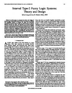
Figure 9. Input of IT2FLC membership function for an error e(t) NB 1

IV.

3

0.7 0.6 0.5 0.4 0.3 0.2 0.1 0 -5

-4

-3

-2 -1 0 1 2 Input Membership Function of de

3

4

5

Figure 10. Input of IT2FLC membership function for a change of the error Δe(t)

The membership functions and rule base parameters are the basic criteria that determine the performance of IT2FLC. Defining these parameters in line with the characteristics of the controlled system has a very essential to reach optimal performance should be considered in the design procedures of IT2FLC. The membership functions for the output error e(t), the change of the output error Δe(t) and gain feedback Kf consists of Negative Big (NB), Negative Small (NS), Zero (ZE), Positive Small (PS) and Positive Big (PB) fuzzy sets. To determine the IT2FLC rules, error e(t) and change of the error

7

IJEERI, VOL.2, NO. 1, MAR 2013

ISSN 2301-6132

Δe(t) of the voltage output of the DC-DC zeta converter used as the input to the IT2FLC, while the fuzzy output is gain Kf used as a closed-loop control applied to the DC-DC zeta converter.

Figure 12. A block diagram of DC-DC zeta converter equipped with IT2FLC

3

-R

azv*dzv.s3 +(bzv*dzv+azv)s2 +(czv*dzv+bzv)s+czv a.s4 +b.s3 +c.s2 +d.s+e

iz

Gzv

NB

NS

ZE

PS

PB

1

1

e

Vref

e

e Kf

delta e

0.9

delta e

vc

1/Vm

ZetaD

d

adv*ddv.s3 +(bdv*ddv+adv)s2 +(cdv*ddv+bdv)s+cdv

Degree of Membership

avv*dvv.s3 +(bvv*dvv+avv)s2 +(cvv*dvv+bvv)s+cvv a.s4 +b.s3 +c.s2 +d.s+e Gvv

0.6

Figure 13. A DC-DC zeta converter equipped with IT2FLC in MATLAB

0.5

implementation

0.4

From figure 12 can be seen that the input variable of IT2FLC consist of error e(t) and change of the error Δe(t) concerning the output voltages of the converter.

0.3

0.1 0 -15

-10

-5 0 5 Output Membership Function of Kf

10

15

Figure 11. Output of IT2FLC membership function for a gain Kf

Membership functions of error e(t) and change of the error Δe(t) used as IT2FLC input shown in Figure 11 and 12, while the IT2FLC output membership functions shown in Figure 13. The type of membership function for these sets is use a triangular form because the parametric functional description of triangular membership functions are the most economic one, the simplest and the most efficient form for many applications. The IT2FLC rules are identical with the type-1 FLC rules. The rules were designed to be used to improve the settling time and the overshoot, also minimize the minimum ITAE value of the dynamic response of the DC-DC zeta converter as shown in Table 3. A general rule base with 25 rules is framed with the help of IF AND THEN rules. In this paper, the IT2FLC method compared with a FLC and a PI controller method. A block diagram of small-signal linear model of the DCDC zeta converter equipped with IT2FLC is shown in Figure 9, while a block diagram of the converter using MATLAB software is shown in Figure 13. TABLE III.

IT2FLC RULES FOR DC-DC ZETA CONVERTER

Δe e NB NS ZE PS PB

ref

D*R

Vg

0.2

v (t )

2

z

0.7

Vo

Gdv

1

0.8

1

a.s4 +b.s3 +c.s2 +d.s+e

Modulator

IT2FLC

e(t )  v (t)  v (t) ref

0

e(t )  e(t )  e(t 1)

NB

NS

ZE

PS

PB

NB NB NS ZE PS

NB NS ZE PS PS

NS ZE PS PS PB

ZE PS PS PB PB

PS PS PB PB PB

vc (t)

d (t )

v0 (t)

 2013 IJEERI

e (t )  Vref (t )  V0 (t )

(25)

e(t )  e(t )  e(t  1)

(26)

where Vref(t) is the amplitude of reference output voltage at the tth sampling instant and e(t-1) is the amplitude of output voltage error at the (k-1)th sampling instant. The integral of absolute error (IAE), the integral of squared-error (ISE) or the integral of time-weighted-squarederror (ITSE) is a performance index criterion used to design a controller on the system. The three performance index criterions have the advantage and the disadvantage. The disadvantage of the IAE and the ISE is indices that they can produce a response with a relatively small overshoot but the settling time longer because they weigh all errors equally independent of time. Although the ITSE performance criterion can overcome the disadvantage of the ISE criterion but it can’t be sure to have the desired stability limit [17]. The IAE, ISE, and ITSE performance index criterion formulas are defined as follow,

tsim tsim IAE   r (t )  y (t ) dt   e(t ) dt t0 t0 tsim 2 ISE   e (t ) dt t0 tsim 2 ITSE   te (t )dt t0

(27) (28) (29)

The performance index criterion which is very popular used to control system design called the integral of time multiply by absolute error (ITAE) index. In this paper, the ITAE performance index criterion in the time domain is proposed for evaluating the proposed method. The ITAE performance index criterion is defined as follow,

8

IJEERI, VOL.2, NO. 1, MAR 2013

ISSN 2301-6132

tsim tsim ITAE   te(t ) dt   t (vref  v0 ) dt t0 t0

The output voltage of DC-DC zeta converter 25

(30)

20

Voltage(v)

where tsim is the time of integration B. Result Analysis 1. Case Study I The first part of the simulations in this paper is as follow, The input voltage VG of the DC-DC zeta converter is 15V, the desired output voltage is 5V and the load R is 1Ω. The result of the simulation for this case study is illustrated in Figures 14. The overshoot, settling time and ITAE data of the dynamic response of the DC-DC zeta converter from Figure 14 are shown in Table 4.

15

10

5

0

PI FLC IT2FLC 0

0.5

1

1.5

2 2.5 3 Time(second)

3.5

4

4.5

5 -4

x 10

Figure 15. The output voltage of the DC-DC zeta converter

The output voltage of DC-DC zeta converter 7

The overshoot, settling time and ITAE data of the dynamic response of the DC-DC zeta converter from Figure 15 are shown in Table 5.

PI FLC IT2FLC

6

Voltage(v)

5

4

TABLE V.

3

PI FLC IT2FLC

2

OVERSHOOT (V), SETTLING TIME (S, AND ITAE Overshoot(v) Settling time (s) ITAE 24.07 1.906e-04 2.6981e-06 22.70 1.436e-04 1.3042e-07 21.36 6.132e-05 1.2471e-08

1

0 0

0.5

1

1.5

2 2.5 3 Time(second)

3.5

4

4.5

5 -4

x 10

Figure 14. The output voltage of the DC-DC zeta converter TABLE IV. PI FLC IT2FLC

OVERSHOOT (V), SETTLING TIME (S), AND ITAE Overshoot(v) Settling time (s) ITAE 6.162 2.351e-04 3.9475e-06 5.493 1.810e-04 2.4866e-07 5.403 7.389e-05 3.5272e-08

From Figure 14 and Table 4 can be concluded that the proposed IT2FLC has more robust stability than the FLC and the PI controller applied to the DC-DC zeta converter.

From Figure 15 and Table 5 can be indicated that the proposed IT2FLC able to eliminate overshoots faster, achieves the smallest overshoot and also have the smallest ITAE value among all presented controllers applied to the DC-DC zeta converter. 3.

Case Study III In this case study, the input voltage VG of the DC-DC zeta converter is 20V, the desired output voltage is 5V and the load R is 5Ω. The result of the simulation is described in Figures 16. The output voltage of DC-DC zeta converter 7 PI FLC IT2FLC

6

Case Study II In this simulation, the input voltage VG of the DC-DC zeta converter is 15V, the desired output voltage is 20V and the load R is 1Ω. The result of the simulation is shown in Figures 15.

Voltage(v)

5

2.

4

3

2

1

0 0

0.5

1

1.5

2 2.5 3 Time(second)

3.5

4

4.5

5 -4

x 10

Figure 16. The output voltage of the DC-DC zeta converter

 2013 IJEERI

9

IJEERI, VOL.2, NO. 1, MAR 2013

ISSN 2301-6132

TABLE VI. OVERSHOOT (V), SETTLING TIME (S, AND ITAE Overshoot(v) Settling time (s) ITAE 6.187 1.939e-04 2.6001e-06 PI 5.520 1.531e-04 1.9943e-07 FLC IT2FLC 5.340 1.232e-04 1.2528e-08

50

40

30

20

10

0

Case Study IV In this case study, the input voltage VG of the DC-DC zeta converter is 20V, the desired output voltage is 30V and the load R is 5Ω. The result of the simulation is illustrated in Figures 17. The overshoot, settling time and ITAE data of the dynamic response of the DC-DC zeta converter from Figure 16 are shown in Table 7. From Figure 17 and Table 7 can be indicated that the proposed IT2FLC has robustness better than the other method i.e the FLC and the PI controller method. 4.

The output voltage of DC-DC zeta converter 40 PI FLC IT2FLC

35 30

Voltage(v)

25

0

0.5

1

15 10 5

0

0.5

1

1.5

2 2.5 3 Time(second)

3.5

4

4.5

5 -4

x 10

Figure 17. The output voltage of the DC-DC zeta converter TABLE VII. OVERSHOOT (V), SETTLING TIME (S, AND ITAE Overshoot(v) Settling time (s) ITAE 36.33 2.244e-04 1.3304e-05 PI 33.96 9.528e-05 1.4382e-06 FLC IT2FLC 31.65 6.040e-05 2.4034e-07

Case Study V In this part, the input voltage VG of the DC-DC zeta converter is 20V, the desired output voltage is 50V and the load R is 500Ω. The result of the simulation is shown in Figures 18. The overshoot, the settling time and the ITAE data of the dynamic response of the DC-DC zeta converter from Figure 16 are shown in Table 8. 5.

 2013 IJEERI

1.5

2 2.5 3 Time(second)

3.5

4

4.5

5 -4

x 10

Figure 18. The output voltage of the DC-DC zeta converter TABLE VIII. OVERSHOOT (V), SETTLING TIME (S, AND ITAE Overshoot(v) Settling time (s) ITAE 60.13 1.816e-04 2.5527e-05 PI 56.96 8.210e-05 3.3557e-06 FLC IT2FLC 52.78 5.865e-05 3.8077e-07

From Figure 18 and Table 8 can be indicated that the IT2FLC method have better performance than the FLC and the PI controller applied to the DC-DC zeta converter. The parameters of PI controller used as closed loop control design for all simulation in this paper are shown in Table 19. TABLE IX. Gain Kp Ki

20

0

PI FLC IT2FLC

60

Voltage(v)

The overshoot, settling time and ITAE data of the dynamic response of the DC-DC zeta converter from Figure 16 are shown in Table 6. From Figure 16 and Table 6 can be seen that the proposed IT2FLC provide damping better than the FLC and the PI controller method.

The output voltage of DC-DC zeta converter 70

THE VALUE OF PI CONTROLLER

Values 5 15

From all the simulation results that have been done either DC-DC zeta converter operates in step down or step-up mode can be seen that the proposed method was indeed more efficient and robust with less overshoot, faster settling time and have minimum ITAE value than the FLC and the PI controller. CONCLUSION

A novel closed-loop control design based on IT2FLC method for small-signal linear models of DC-DC zeta converter has been presented in this paper. An IT2FLC was used to handle the rule uncertainties when the operation is extremely uncertain and/or the membership grades can’t be exactly determined. A comparison between a PI controller, a FLC and an IT2FLC was performed. From the simulation results can be indicated that the IT2FLC method provide a better response and more robust against input voltage, output voltage and load resistance variations than the other methods i.e. FLC and PI controller. For further research development, PV modules can be used as the input voltage of DC-DC zeta converter and the other hybrid artificial intelligence algorithms also can be used to optimize the IT2FLC in order to provide more optimum results.

10

IJEERI, VOL.2, NO. 1, MAR 2013

ISSN 2301-6132

ACKNOWLEDGMENT The author would like highly acknowledge gratitude to Indonesian Government especially the Directorate General of Higher Education (DIRJEN-DIKTI) for the Excellency Scholarship (Beasiswa Unggulan) was awarded to the first author during his study at the Graduate Program, Department of Electrical Engineering, Institut Teknologi Sepuluh Nopember (ITS), Surabaya, Indonesia. The author also is very grateful to Conversion Energy Laboratory for all facilities provided during this research. Last but not least, the author would like to thank the anonymous reviewers for their insightful suggestions. REFERENCES [1] [2]

[3] [4]

[5] [6]

[7]

[8]

[9]

D. W. Hart, Introduction to Power Electronics, Prentice Hall, Inc., 1997. V. Vorperian, "Simplified Analysis of PWM Converters using Model of PWM Switch, Part I and Part II: Discontinuous Conduction Mode," IEEE trans. on Aerosp. Electron. Syst. , July 1990. R. W. Erickson and D. Maksimovix, Fundamental of Power Electronic. 2nd edition, Kluwer Academic Publisher, 2001. E. Vuthchhayt, C. Bunlaksananusornl, and H.Hirata, ”Dynamic Modeling and Control of a Zeta Converter”, International Symposium on Communications and Information Technologies (ISCIT), 2008, DOI : 10.1109/ISCIT.2008.4700242. T. J. Ross, Fuzzy Logic with Engineering Applications, 2nd ed. NewYork: Wiley, 2004. M. Ashari, T. Hiyama, M. Pujiantara, H. Suryoatmojo and M. H. Purnomo, “A Novel Dynamic Voltage Restorer with Outage Handling Capability Using Fuzzy Logic Controller”, The 2nd International Conference on Innovative Computing, Information and Control (ICICIC), 2007, DOI : 10.1109/ICICIC.2007.62. Zaheeruddin and V.K. Jain, ”A Fuzzy Expert System for Noise-Induced Sleep Disturbance”, Expert Systems with Applications, Vol.30, pp.761771, Sciencedirect Publisher, 2006. Ricardo Martínez, Oscar Castillo and Luis T. Aguilar,”Optimization of Interval Type-2 Fuzzy Logic Controllers for a Perturbed Autonomous Wheeled Mobile Robot using Genetic Algorithms”, Information Sciences, Vol.179, pp.2158–2174, 2009 Julio Romero Agüero and Alberto Vargas, “Calculating Functions of Interval Type-2 Fuzzy Numbers for Fault Current Analysis”, IEEE Transactions on Fuzzy Systems, Vol. 15, No. 1, February, 2007.

 2013 IJEERI

[10] Imam Robandi and Bedy Kharisma, “Design of Interval Type-2 Fuzzy Logic Based Power System Stabilizer”, International Journal of World Academy of Science, Engineering, and Technology, 2008. [11] A. Soeprijanto and M. Abdillah, “Type 2 Fuzzy Adaptive Binary Particle Swarm Optimization for Optimal Placement and Sizing of Distributed Generation”, The 2nd International Conference on Instrumentation, Communications, Information Technology and Biomedical Engineering (ICICI-BME), 2011, DOI : 10.1109/ICICIBME.2011.6108646. [12] Margo Pujiantara and Muhammad Abdillah, “Directional Over Current Relays (DOCRs) Coordination by Interval Type 2 Fuzzy Adaptive Particle Swarm Optimization (IT2FAPSO)”, International Journal of Academic Research (IJAR), Vol. 4. No. 3. May, 2012. [13] L.A.Zadeh,”The Concept of a Linguistic Variable and Its Application to Approximate Reasoning-1,”Information Science, vol.8, pp.199-249. [14] Qilian Liang and Jerry M. Mendel, “Interval Type-2 Fuzzy Logic System Theory and Design”, IEEE, October, 2000. [15] Jerry M. Mendel and Robert I.Bob John, “Type-2 Fuzzy Sets Made Simple”, IEEE, April, 2002. [16] Jerry M. Mendel and Feilong Liu, “Super-Exponential Convergence of The Karnik–Mendel algorithms for computing the centroid of an interval type-2 fuzzy set”, IEEE, April 2007. [17] R. A. Krohling, H. Jaschek, and J. P. Rey,“Designing PI/PID Controller for a Motion Control System Based on Genetic Algorithm,”in Proc. 12th IEEE Int. Symp. Intell. Contr., Istanbul, Turkey, July 1997, pp. 125– 130.

Muhammad Abdillah received the Sarjana Teknik (equivalent with B.Eng) degree from Department of Electrical Engineering, Institut Teknologi Sepuluh Nopember (ITS), Indonesia, 2009. Currently, he is pursuing M.Eng degree at the same Institute with Graduate Student Scholarship Award of The Excellency Scholarship (Beasiswa Unggulan) from The Directorate General of Higher Education (DIRJEN-DIKTI), Indonesia Government. During his undergraduate thesis research, he was a member of the section of the Power System Operation and Control (PSOC), Power System Simulation Laboratory. Since 2010, he has been with Power System Simulation Laboratory, as junior researcher. As author and co-author he has published 6 research papers at International Journals which indexed by Thomson and Scopus, 2 research papers at National Journals, 25 research papers at National Conferences, and 14 research papers at International Conferences. Currently, He is taking machine learning and quantum computing application used as design of wide area control system on power system for his graduate thesis research. His research interest includes power system operation and control, computational intelligence application on power system, power system stability, intelligent control and system, wide area monitoring, protection and control, data mining, machine learning, and quantum computing.

11