Design of an Optimal Trajectory Generator for a ...

Ecole Centrale de Nantes

Warsaw University of Technology

Master Erasmus Mundus EMARO “EUROPEAN MASTER ON ADVANCED ROBOTICS”

2010/2011

Final Master Thesis Report

Presented by: Cornelius Johannes Barnard On 19/07/2011

Title

Optimal Trajectory Generation for a High Speed Parallel Robot

Jury Evaluators: Sébastien Briot Stéphane Caro Wisama Khalil Ina Taralova Damien Chablat Janusz Fraczek

Researcher, IRCCyN, CNRS Researcher, IRCCyN, CNRS University Professor at ECN Researcher, IRCCyN, CNRS Researcher, IRCCyN, CNRS Professor, Warsaw University of Technology

Supervisor(s): Sébastien Briot and Stéphane Caro Laboratory: Institut de Recherche en Communications et Cybernétique de Nantes

Contents Title . . . . . . . . . . . . . . . . . . . . . . . . . . . . . . . . . . . . . . . . . . . . . .

0

List of Figures

iii

List of Tables

v

1 Introduction 1.1 Parallel Robots . . . . . . . . . . . . . . . . . . . . . . . . . . . . . . . . . . . . . 1.2 IRSBot2 . . . . . . . . . . . . . . . . . . . . . . . . . . . . . . . . . . . . . . . . .

1 3 4

2 Modeling 2.1 Elastodynamic Modeling . . . . . . . . . . . . 2.1.1 Lagrangian Formulation . . . . . . . . 2.1.2 Elastodynamic Modeling . . . . . . . . 2.1.3 Chosen Formulation: Assumed Modes 2.1.4 Inertia Matrix . . . . . . . . . . . . . 2.1.5 Stiffness Matrix . . . . . . . . . . . . . 2.1.6 Equations of Motion . . . . . . . . . . 2.1.7 Closed Form Dynamic Models . . . . . 2.1.8 Direct Dynamic Model . . . . . . . . . 2.1.9 Inverse Dynamic Model . . . . . . . . 2.1.10 Five Bar Mechanism Model . . . . . . 2.2 Geometric and Kinematic Modeling . . . . . 2.2.1 Rigid Inverse Geometric Model . . . . 2.2.2 Elastic Inverse Geometric Model . . . 2.2.3 Rigid Kinematic Model . . . . . . . . 2.2.4 Elastic Kinematic Model . . . . . . . . 2.3 Model Verification . . . . . . . . . . . . . . . 2.3.1 Modified Inertia Matrix . . . . . . . . 2.3.2 Frequency Analysis . . . . . . . . . . . 2.3.3 Deformation Analysis . . . . . . . . .

. . . . . . . . . . . . . . . . . . . .

. . . . . . . . . . . . . . . . . . . .

. . . . . . . . . . . . . . . . . . . .

. . . . . . . . . . . . . . . . . . . .

. . . . . . . . . . . . . . . . . . . .

. . . . . . . . . . . . . . . . . . . .

. . . . . . . . . . . . . . . . . . . .

. . . . . . . . . . . . . . . . . . . .

. . . . . . . . . . . . . . . . . . . .

. . . . . . . . . . . . . . . . . . . .

. . . . . . . . . . . . . . . . . . . .

. . . . . . . . . . . . . . . . . . . .

. . . . . . . . . . . . . . . . . . . .

. . . . . . . . . . . . . . . . . . . .

. . . . . . . . . . . . . . . . . . . .

. . . . . . . . . . . . . . . . . . . .

. . . . . . . . . . . . . . . . . . . .

. . . . . . . . . . . . . . . . . . . .

. . . . . . . . . . . . . . . . . . . .

. . . . . . . . . . . . . . . . . . . .

7 7 7 8 9 11 12 13 16 18 19 20 21 21 23 26 28 32 32 33 38

3 Trajectory Design 3.1 Geometric Path . . . . . . . . . . . 3.1.1 Clothoids . . . . . . . . . . 3.1.2 Lamé Curves . . . . . . . . 3.1.3 Polar Polynomials . . . . . 3.1.4 Geometric Path Discussion 3.2 Motion Profiles . . . . . . . . . . . 3.2.1 Seventh Degree Polynomial 3.2.2 Trapezoidal Profile . . . . . 3.2.3 Bang-bang Profile . . . . .

. . . . . . . . .

. . . . . . . . .

. . . . . . . . .

. . . . . . . . .

. . . . . . . . .

. . . . . . . . .

. . . . . . . . .

. . . . . . . . .

. . . . . . . . .

. . . . . . . . .

. . . . . . . . .

. . . . . . . . .

. . . . . . . . .

. . . . . . . . .

. . . . . . . . .

. . . . . . . . .

. . . . . . . . .

. . . . . . . . .

. . . . . . . . .

. . . . . . . . .

40 41 41 44 44 45 46 46 47 48

. . . . . . . . .

. . . . . . . . .

. . . . . . . . .

. . . . . . . . .

. . . . . . . . .

. . . . . . . . .

CONTENTS

3.3

CONTENTS

Trajectory Characteristics . . . . . . . . . . . . . . . . . . . . . . . . . . . . . . .

4 Simulation 4.1 Simulation Set 1 . . . . . . 4.1.1 Vibrational Domain 4.1.2 Simulation Results . 4.2 Simulation Set 2 . . . . . . 4.2.1 Vibrational Domain 4.2.2 Simulation Results . 4.3 Simulation Set 3 . . . . . . 4.4 Simulation Set 4 . . . . . .

. . . . . . . .

. . . . . . . .

. . . . . . . .

. . . . . . . .

. . . . . . . .

. . . . . . . .

. . . . . . . .

. . . . . . . .

. . . . . . . .

. . . . . . . .

. . . . . . . .

. . . . . . . .

. . . . . . . .

. . . . . . . .

. . . . . . . .

. . . . . . . .

. . . . . . . .

. . . . . . . .

. . . . . . . .

. . . . . . . .

. . . . . . . .

. . . . . . . .

. . . . . . . .

. . . . . . . .

. . . . . . . .

. . . . . . . .

. . . . . . . .

. . . . . . . .

. . . . . . . .

. . . . . . . .

49 55 56 56 56 62 62 63 68 70

5 Conclusion

72

Bibliography

74

ii

List of Figures 1.1 1.2 1.3 1.4

Pick-and-place operation for the packaging of healthcare Contemporary parallel robots . . . . . . . . . . . . . . . Schematic of IRSBot2 leg . . . . . . . . . . . . . . . . . . Planar five bar mechanism . . . . . . . . . . . . . . . . .

2.1 2.2 2.3 2.4 2.5 2.6 2.7 2.8 2.9 2.10 2.11 2.12 2.13 2.14

. . . .

. . . .

3 4 5 6

Generalized coordinates for each beam, qe = [qex qey ]T . . . . . . Mode shapes in bending and tension-compression . . . . . . . . . . . Schematic of the simulated system . . . . . . . . . . . . . . . . . . . Rigid Geometric Model . . . . . . . . . . . . . . . . . . . . . . . . . Superposition of rigid and elastic motions for clamped-free boundary Elastic Geometric Model . . . . . . . . . . . . . . . . . . . . . . . . . Elastic geometric model for leg i . . . . . . . . . . . . . . . . . . . . Configurations for natural frequency verification . . . . . . . . . . . The first three modes shapes as per CASTEM at position [0.35, 0.3] Contour plot of first natural frequency in workspace . . . . . . . . . Contour plot of second natural frequency in workspace . . . . . . . . Contour plot of third natural frequency in workspace . . . . . . . . . First natural frequency in workspace as a function of tool mass . . . Configurations for deformation verification . . . . . . . . . . . . . . .

. . . . . . . . . . . . . . . . . . . . . . . . conditions . . . . . . . . . . . . . . . . . . . . . . . . . . . . . . . . . . . . . . . . . . . . . . . . . . . . . .

. . . . . . . . . . . . . .

8 10 20 22 23 24 28 33 33 35 35 36 37 38

3.1 3.2 3.3 3.4 3.5 3.6 3.7 3.8 3.9 3.10 3.11 3.12 3.13 3.14 3.15 3.16

Pick-and-place trajectory. . . . . . . . . . . . . . . . . . . . . Adept half cycle using a Lamé curve . . . . . . . . . . . . . . Symmetric blending ray diagram . . . . . . . . . . . . . . . . Un-symmetric blending ray diagram . . . . . . . . . . . . . . Blending sections for the adept cycle . . . . . . . . . . . . . . Extended clothoid and Lamé curve generated for e = 44.5mm Motion profiles generated for tf = 1 . . . . . . . . . . . . . . Lamé curve trajectories . . . . . . . . . . . . . . . . . . . . . Clothoid pair trajectories . . . . . . . . . . . . . . . . . . . . Polar polynomial trajectories . . . . . . . . . . . . . . . . . . Lame curve joint space trajectory and spectral content . . . . Clothoid pair joint space trajectory and spectral content . . . Polar polynomial joint space trajectory and spectral content . Spectral content for the various geometric paths . . . . . . . Trajectory spectral content for various cycle times . . . . . . Trajectory spectral content for various blending lengths . . .

. . . . . . . . . . . . . . . .

. . . . . . . . . . . . . . . .

40 41 42 43 45 46 48 50 50 50 51 52 52 53 53 54

4.1 4.2

Position of the trajectory in the workspace (gravity is taken upwards) . . . . Frequency distribution along Adept Cycle with a 100g payload. Line styles: Lamé, - - Clothoid, ... Polar . . . . . . . . . . . . . . . . . . . . . . . . . . . . Simulation results for a 100g payload in the task space . . . . . . . . . . . . .

. . . . . .

55

4.3

products . . . . . . . . . . . . . . . . . .

. . . . . . . . . . . . . . . .

. . . . . . . . . . . . . . . .

. . . . . . . . . . . . . . . .

. . . .

. . . . . . . . . . . . . . . .

. . . .

. . . .

. . . . . . . . . . . . . . . .

. . . .

. . . . . . . . . . . . . . . .

. . . .

. . . . . . . . . . . . . . . .

. . . .

. . . . . . . . . . . . . . . .

. . . . . . . . . . . . . . . .

56 57

LIST OF FIGURES

4.4 4.5 4.6 4.7 4.8 4.9 4.10 4.11 4.12 4.13 4.14 4.15 4.16 4.17 4.18

LIST OF FIGURES

Joint torques for a 100g payload. Line styles: - Lamé, - - Clothoid, ... Polar . . . Elastic Coordinates in Bending for a 100g payload. Line styles: - Lamé, - Clothoid, ... Polar . . . . . . . . . . . . . . . . . . . . . . . . . . . . . . . . . . . Elastic Coordinates in Tension-Compression for a 100g payload. Line styles: Lamé, - - Clothoid, ... Polar . . . . . . . . . . . . . . . . . . . . . . . . . . . . . . Spectral Distribution for a 100g payload. Line styles: - Lamé, - - Clothoid, ... Polar Error norm in the task space with a 100g payload. Line styles: - Lamé, - Clothoid, ... Polar . . . . . . . . . . . . . . . . . . . . . . . . . . . . . . . . . . . Frequency distribution along Adept Cycle with a 6000g payload. Line styles: Lamé, - - Clothoid, ... Polar . . . . . . . . . . . . . . . . . . . . . . . . . . . . . . Simulation results for a 6kg payload in the task space . . . . . . . . . . . . . . . Joint torques for a 6000g payload. Line styles: - Lamé, - - Clothoid, ... Polar . . Elastic Coordinates in Bending for with a 6kg payload. Line styles: - Lamé, - Clothoid, ... Polar . . . . . . . . . . . . . . . . . . . . . . . . . . . . . . . . . . . Elastic Coordinates in Tension-Compression for a 6000g payload. Line styles: Lamé, - - Clothoid, ... Polar . . . . . . . . . . . . . . . . . . . . . . . . . . . . . . Spectral Distribution for a 6kg payload. Line styles: - Lamé, - - Clothoid, ... Polar Error norm in the task space with a 6kg payload. Line styles: - Lamé, - - Clothoid, ... Polar . . . . . . . . . . . . . . . . . . . . . . . . . . . . . . . . . . . . . . . . . Task space position for a payload of 6kg and tf = 0.215ms Line styles: - Lamé, - Clothoid, ... Polar . . . . . . . . . . . . . . . . . . . . . . . . . . . . . . . . . . Task space velocity and acceleration for a payload of 6kg and tf = 0.215s Line styles: - Lamé, - - Clothoid, ... Polar . . . . . . . . . . . . . . . . . . . . . . . . . Varying blending lengths for a 6000g payload. Line styles: - Lamé, - - Clothoid, ... Polar . . . . . . . . . . . . . . . . . . . . . . . . . . . . . . . . . . . . . . . . .

iv

58 58 59 59 61 62 63 64 65 65 66 67 68 68 70

List of Tables 2.1 2.2 2.3 2.4 2.5 2.6

Modal parameters for bending deformation . . . . . . . . Parameters of the modeled five bar mechanism . . . . . . Natural Frequencies at Various Robot Configurations . . . Third natural frequency with adjusted inertia in the FEA Deformation under Fx = 100N . . . . . . . . . . . . . . . Deformation under Fy = 100N . . . . . . . . . . . . . . .

. . . . . .

. . . . . .

. . . . . .

. . . . . .

. . . . . .

10 20 34 34 39 39

3.1 3.2 3.3 3.4 3.5

Blending lengths for geometric paths . . . . . . . . . . . . . . . . . . . . . Boundary conditions for the 7th degree polynomial . . . . . . . . . . . . . Tested motion profiles and geometric paths . . . . . . . . . . . . . . . . . Task space velocity and acceleration comparison of generated trajectories Characteristic features of joint space trajectories . . . . . . . . . . . . . .

. . . . .

. . . . .

. . . . .

. . . . .

45 46 49 49 51

4.1 4.2 4.3

Adept cycle times and payloads . . . . . . . . . . . . . . . . . . . . . . . . . . . . Terminal end-effector state at tf = 0.3 for a payload of 100g . . . . . . . . . . . . Maximum task space velocity and acceleration for a payload of 100g and a cycle time of tf = 0.3s . . . . . . . . . . . . . . . . . . . . . . . . . . . . . . . . . . . . Task space velocity and acceleration comparison of generated trajectories . . . . Residual norms at end effector end points . . . . . . . . . . . . . . . . . . . . . . Averaged terminal end-effector state at tf = 0.43 for a payload of 6000g . . . . . Maximum task space velocity and acceleration for a payload of 6kg and a cycle time of tf = 0.43 . . . . . . . . . . . . . . . . . . . . . . . . . . . . . . . . . . . . Task space velocity and acceleration comparison of generated trajectories . . . . Residual error norms at end effector end points for a payload of 6kg . . . . . . . Comparison of results for a cycle time of tf = 0.215s . . . . . . . . . . . . . . . . Residual error norms at end effector end points for a payload of 6kg . . . . . . . Comparison of short and extended cycle lengths . . . . . . . . . . . . . . . . . . . Comparison of error norms on short and extended cycle lengths . . . . . . . . . .

55 57

4.4 4.5 4.6 4.7 4.8 4.9 4.10 4.11 4.12 4.13

. . . . . .

. . . . . .

. . . . . .

. . . . . .

. . . . . .

. . . . . .

. . . . . .

. . . . . .

57 60 62 63 63 66 67 69 69 71 71

Chapter 1

Introduction The advantages of parallel robots over serial robots for high speed applications is a subject which is drawing much attention of late. Currently parallel robots are finding more and more acceptance in high-speed pick-and-place operations. Parallel robots significantly improve the throughput of many robotic tasks [3, 21]. The drive for higher operational speeds and higher payload-to-weight ratios is shifting the design of manipulators to more lightweight structures [25]. In contrast to serial manipulators, parallel robots offer a lower mass-to-inertia ratio and a higher stiffness-to-mass ratio1 [20]. These benefits come at the price of increased modeling and design complexity. The design of parallel robots is accompanied with several closed kinematic chains with inherent kinematic constraints. As for all high-speed mechanisms, vibratory phenomena appear that deteriorate the robot accuracy and its dynamic performance. The performance criteria on speed and accuracy have rendered classical rigid body dynamics for the description of the dynamic behaviour of such systems inadequate [22]. Due to the inherent flexibility of these lightweight structures, inertial forces result in unwanted structural vibration [28]. These vibrations deteriorate not only the accuracy and performance of the manipulator but also cause significant wear and tear on the components [15].

1

Structural Rigidity

Chapter 1. Introduction

Problem Statement The IRCCyN2 robotics team has recently proposed a new high speed parallel manipulator, IRSBot2, with two degrees of freedom. Investigate the use of an optimal motion generator for the reduction of vibrations in IRSBot2 by carefully planning the displacements of the end effector. The optimality of this motion generator is concerned with the level of vibration reduction and the speed at which the pick-and-place operation is conducted. The scope of this thesis is as follows: • Development of an elastodynamic model of the IRSBot2 • Design of a motion generator: – The definition of the geometric path as based on the Adept Cycle – The definition of the motion profile or temporal control law • Spectral analysis of the control law and manipulator response to verify that the natural modes of vibration are not excited This bibliographic report consolidated recent work done in vibration reduction, thereby providing a thorough foundation from which vibration in parallel manipulators can be managed in particular for pick-and-place tasks common in industry today. In accordance with the literature studied, this bibliographic work was divided into three chapters concerning: 1. Elastodynamic Modeling 2. Trajectory Design 3. Control The thesis work limits the scope of the material identified in the bibliographic report and in this masters dissertation, the work is divided as follows: 1. Geometric and Kinematic Modeling 2. Elastodynamic Modeling 3. Trajectory Design 4. Simulation

2

Institut de Recherches en Communications et Cybernétique de Nantes

2

Chapter 1. Introduction

1.1

1.1 Parallel Robots

Parallel Robots

Before expanding on the above mentioned areas, a brief introduction to parallel robots is provided. Particularities relevant to this work are highlighted. The master thesis of Germain [10] provides a comprehensive overview of parallel robots used for pick-and-place tasks in industry today. Pick-and-place operations comprise both primary handling and case packing (see figure 1.1)[18]. These operations usually require between 2 and 4 degrees of freedom (DOF) - typically two or three translational degrees of freedom and if required, one rotational degree of freedom [10, 11, 9].

Figure 1.1: Pick-and-place operation for the packaging of healthcare products [19].

Several four degree of freedom parallel robots exist on the market today. Robots with 3 translational degrees of freedom and one rotational degree of freedom about the z-axis are capable of performing Schönflies motions. Adept Technology [13] currently have the fastest pick-and-place robot, the Quattro (number 1 in figure 1.2) in production. The Quattro is capable of performing up to 240 cycles per minute 3 . Figure 1.2 also shows the Flex-picker delta robot from ABB (2) and the McGill SMG robot (3). For tasks requiring two degrees of freedom (DOF), such as the one considered for this thesis, simpler robots may be used [10]. Two degree of freedom robots are considered as planar robots and are used to position a point in the plane of operation. The Par2 (number 4 in figure 1.2) developed in the ANR4 100g Objective project and the Elau PacDrive D2 (5) [7] are examples of 2DOF designs. A key design requirement for these robots is to ensure structural rigidity perpendicular to the operation plane, thereby resisting forces normal to this plane. This requirement is for instance addressed by the second set of legs in the Par2 robot rendering it much stiffer than the PacDrive D2. Nonetheless, Germain [10] notes several drawbacks of the Par2: 3 4

Standard cycle: 25mm/350mm/25mm Agence Nationale de la Recherche

3

Chapter 1. Introduction

1.2 IRSBot2

Figure 1.2: Contemporary parallel robots [10].

1. It has a complex architecture. 2. The inclusion of stiff metallic belts for the prevention of lateral motion introduces undesired elasticity. 3. High tolerance requirements for its manufacturing and construction due to the number of joints. 4. The identification of its dynamic behaviour is difficult to obtain.

1.2

IRSBot2

The newly conceived IRSBot2 (see figure 1.3) responds to the aforementioned drawbacks. The IRSBot2 structure is of spatial architecture and offers certain advantages [10]: 1. It consists of only two legs, thereby reducing the overall mass and improving the dynamic behaviour of the system. 2. The design is such that a number of the links, rather than being subjected to bending, are only subjected to tensile, compression and torsional forces, also improving the dynamic performance of the design.

In figure 1.4, the global coordinate frame O, attached to the fixed base, is shown in plane P0 and the moving platform (always parallel to the base) is defined in plane P1 . Each leg consists of two distinct parts. The upper part, composed of links 0i , 1i , 2i , 3i forms a parallelogram. The lower part, of greater complexity, exists between links 3i and 7i . Note that the joint axes y1ji are always within plane P1 which, in turn is always parallel to planes P0 and P2 . Furthermore note that the axes y1ji and z2ji are orthogonal. The assembly of the lower part of the leg gives rise to the spatial movement particular to IRSBot2. The geometric description of the robot will briefly be discussed. For more detail the reader is directed to Germain [10].

4

Chapter 1. Introduction

1.2 IRSBot2

Figure 1.3: Schematic of IRSBot2 leg [10]

Loop Closure The loop closure equations are used to develop the inverse and geometric models. Germain [10] uses the parametrization shown in figure 1.4 with the definition of the virtual link l2eq to define the loop closure equations. The ± symbol designates + to leg 1 and − to leg 2:

Inverse Geometric Model The inverse geometric model (IGM) gives the joint positions, q1 and q2 , as a function of the Cartesian coordinates, x and z, of the end effector. As with other parallel manipulators, the loop closure equations allow the IGM to be easily expressed. The expression of the IGM is included as is from [10]. Here ± refers to the working modes:

5

Chapter 1. Introduction

1.2 IRSBot2

Direct Geometric Model The direct geometric model (DGM) is also derived from the loop closure equations and is presented as in Germain [10]. Here ± refers to the assembly modes of the robot:

Simplified Model As a preliminary study, the chosen model was simplified. The simplest parallel mechanism with revolute joints resembling the IRSBot2, is a planar five bar mechanism (figure 1.4)

Figure 1.4: Planar five bar mechanism [26]

In the next chapter (Chapter 2), firstly the rigid and elastic kinematics of the planar five bar mechanism will be developed. Secondly the elastodynamic modeling is developed from first principles and lastly, the resultant model is verified.

6

Chapter 2

Modeling 2.1

Elastodynamic Modeling

Elastodynamic modeling can be done using either a hybrid Newton Euler approach or a Lagrangian Formulation. The Lagrangian formulation is opted for, and is developed in the next section.

2.1.1

Lagrangian Formulation

The Lagrange equations are used to derive the elastodynamic model as it is readily applied to the analysis of closed loop structures. The Lagrangian formulation equates the nonconservative forces acting on the system to the change of energy in the system [1]. The Lagrangian L of a robot or manipulator is defined as the difference between the kinetic energy E and the potential energy U : L=E−U (2.1) The formulation of the constituent terms of the Lagrangian are shown in equations 2.2 and 2.3. Development of the inertia, M, and stiffness, K, matrices found in the kinetic and potential energy terms vary according to the elastodynamic modeling used. For beam j: Kinetic Energy : 1 Ej = q˙j T Mj q˙j 2

(2.2)

where Mj : is the symmetric positive definite inertia matrix of beam j 1 . qj : is the vector of generalized coordinates qj = [xAj , yAj , θj , qej ]T (see figure 2.1). Potential Energy 1 Vej = qj T Kj qj 2 where Kj : is the stiffness matrix of beam j

1

The inertia matrix is also referred to as the mass matrix

(2.3)

Chapter 2. Modeling

2.1 Elastodynamic Modeling

Figure 2.1: Generalized coordinates for each beam, qe = [qex

2.1.2

T

qey ]

Elastodynamic Modeling

The various elastodynamic modeling techniques used to develop the Lagrangian formulation are compared and contrasted next, with the motivation for the use of Assumed Modes is discussed in section 2.1.2. Finite Element Modeling This method represents each link as an assembly of a finite number of elements, wherein each element is a continuous member of the link [17]. Linear finite elements make use of polynomial interpolation functions (expressing nodal displacements) or assumed mode techniques to characterize a link’s elastic behaviour [5, 25]. Boundary conditions, changes in geometry and physical properties can be easily accounted for with the finite element method (FEM) [25]. Greater model accuracy is used by either using more elements or by using higher order elements [21]. Lumped Parameter Model Lumped parameter models or rigid finite element models [29], also referred to as the finite segment method by Shabana [24], describe manipulators as a set of interconnected rigid bodies [22]. The manipulator links are discretized into a series of rigid bodies which are then connected by linear springs thereby introducing flexible features to the model [25]. The method of lumped parameters is also referred to as the method of Virtual Joints or VJM [3] and is considered to be the simplest method to implement. In its standard formulation, the method does not lend itself well to closed loop robots. Briot, Pashkevich and Chablat [3] address the problem of passive joints in closed loop robots and propose a reduced method which decreases the dimension of the problem by using assumed mode techniques. Despite its simplicity, Theodore and Ghosal [25] indicate that the method is seldom used due to the difficulty of determining the spring constants. Pashkevich, Chablat and Wenger [20] do however propose a method of determining the virtual stiffness from a finite element link stiffness evaluation.

8

Chapter 2. Modeling

2.1 Elastodynamic Modeling

Assumed Modes The assumed mode method (AMM)2 describes flexible displacements by a truncated modal series, in terms of spatial mode eigen functions and time-varying mode amplitudes [6, 25]. The truncated modal series refers to a subgroup of trigonometric functions each depicting the physical modal behaviour of links or beams. The mode shapes can be found by solving the free vibration problem for a given set of boundary conditions. The mode shapes are characterized by their corresponding eigen vectors and occur at a frequency given by the associated eigen values [4]. If clamped-mass boundary conditions are chosen, time-varying mode amplitudes occur as the frequency equations are time dependent3 . Clampedfree boundary conditions are used for simplification purposes at the expense of overestimated natural frequencies. The AMM is modeled using the floating reference frame discussed in section 2.2.2 [28].

2.1.3

Chosen Formulation: Assumed Modes

Dwivedy and Eberhard [6] present an extensive review on various elastodynamic modeling approaches. The bibliographic report compared and contrasted the Assumed Modes Method, the Finite Element Method and Lumped Parameter Modeling. Based on the bibliographic survey, the Assumed Modes Method was chosen as the modeling approach. The supporting factors of this approach are [25]: • Assumed Modes is recommended for manipulators with flexible links of uniform crosssection • Well suited for numerical simulations The approach calls for the superposition of elastic motions on the rigid motions in the system [22, 28]. The properties of the Assumed Modes approach are listed next: • Flexible displacements are represented by truncated modal series [6, 25] • Floating reference frames are introduced to superpose the flexible deformations on the rigid positions of the distal end of each link [2, 5, 21, 24] • Beam deformations are described with appropriate shape functions Shape Functions The truncated modal series used to describe the deformation of a beam are referred to as the shape functions. For the planar case, bending and tension-compression deformations are considered. The shape functions, Φ are coupled with time varying elastic coordinates qe [6, 25]. In bending, these coordinates are perpendicular to the undeformed axial direction of the beam, whereas they are collinear with this axis in tension-compression deformation. The vector Φ is of size 1 × k, with k being the number of modes used for modeling. A two degree of freedom pick and place robot is typically actuated at its base. It is assumed that the actuated links are rigidly connected to these actuators, as such, these links are modeled as beams in bending [2]. For link j: 2

Also called the Rayleigh-Ritz approach [3, 21] The clamped-mass rather than the clamped-free boundary conditions are used to include the inertial effects of other links [25] 3

9

Chapter 2. Modeling

2.1 Elastodynamic Modeling

Clamped-free : φjk (ξ) = sin(αk lj ξ) + ak cos(αk lj ξ) − sinh(αk lj ξ) − ak cosh(αk lj ξ)

(2.4)

where ak and αk lj : are modal parameters for mode k [22] ξ=

x lj

: lj is length of link j and x is the position along the axial direction of the beam

The first three modal parameters are considered and are taken from Bouzgarrou et al [2]: Mode 1 2 3

ak -1.3622 -0.98186 -1.0008

αk lj 1.8751 4.6941 7.8548

Table 2.1: Modal parameters for bending deformation

The distal links are assumed to be pin-connected, and are thus only loaded in the axial direction. This loading corresponds to cases in which a beam experiences only tensile or compressive deformations: Pin Connected :

π φjk (ξ) = sin (2k − 1) ξ 2 



(2.5)

where ξ=

x lj

: lj is length of link j and x is the position along the axial direction of the beam

The normalized shape functions are shown in figure 2.2. Bending

2 1 0

0

0.2

0.4

0.6

0.8

1 0 −1 −2

1

4 Mode 3: phi3

2 Mode 2: phi2

Mode 1: phi1

3

0

0.2

0.4

ksi

0.6

0.8

2 0 −2

1

0

0.2

0.4

ksi

0.6

0.8

1

0.6

0.8

1

ksi

Tension−Compression

0.5

0

0

0.2

0.4

0.6 ksi

0.8

1

1 Mode 3: phi3

1 Mode 2: phi2

Mode 1: phi1

1

0.5 0 −0.5 −1

0

0.2

0.4

0.6

0.8

1

0.5 0 −0.5 −1

0

0.2

0.4

ksi

ksi

Figure 2.2: Mode shapes in bending and tension-compression

Having introduced the assumed modes method of modeling and the relevant shape functions, the inertial and stiffness matrices may now be developed.

10

Chapter 2. Modeling

2.1.4

2.1 Elastodynamic Modeling

Inertia Matrix

The inertia matrix, Mj , in equation 2.2 may now be developed. The kinetic energy of a elastic beam, j, may now expressed using the shape functions [2, 22, 5]: 1 E= 2

Z lj 0

r˙ TM r˙ M dx

(2.6)

The velocity vector, r˙ M , is defined according to the type of deformation modeled on the beam. rM describes the position of a point on a deformed beam in the global reference frame as follows: "

rM

#

"

#

"

#

x l ξ u (ξ, t) = Aj + R(θj ) j + R(θj ) xj yA j 0 uyj (ξ, t)

(2.7)

where xAj and yAj : Locate the base of link j R(θj ) : A rotation matrix which orientates the beam at an angle θj uxj (ξ, t) and uyj (ξ, t) : Are the deformations on the beam evaluated at position ξ at time t: uxj (ξ, t) = Φx (ξ)qexj (t) uyj (ξ, t) = Φy (ξ)qeyj (t) Deriving expression 2.7 with respect to time, the velocity of the point rM , for a beam in pure bending (deformation only being allowed in uyj (ξ, t), i.e. uxj (ξ, t) = 0) may be found: "

r˙ M =

1 0 −Φy qeyj 0 1 lj ξ

  ˙j # xA ˙ j 0   yA   ˙  Φy  θj 

(2.8)

qe˙yj

To obtain the mass matrix for a beam in pure bending, the following calculation, contained in 2.6, must be performed: 

1 Z 1 0  Mj = mj  −Φ  y qeyj 0 0



0 " 1   1 0 −Φy qeyj  lj ξ  0 1 lj ξ Φy

#

0 dξ Φy

(2.9)

This results in the following mass matrix, dimensioned according to the number of generalized coordinates:   1 0 −Φy qeyj 0 Z 1 0 1 lj ξ Φy    Mj = mj (2.10)   dξ T T 2  −q Φ l ξ (l ξ) l ξΦ eyj y j j j y  0 0 Φy T lj ξΦy T Φy T Φy Similarly the mass matrix of a beam in tension and compression may be found. Here, deformation is only allowed in uxj (ξ, t) and so uyj (ξ, t) = 0): "

r˙ M =

1 0 0 0 1 lj ξ + Φx qexj

  # x˙ Aj  Φx   y˙ Aj   ˙  0  θ 

q˙ exj

11

(2.11)

Chapter 2. Modeling

2.1 Elastodynamic Modeling

This results in the following mass matrix: 1 Z 1 0  Mj = mj  0  0 Φx T

0 1

0 lj ξ + Φx qexj 2 (lj ξ) + 2lj ξΦx qexj + qexj T Φx T Φx qexj 0

Φx 0    dξ 0  lj ξ + qexj T Φx T 0 Φx T Φx (2.12) Beams which experience both bending and tension-compression deformation (i.e. deformation is allowed in both uxj (ξ, t) and uyj (ξ, t)), are described as follows: 





"

r˙ M =

1 0 −Φy qeyj 0 1 lj ξ + Φx qexj



x˙ Aj  #  y˙  0  A˙ j   θj   Φy  q˙ e   xj  q˙ eyj

Φx 0

(2.13)

Resulting in the rather complicated mass matrix: 

1 0

0 1

0

lj ξ + qexj T Φx T 0 Φy T

 Z 1  −qe T Φy T Mj = mj yj  0  Φx T 

−Φy qeyj lj ξ + Φx qexj ∆ T −Φx Φy qeyj ΥT

Φx 0 0 Φy    −qeyj T Φy T Φx Υ   dξ  T Φx Φx 0  0 Φy T Φy (2.14) 

With, ∆ = (lj ξ)2 +qexj T Φx T Φx qexj +qeyj T Φy T Φy qeyj +2lj ξΦx qexj −2qeyj T Φy T Φx qexj −2lj ξΦy qeyj Υ = lj ξΦy + qexj T Φx T Φy

2.1.5

Stiffness Matrix

The stiffness matrix, Kj , in equation 2.2 is necessary for the evaluation of the elastic potential energy of a elastic beam. For beams in bending [25]: K yj

EIj = 3 lj

∂ 2 uy (ξ, t) ∂ξ 2

Z 1 0

!2

dξ

(2.15)

Considering the first 3 modes of deformation, the stiffness matrix of a beam in pure bending is expressed as the diagonal matrix Ky :

Kyj =

EIj lj3

   R 1 ∂ 2 φy1 (ξ) 2 dξ  0 ∂ξ 2     0   



0 R1



0

0

∂ 2 φy2 (ξ) ∂ξ 2

0 2

dξ

0 R1

0

0



∂ 2 φy3 (ξ) ∂ξ 2

2

dξ

       

(2.16)

Similarly for beams in tension and compression: Kxj

EAj = lj

 Z 1 ∂uy (ξ, t) 2

∂ξ

0

12

dξ

(2.17)

Chapter 2. Modeling

2.1 Elastodynamic Modeling

Thus, for the first three modes: R   1 ∂φx1 (ξ) 2 dξ 0 ∂ξ  EAj   K xj = 0 lj  

0

0

R 1  ∂φx2 (ξ) 2 0

∂ξ

0



dξ

0 R 1  ∂φx3 (ξ) 2

0

0

∂ξ

dξ

    

(2.18)

For beams which deform in both bending and tension-compression, the stiffness matrix K is augmented diagonally4 : # " Kxj 0 (2.19) Kj = 0 K yj

2.1.6

Equations of Motion

The dynamics of the complete system may be solved by creating the total inertia and stiffness matrices, Mtot and Ktot . The matrices are collected in diagonal matrices as follows: 



Mtot

M1 0 . . . 0  M2 . . . 0    0  = . .. ..  ..  . . . .   . 0 0 . . . Mn

(2.20)

and, 

Ktot

Ktot1   0 =  ..  .

0 Ktot2 .. .

0

0

... ... .. .

0 0 .. .

. . . Ktotn

     

(2.21)

Where, n : refers to the number of elastic beams in the system and, "

Ktotj

0 0 = 3×3 0 Kj

#

(2.22)

The Lagrangian formulation of the elastodynamic problem is developed from the Lagrangian defined in 2.1. For closed loop robots, the loop closure constraints are reflected in the formulation [28]:     d ∂L T ∂L F= − + ΨTq λ (2.23) dt ∂ q˙ ∂q Where, F : is the vector sum of nonconservative external forces. In the absence of external forces this is simply equal to the joint torques, Γ Ψ =

∂Ψ ∂q

is c × N matrix with c the number of constraints and N the number of parameters. Ψ = [CT BT AT ]T

λ : is a c × 1 vector of Lagrange multipliers q = [q1 , q2 , . . . , qn ]T , refers to the concatenation of the generalized coordinate vectors of each beam in the system 4

Attention must be paid to the ordering of the elastic terms in the generalized coordinate vector

13

Chapter 2. Modeling

2.1 Elastodynamic Modeling

The Ψ matrix is referred to as a Jacobian matrix in robotics literature and is responsible for the loop closure equations as discussed in section 2.2.4. It should be noted that the potential energy term, in the case of flexible manipulators, refers to both the gravitational potential energy and the elastic potential energy U = Vg + Ve [2, 22, 25]. The Lagrangian formulation 2.23 is now developed in a stepwise manner: Kinetic Energy First the time-velocity derivative term is analyzed. Note that a new inertia matrix, MR , is used. This matrix is appropriately oriented within the global reference frame as shown in equation 2.25. " #T   d ∂E T d ∂ 21 q˙ T MR q˙ = (2.24) dt ∂ q˙ dt ∂ q˙ with, MR = Rtot Mtot Rtot T where, 



Rtot

R1 0 . . . 0    0 R2 . . . 0   = . .. ..  ..  . . .   .. 0 0 . . . Rn

and, "

R(θj ) 0 Rj = 0 Ikj ×kj

#

(2.25)

where, θj : is the rotational term in the generalized coordinate vector qj kj : refers to the number of modes included on beam j The result of equation 2.24 may thus be expressed as follows: d ∂E dt ∂ q˙ 

T

˙ R q˙ = MR q ¨+M

(2.26)

with, T ˙ R=R ˙ tot Mtot Rtot T + Rtot M ˙ tot Rtot T + Rtot Mtot R ˙ tot M

As seen earlier, the inertia matrix Mtot is a function of the elastic coordinates qe , which, in ˙ tot term seen in equation 2.1.6. turn are time variant, thus the time derivative leads to the M Next the positional derivative term may be evaluated, this is done for each generalized coordinate h: ∂ 1 q˙ T MR q˙ 1 ∂E = 2 = q˙ T MRqh q˙ (2.27) ∂qh ∂qh 2 where, MRqh = Rqh MRT + RMqh RT + RMRqh T Collectively, the position derivative of beam j may be written: 

0 0



 

 ∂E     = MRqj =  1 T T T  q˙ Rθj Mj R + RMj Rθj q˙ j  ∂qj 2 j    1 T q ˙ RM R q ˙ q ej j 2 j

(3+kj )×1

where 14

(2.28)

Chapter 2. Modeling

2.1 Elastodynamic Modeling

kj : refers to the number of modes modeled on beam j "

− sin θ − cos θ Rθ = cos θ − sin θ

#

Elastic Potential Energy The elastic potential energy is not a function of q˙ and thus the time-velocity derivative term is zero. The position derivative term is left to be determined as follows, note that this term is in fact only related to the elastic coordinates qe due to the construction of Ktot in equation 2.21: ∂ 1 qKtot q ∂Ve = 2 = Ktot q ∂q ∂q

(2.29)

It can be seen that this term reduces the well known Hook’s law, relating an applied force to a corresponding elastic deformation. Gravitational Potential Energy Finally the gravitational potential energy may be assessed. The gravitational potential energy Vgj for beam j is determined at the beam mid-point using the mass mj of the link: Z

V gj =

m

−−−→ gT OM ∗ j dm = mj gT

Z 1 −−−→

OM ∗ j dξ

(2.30)

0

−−−→ with OM ∗ j : "

#

" #

#

"

lj −−→ x u (ξ, t) OM j = Aj + R 2 + R xj yA j uyj (ξ, t) 0

|

{z

}

−−→ OM j

|

{z

(2.31) }

−−−→ M M ∗j

with uxj = φxj (ξ)qexj , uyj = φyj (ξ)qeyj , and g = [0 − g]T , the term for the gravitational effects can be found from: l sin(θj ) + αqej ) 2 where, α: is a vector depending on θj . The gravitational efforts may be found from: Vgj = mj g(yAj +

Vgj = Qj T qj

(2.32)

(2.33)

Open Loop Lagrangian Formulation The terms developed in the preceding subsections may now be combined to form the open loop Lagrangian formulation, that is to say, that at this point in time, the closure constraints are ignored: F = MR q ¨+H (2.34) where the Coriolis and gravitational elements are included in the vector H: ˙ R q˙ − MRq − Ktot q − Q H=M




15

(2.35)

Chapter 2. Modeling

2.1 Elastodynamic Modeling

Ordering and regrouping of the Lagrangian Formulation It is desired to collect and reorder the elements in equation 2.34 according to the actuated, elastic and passive coordinates. This reordering allows the elastodynamic model to conform to the modeling used during the development of the kinematic relations of the system. The process of reordering may be explained as follows: • Identify all actuated coordinates, note their indexing and assign them to the vector qa • Identify all elastic coordinates, note their indexing and assign them to the vector qe • Identify all passive coordinates, note their indexing and assign them to the vector qp . If there are supplementary passive coordinates, such as the inclusion of lumped masses or inertias, their associated coordinates be appended to qp . The inclusion of these masses must be reflected on the diagonal of the mass matrix MR and must also be appended to the gravitational efforts Q5 • Identify all coordinates which are implicitly constrained. Eliminate the corresponding rows and columns from Mtot and eliminate the appropriate elements from the Coriolis and gravitational terms vector H. Implicitly constrained coordinates are coordinates which can, under no condition, experience any form of motion. For the five bar mechanism considered, the set of implicitly constrained generalized coordinates are the x and y base positions of the actuated links. The reordering allows the independent and dependent coordinates to be distinguished as qi = [qa , qe ]T and qd = qp . This gives rise to the generalized coordinate vector of the following form: "

q=

qi qd

#





qa   =  qe  qp

(2.36)

The open loop Lagrangian expression may thus be written with greater detail: 













Γa Maa Mae Map q ¨a Ha        Γ M M M q ¨ = +  e   ea  He  ee ep   e  Γp Mpa Mpe Mpp q ¨p Hp

2.1.7

(2.37)

Closed Form Dynamic Models

The closure constraints may be introduced into equation 2.37. This will allow the formulation of the inverse and direct dynamic models. These models are used as follows: • The inverse dynamic model, delivers the required actuator efforts τa and the resultant elastic deformations in acceleration, q ¨e , as a function of a desired trajectory in the actuated coordinates qa , q˙ a and q ¨a • The direct dynamic model, determines the resultant independent coordinate accelerations as a response to an applied τa . This is to say that the direct dynamic model determines q¨i = [q¨a , q¨e ]T 6 The complete system of equations for a closed loop robot is written: I 0 CTna ×np τa Γa Maa Mae Map q ¨a Ha           T ¨e  +  He  0 I Bne ×np  τe  =  Γe  =  Mea Mee Mep   q λ Γp Mpa Mpe Mpp q ¨p Hp 0 0 ATnp ×np 











5









(2.38)

Additional lumped masses do not invoke Coriolis effects and are represented as zeros in the vector Hp Note that qa and qe are not dynamically independent as the elastic deformations emerge from actuation of the system 6

16

Chapter 2. Modeling

2.1 Elastodynamic Modeling

In equation 2.38, the following assumptions are made: • Γp = AT λ, in other words, there are no efforts exerted directly on the passive coordinates. The effect of the passive coordinates are represented by λ and will be grouped on the independent coordinates. • τe = 0, the elastic coordinates are un-actuated and all dynamic and gravitational efforts exerted on the elastic coordinates will be in equilibrium due to Hook’s law, Ktot q The effect constraints will be observable on the actuated and elastic coordinates, equation 2.38 may be reduced. Firstly, the dynamic relations for the independent coordinates, qi = [qa qa ]T , are expressed as follows: "

I 0 0 I

#"

τa 0

#

"

=

Maa Mae Map Mea Mee Mep

#"

q ¨a q ¨e

#

"

Ha He

q ¨p +

#

"

+

CT BT

#

λ

(2.39)

Secondly, considering the dependent coordinates qd = qp , the expression for λ is developed: 

AT λ = [ Mpa Mpe Mpp



q ¨a   ¨e  + Hp ] q q ¨p

(2.40)

Solving for the vector Lagrange multipliers λ:  −1

λ = AT



 [ Mpa

Mpe Mpp





q ¨a    ¨e  + Hp  ] q q ¨p

Having obtained an expression for λ, substitution into equation 2.39 gives: "

I 0 0 I

#"

τa 0

#

"

=

−1 Maa − CT AT Mpa −1 Mea − BT AT Mpa

−1 Mae − CT AT Mpe −1 Mee − BT AT Mpe

−1 CT AT M

Map − pp −1 Mep − BT AT Mpp "

#





−1

#

q ¨a   q  ¨e  q ¨p

Ha − CT AT Hp + −1 He − BT AT Hp (2.41) Using the kinematic relations to express the passive joint accelerations, q ¨p , a method for grouping dynamic effects related to the dependent coordinates on the independent coordinates: ˙ q˙ p + B ˙ q˙ e ) + C ˙ q˙ a + Bq¨e + Cq¨a q¨p = −A−1 (A Such that; "

−1

Map − CT AT Mpp −1 Mep − BT AT Mpp

#

(2.42)

q¨p

Adopting the notations, ˙ Ja = −A−1 CJe = −A−1 B J˙ a = −A−1 C ˙ J˙ p = −A−1 A ˙ J˙ e = −A−1 B The reduced inertia matrix is derived: " ∗

M =

Maa ∗ Mae ∗ Mea ∗ Mee ∗ 17

#"

q ¨a q ¨e

#

(2.43)

Chapter 2. Modeling

2.1 Elastodynamic Modeling

With the constituent terms as follows: T Maa ∗ =Maa + JT a Mpa + Map Ja + Ja Mpp Ja T Mae ∗ =Mae + JT a Mpe + Map Je + Ja Mpp Je

(2.44)

T Mea ∗ =Mea + JT e Mpa + Mep Ja + Je Mpp Ja T Mee ∗ =Mee + JT e Mpe + Mep Je + Je Mpp Je

The reduced Coriolis and gravitational effect vector, for the actuated coordinates is: 

˙ H∗a =Ha + JT a Hp + Map [Ja

˙ J˙ p ] + JT a Mpp [Ja

J˙ e

J˙ e

   q˙ a   J˙ p ]  q˙ e 

q˙ p

For the elastic coordinates: 

˙ H∗e =He + JT e Hp + Mep [Ja

˙ J˙ p ] + JT e Mpp [Ja

J˙ e

J˙ e

   q˙ a   J˙ p ]  q˙ e 

q˙ p

Finally we can write the closed loop dynamic model as follows: "

2.1.8

#

τa = 0

"

Maa ∗ Mae ∗ Mea ∗ Mee ∗

#"

q¨a q¨e

#

"

+

H2a H2e

#

(2.45)

Direct Dynamic Model

The preceding equations may be used to develop the direct dynamic model of the closed loop robot. In the direct dynamic model, the generalized efforts τa are known and the independent coordinate accelerations q ¨i are sought. Two formulations are presented here. DDM: Classical Formulation "

q ¨a q ¨e

#

"

=

Maa ∗ Mae ∗ Mea ∗ Mee ∗

#−1

"

τa 0

#

"

−

H∗a H∗e

#

"

−

0 Kqe

#!

(2.46)

From a simulation point of view, it was found that the classical formulation was numerically unstable due to the numerical integration needed to find the independent coordinate velocities q˙ i and positions qi . To overcome this problem, a recursive scheme solving rather for the actuated coordinate accelerations q ¨a and the elastic coordinate positions qe was opted for. It should be noted that while the actuated coordinates, qa may be geometrically independent from the elastic coordinates qe , they are however dynamically dependent. This is due to the fact that the elastic deformations are as a result of the actuated dynamics of the system. DDM: Alternate Formulation The alternate formulation opts to solve for qe and thus q ¨e may be found through derivation. Equation 2.45 may be developed as follows: 0 = Mea ∗ q ¨a + Mee + H∗e Extracting the stiffness term from H∗e , qe may be found: qe = Ke −2 (Mea ∗ q ¨a + Mee + H∗∗ e ) 18

(2.47)

Chapter 2. Modeling

2.1 Elastodynamic Modeling

Solving for q ¨a

τa = Maa ∗ q ¨a + Mae + H∗a

Thus,

−1

q ¨a = Maa ∗

(taua − Mae − H∗a )

(2.48)

The alternate formulation seemingly decouples the dynamic dependence of the elastic deformations from the actuated dynamics. However, if the qe is solved for recursively, with the generalized velocities and accelerations being modified with in each recursion, equation 2.45 will converge to an admissible result. This method facilitates and ensures stability of the simulation process.

2.1.9

Inverse Dynamic Model

In the inverse dynamic problem, q ¨a is known and the required efforts τa and emergent q ¨e are sought. Again the classical and alternate formulations of the elastodynamic problem is presented (figure 2.3): IDM: Classical Formulation The dynamic dependence between actuated and elastic coordinates is evident from the fact that it is first necessary to solve for q ¨e before the solution for τq can be found: −1

q ¨e = −Mee ∗ (Mea ∗ q ¨a + H∗e + Kqe ) "

τa = [Maa

∗

∗

Mae ]

q ¨a q ¨e

(2.49)

#

+ H∗a

(2.50)

Again, for simulation purposes, the alternate formulation of the inverse dynamic problem is developed. Note that the alternate formulation of the IDM, requires significantly less manipulation of the dynamic equations7 : IDM: Alternate Formulation "

τa −Kqe

#

"

=

I 0 JT a 0 I JT e

#"

Γa Γe Γp

#

(2.51)

The expressions for τe and qe are thus as follows: τa = Γa + JT a Γp

(2.52)

T qe = −K−1 e (Γe + Je Γp )

(2.53)

The alternate solution of the inverse dynamic model is also solved for recursively with appropriate updating of the coordinate velocities and accelerations to ensure convergence. The simulations of the IDM and the DDM have been coupled to verify that they are indeed inverse operations.

7

Note the the stiffness term in He∗ has been moved to the left hand side of equation 2.51

19

Chapter 2. Modeling

2.1 Elastodynamic Modeling

Figure 2.3: Schematic of the simulated system

2.1.10

Five Bar Mechanism Model

The dimensioning and parametrization of the five bar mechanism was chosen as follows: Links link1 link2 a ρ Y

li Length [m] Di Diameter 0.24 0.035 0.38079 0.035 Other Parameters Base offset [m] Density [kg/m3 ] Young’s Modulus [GP a]

[d]

mi Mass [kg] 0.6258 0.9928

0.1 2710 70

Table 2.2: Parameters of the modeled five bar mechanism

For a link i in bending, the following mass and stiffness matrices are obtained. The mass matrix is a 6 × 6 matrix, the first three columns are: 



1 0 δ1 0 0 0 0  1 0.5l 1.067 0.4260 0.2586 i   δ 0.5li δ2 0.7748li 0.08905li 0.03587li   1  Mi = mi    0 1.067  0.7748li 1.8564 0 0    0 0.4260 0.08905li  0 0.9641 0 0 0.2586 0.03587li 0 0 0

(2.54)

with, δ1 = − 1.067qie1 − 0.4260qie2 − 0.2586qie3 δ2 =(1.856qi2e + 0.9641qi2e + 1.006qi2e + 0.333li2 ) 1

2

3

The region of the bending stiffness matrix contains non zero elements for the region related to the elastic coordinates:   22.93 ,0 0 Y Ii   468.0 , 0  (2.55) Ki:,4:6 = 3  0 li 0 0 3952 20

Chapter 2. Modeling

where Ii =

πDi4 64

2.2 Geometric and Kinematic Modeling

is the second moment of inertia area of the beam

For a link i in tension-compression, the following form of mass matrix is obtained: 



1 0 0 0.6366 0.2122 0.1273  0 1 δ1 0 0 0     0 δ1 δ2 0 0 0    Mi = m i   0.6366 0 0 0.5 0 0    0.2122 0 0 0 0.5 0  0.1273 0 0 0 0 0.5

(2.56)

with δ1 =0.5li + 0.6366qie1 + 0.2122qie2 + 0.1273qie3 δ2 =0.333li2 + 0.8106li qie1 − 0.09006li qie2 + 0.03242li qie3 + 0.5qi2e

1

+

0.5qi2e 2

+

0.5qi2e 3

The region of the tension compression stiffness matrix: 



Ki:,4:6 where Ai =

πDi2 4

1.23370 0 0 Y Ai   0 11.1033 0  =  li 0 0 30.8425

(2.57)

is the cross-sectional area of the beam

The mass and stiffness matrices are used in equations 2.20 and 2.21 to construct the total mass and stiffness matrices. In the next section, these matrices, and the model which they represent are compared and verified against a finite element model.

2.2 2.2.1

Geometric and Kinematic Modeling Rigid Inverse Geometric Model

The parallel robot is controlled with a desired trajectory in the task space, for this the inverse geometric model is needed. First the rigid inverse geometric model is developed. This model allows the active joint trajectories to be computed 8 . As the number of degrees of freedom of the end effector are the same as the number of degrees of freedom for a single leg, each leg may be treated separately. The parallel robot may be seen as the combination of two kinematic chains, each being a SCARA type robot meeting at the end effector position from the right and the left.

The rigid case assumes that the end effector position X is known, with it, the joint variables for each leg may be found. The position of the end effector as seen in the left leg may be expressed as follows: "

x y

#

"

=

−a 0

#

"

+ l1

cos q11 sin q11

#

"

+ l2

cos q12 sin q12

#

(2.58)

Similarly, we can express the position of the end effector in terms of the joint variables associated with the right leg: " # " # " # " # x a cos q21 cos q22 = + l1 + l2 (2.59) y 0 sin q21 sin q22 8

The active joints are also referred to as the actuated coordinates in the context of the set of generalized coordinates

21

Chapter 2. Modeling

2.2 Geometric and Kinematic Modeling

x,y

l2

g

l2

q12

q22

x0

l1

l1

q11

q21

-a

y0

+a

Figure 2.4: Rigid Geometric Model

Active Joint Variables The rigid inverse geometric model is computed by expressing the length, l2 in terms of the active joint variable, q11 and q21 . For the left leg: l22

=

[x − (−a + l1 cos q11 )]2 + [y − (l1 sin q11 )]2 h

⇔ −2l1 (x + a) cos q11 − 2l1 sin q1 + (x + a)2 + y 2 + l12 − l22

i

⇔ A1 cos q11 + B1 sin q11 + C1

(2.60)

Following the development in [10] , assign: t1 = tan

q11 2

thus, cos q11 =

1 − t21 1 + t21

sin q11 =

2t1 1 + t21

Solving for q11 , 

q11 = 2 tan−1 

−B1 + ε B12 + A21 − C12

q



C1 − A1



f or

B12 + A21 ≥ C12

(2.61)

with ε = ±1 Similarly for the right leg, the following is obtained: l22

=

[(a + l1 cos q21 ) − x]2 + [(l1 sin q21 ) − y]2

⇔ A2 cos q21 + B2 sin q21 + C2

(2.62)

thus, 

q21 = 2 tan−1 

q

−B2 + ε B22 + A22 − C22 C2 − A2

with ε = ±1

22



f or

B22 + A22 ≥ C22 

(2.63)

Chapter 2. Modeling

2.2 Geometric and Kinematic Modeling

Passive Joint Variables The passive joint variables, q12 and q22 , may now be computed. For the left leg, x−(−a+l1 cos q11 ) l2 y−(−l1 sin q11 ) = l2

cos q12 = sin q12 Giving,

q12 = atan2(sin q12 , cos q12 )

(2.64)

For the right leg, x−(a+l1 cos q21 ) l2 y−(l1 sin q21 ) = l2

cos q22 = sin q22 Finally,

q22 = atan2(sin q22 , cos q22 )

(2.65)

In the next section the geometry of robot is developed from the elastic perspective, thereby introducing deformation of the robot linkages.

2.2.2

Elastic Inverse Geometric Model

The inverse geometric model for the elastic behaviour of the system is more complex. In this model, the actuated coordinates are maintained as calculated from the rigid IGM. The elastic coordinates now come into effect and cause a displacement between the distal end of the rigid link to the deformed position of the distal end of the elastic link. Floating Reference Frames Before the elastic model can be developed, the method of floating reference frames9 must be introduced. This method is readily used for the assumed mode method of elastodynamic modeling. Small deformations are assumed and the overall body motion is considered to be the superposition of a nonlinear rigid body displacement and a linear elastic displacement [22, 28] (see figure 2.5). Two sets of coordinates are used to describe the location of the distal end of the link10 [2, 5, 21, 24]; the first describes the position and orientation of the rigid component of motion and the second describes the elastic deformation of the link with respect to the frame at the link base.

Figure 2.5: Superposition of rigid and elastic motions for clamped-free boundary conditions [28] 9 10

Also referred to as a moving reference frame Furthest from the base

23

Chapter 2. Modeling

2.2 Geometric and Kinematic Modeling

The transformation may be expressed as follows [2, 22]: k

pi,j = k ri,j + k ui,j

(2.66)

where kp kr

i,j

: is the 4 × 1 vector coordinate of point i, j expressed in frame Rk .

i,j

: is the rigid component of k pi,j .

ku

i,j

: is the component of elastic displacements determined as a function of the mode shapes or eigen vectors.

The development of the inverse geometric model is done for each leg of the robot, leading to the relationships shown in 2.67. For the elastic model, the unknowns correspond to the passive joints (i.e. the dependent coordinates). For links which are not implicitly constrained the positions of each link base is included among the dependent coordinates. In figure 2.6, the deformations in uyij denote deflections in bending11 and deformations in uxij denote deflections in tension-compression in link j of leg i. qp =

h

x12 y12 q12 x22 y22 q22 x y

x, y

ux12

ux22

distal coordinates

uy22

uy12

iT

l2

uyij

l2

x22, y22

x12, y12 ux11

lij*

ux21

lij

x0

uy21

x0 uy11

ylocal

qij*

l1

base coordinates

l1

y0

y0

+a

-a

xlocal

uxij

Figure 2.6: Elastic Geometric Model

The active joint variables q11 and q21 (i.e. qa ) are assumed to be perfectly rigid and are taken directly from the rigid geometric model. The elastic coordinates qe are geometrically independent from both the active and passive joints and forms part of the set of independent generalized coordinates qi = [qa qe ]: "

x y

#

"

=

x12 y12

#

"

+

∗ l12

∗ cos q12 ∗ sin q12

#

"

=

x22 y22

#

"

+

∗ l22

∗ cos q22 ∗ sin q22

∗ is expressed as follows: For a general link lij , the deformed link length lij

q

∗ lij = (li + uxij )2 + u2yij ∗ qij 11

=qij + tan

perpendicular to the beam axis

24

−1

uyij ∗ lij

!

#

(2.67)

Chapter 2. Modeling

2.2 Geometric and Kinematic Modeling

The Cartesian positions of the two passive joints are expressed as a function of the deformed link lengths and the resultant joint positions. These Cartesian positions are define the location of the base of links l12 and l22 , these positions are needed to express the state of each beam in terms of its set of generalized coordinates. For the left leg, Cartesian position of the point X12 is defined: # " # " " # ∗ −a cos q x12 ∗ 11 = + l11 (2.68) ∗ 0 y12 sin q11 Similarly for the right leg, the Cartesian position point X22 is defined: "

x22 y22

#

"

a 0

=

#

"

+

∗ l21

∗ cos q21 ∗ sin q21

#

(2.69)

Having obtained four of the set of 8 dependent coordinates, the angular positions of q12 and q22 are obtained by subtracting equation 2.68 from 2.69 as follows, " ∗ l22

#

∗ cos q22 ∗ sin q22

"

=

#

x12 − x22 y12 − y22

"

+

∗ l12

∗ cos q12 ∗ sin q12

#

(2.70)

Squaring and adding the terms in x and y: 2

∗ ∗ ∗ 2 ∗ ∗ 2 l22 = [(x12 − x22 ) + l12 cos q12 ] + [(y12 − y22 ) + l12 sin q12 ]

(2.71)

Replacing (x12 − x22 ) with dx and (y12 − y22 ) with dy, allows the terms to be collected and rewritten in the form: 2

∗ dx cos q12

+

∗ dy sin q12

∗ ) l∗ − (dx2 + dy 2 + l12 = 22 ∗ 2l12

(2.72)

The above trigonometric relation is in the form Ae sin θ + Be cos θ = Ce and is resolved as follows [15]: p Ae Ce + εBe A2e + Be2 − Ce2 ∗ cos q12 = A2e + Be2 ∗ sin q12

p

Ae Ce − εBe A2e − Be2 − Ce2 = A2e + Be2

∗ may be found: Taking ε = 1, the solution of q12 ∗ ∗ ∗ q12 = atan2(sin q12 , cos q12 )

(2.73)

And finally, for q12 q12 =

∗ q12

− tan

−1



uy12 ∗ l12



(2.74)

with Ae = dx = x12 − x22

(2.75)

Be = dy = y12 − y22

(2.76)

∗2

Ce =

∗ ) l22 − (dx2 + dy 2 − l12 ∗ 2l12

q22 is computed next: ∗ cos q22 =

∗ cos q ∗ Ae + l12 12 ∗ l22

25

(2.77)

Chapter 2. Modeling

2.2 Geometric and Kinematic Modeling

∗ sin q22 =

∗ sin q ∗ Be + l22 12 ∗ l22

Thus, ∗ ∗ ∗ q22 = atan2(sin q22 , cos q22 )

And finally for q22 , q22 =

∗ q22

− tan

−1

uy22 ∗ l22





(2.78)

Having found q12 and q22 , the remainder of the set of dependent coordinates, the Cartesian position of the end effector, is found: "

#

x y

"

=

x12 y12

#

"

+

∗ l12

∗ cos q12 ∗ sin q12

#

(2.79)

In the next subsection, the kinematic relations relating the dependent coordinate velocities and accelerations to the independent coordinates are developed for the rigid and elastic models.

2.2.3

Rigid Kinematic Model

¨ to The rigid kinematic model related the end effector velocities and accelerations, X˙ and X, the velocities and acceleration of the joint variables qL˙ i and q¨Li in each leg i. Rigid Velocities The kinematic relations are found by differentiating the geometric relations with respect to time. Deriving equation 2.58: "

x˙ y˙

#

"

−l1 sin q11 l1 cos q11

= q˙11

#

"

+ q˙12

−l2 sin q12 l2 cos q12

#

(2.80)

A similar expression for the right leg is found, by differentiating equation 2.2.1. The general kinematic expression for leg i may be written as follows: "

x˙ y˙

#

"

−l1 sin qi1 −l2 sin qi2 l1 cos qi1 l2 cos qi2

=

| {z } ˙ X

|

{z

#"

q˙i1 q˙i2

#

(2.81)

} | {z }

BLi

q˙ Li

For the left leg, i = 1, ˙ q˙ L1 = B−1 L1 X

(2.82)

˙ q˙ L2 = B−1 L2 X

(2.83)

And for the right leg i = 2,

Rigid Accelerations For the left leg the acceleration terms may be expressed as follows "

x ¨ y¨

#

"

=¨ q11

−l1 sin q11 l1 cos q11 "

+ q¨12

#

" 2 + q˙11

−l2 sin q12 l2 cos q12 26

−l1 cos q11 −l1 sin q11

#

"

+

2 q˙12

#

−l2 cos q12 −l2 sin q12

#

(2.84)

Chapter 2. Modeling

2.2 Geometric and Kinematic Modeling

Similar expressions for the left and right legs may be developed and the joint accelerations of leg i, may be written in the general form: ¨ ˙ ˙ L2 ) q ¨Li = B−1 Li (I2x2 X − BLi q

(2.85)

˙ Li , being the time derivative of rigid Jacobian matrix BLi expressed as follows: with B "

˙ Li = B

−q˙i1 l1 cos qi1 −q˙i2 l2 cos qi2 −q˙i1 l1 sin qi1 −q˙i2 l2 sin qi2

27

#

Chapter 2. Modeling

2.2.4

2.2 Geometric and Kinematic Modeling

Elastic Kinematic Model

The elastic kinematic model expresses the dependent coordinate velocities and accelerations q˙ d and q ¨d , in terms of the independent coordinate velocities and accelerations q˙ i and q ¨i . The principle followed is similar to that of the rigid kinematics, however the floating reference frames come into effect as shown in figure 2.7.

A25B25

A15B15

A24B24

A14B14

A23B23

A13B13

A12B12

A22B22

-a

A11B11

A21B21

+a

Figure 2.7: Elastic geometric model for leg i

Using the vector notation shown in 2.7, the position of the passive joint located at X12 can be developed: "

X12 =

x12 y12

#

−−−−→ −−−−→ −−−−→ = A11 B11 + A12 B12 + A13 B13 "

=

−a 0

#

"

+ l1

cos q11 sin q11

#

"

+ R(q11 )

ux11 uy11

#

(2.86)

The position of the end effector X may be expressed for the left leg as follows: "

X=

x y

#

−−−−→ −−−−→ =X12 + A14 B14 + A15 B15 "

=

x12 y12

#

"

+ l2

28

cos q12 sin q12

#

"

+ R(q12 )

ux12 uy12

#

(2.87)

Chapter 2. Modeling

2.2 Geometric and Kinematic Modeling

Similarly for the right leg of the robot, the position of X22 may be found: "

#

x22 y22

X22 =

−−−−→ −−−−→ −−−−→ = A21 B21 + A22 B22 + A23 B23 "

=

#

a 0

"

+ l1

cos q21 sin q21

#

"

+ R(q21 )

(2.88)

#

ux21 uy21

Once again the position of the end effector, X may be expressed in terms of the generalized coordinates associated with the right leg: "

X=

x y

#

−−−−→ −−−−→ =X22 + A24 B24 + A25 B25 "

=

x22 y22

#

"

+ l2

cos q22 sin q22

#

"

+ R(q22 )

(2.89)

#

ux22 uy22

Elastic Velocities For each leg i; differentiation leads to the velocities of the passive joints Xi2 : "

˙ i2 = X

x˙i2 y˙i2

#

"

+ q˙i1 l2

− sin qi1 cos qi1

#

"

˙ i1 ) + q˙i1 R(q

uxi1 uyi1

#

"

+ R(qi1 )

u˙ xi1 u˙ yi1

(2.90)

#

˙ can be expressed in terms of the generalized coordinates The velocity of the end effector X, of each leg i: "

˙ = X

x˙ y˙

#

"

=

x˙i2 y˙i2

#

"

+ q˙i2 l2

− sin qi2 cos qi2

#

"

˙ i2 ) + q˙i2 R(q

uxi2 uyi2

#

"

+R(qi2 )

u˙ xi2 u˙ yi2

#

(2.91)

With the rotation matrices defined as follows: "

R(θ) =

cos θ − sin θ sin θ cos θ

#

∂R ˙ R(θ) = = ∂θ

"

− sin θ − cos θ cos θ − sin θ

#

In the case of assumed modes (to be introduced in section 2.1.2), the deformation ux and uy are expressed in terms of the shape functions and elastic deformations: ux = Φx (ξ)qex (t)

uy = Φy (ξ)qey (t)

And thus, in terms of velocity, u˙ x = Φx (ξ)q˙ ex (t)

u˙ y = Φy (ξ)qey (t)

Setting qe = [qex , qey ]T , the coefficients corresponding to qa , qe and qp may be collected in equation 2.90: " #" # " # I 0 x˙ 11 sin q11 Φy11 = q˙ ey11 0 I y˙ 11 cos q11 Φy11 "

+

−l1 sin q11 − cos q11 uy11 l1 cos q11 − sin q11 uy11 29

#

q˙11

Chapter 2. Modeling

2.2 Geometric and Kinematic Modeling

Also in equation 2.91: "

I 0 0 I

#"

x˙ y˙

#

"

I 0 0 I

=

"

+

#"

x˙ 11 y˙ 11

#

"

+

cos q12 Φx12 − sin q12 Φx12

−l2 sin q12 − sin q12 ux11 l2 cos q12 + cos q12 ux11

#

q˙ ex12

#

q˙12

The same process may be followed for leg two. In all, 8 equations will be generated. Two ˙ 12 , another two related to X ˙ 22 and four equations (two for each leg) related corresponding to X ˙ to the velocity of the end effector, X. The terms may be reordered and grouped in the following form: 0 = Aq˙ p + Bq˙ e + Cq˙ a (2.92) The coefficient matrix associated of the passive coordinates:        A=      

1 0 0 0 1 0 −1 0 sin q12 Φy11 qex12 0 −1 − cos q12 Φy11 qex12 0 0 0 0 0 0 0 0 0 0 0 0

0 0 0 0 0 0 0 0 0 0 0 0 1 0 0 0 1 0 −1 0 sin q22 Φy22 qex22 0 −1 − cos q22 Φy22 qex22

0 0 1 0 0 0 1 0

0 0 0 1 0 0 0 1

             

(2.93)

The advantage of this formulation is that A is square and is thus invertible. The coefficient matrix for the elastic coordinates is given by:        B=      

− sin q11 Φy11 − cos q11 Φy11 0 0 0 0 0 0

0 0 − cos q12 Φy12 sin q12 Φy12 0 0 0 0

0 0 0 0 − sin q21 Φy21 − cos q21 Φy21 0 0

0 0 0 0 0 0 − cos q22 Φy22 sin q22 Φy22

             

(2.94)

And finally the coefficient matrix of the actuated coordinates is expressed as follows:        C=      

l1 sin q11 + cos q11 Φy11 qey11 −l1 cos q11 + sin q11 Φy11 qey11 0 0 0 0 0 0

30

0 0 0 0 l1 sin q21 + cos q21 Φy21 qey21 −l1 cos q21 + sin q21 Φy21 qey21 0 0

             

(2.95)

Chapter 2. Modeling

2.2 Geometric and Kinematic Modeling

The passive coordinate velocities are obtained from: q˙ p = −A− 1 (Bq˙ e + Cq˙ a )

(2.96)

Elastic Accelerations The accelerations are found by differentiating equation 2.92 with respect to time: ˙ q˙ p2 + B ˙ q˙ e2 + C ˙ q˙ a2 0 = A¨ qp + B¨ qe + C¨ qa + A The passive coordinate accelerations are calculated: 

˙ q˙ p2 + B ˙ q˙ e2 + C ˙ q˙ a2 q ¨p = −A− 1 B¨ qe + C¨ qa + A



(2.97)

with ˙ = ∂A A ∂q

˙ = ∂B B ∂q

˙ = ∂C C ∂q

In the next section, the dynamics of the system are derived from first principles. The dynamic models involve the development of the inertial matrices, stiffness matrices, Coriolis and gravity vectors for each link. These elements are synthesized in such a way that the closed loop dynamics of the system may be modeled.

31

Chapter 2. Modeling

2.3

2.3 Model Verification

Model Verification

Understanding the behaviour of a robot with respect to its vibratory characteristics is essential to the verification of its theoretical elastodynamic model, also serving to the development of appropriate controllers. The frequency analysis of a robot modeled with floating reference frames entails a reordering and reworking of the robot mass matrix. The natural frequencies and mode shapes of the robot in a given configuration can be found by solving for the eigenvalues, ωn2 , and eigenvetors u in [12, 21]: 



K − ωn2 Mfreq u = 0

(2.98)

where K : Is the ne × ne 12 stiffness matrix of the system Mfreq : Is the ne × ne modified inertia matrix of the system

2.3.1

Modified Inertia Matrix

The unmodified inertia matrix, M, based on the set of generalized coordinates, may be reordered according to the independent qi = [qa , qe ], and dependent coordinates qd = qp , as seen earlier:   Maa Mae Map   M =  Mea Mee Mep  (2.99) Mpa Mpe Mpp In the above matrix, the following principle dimensioning applies: • Maa is a na × na 13 matrix • Mee is a ne × ne matrix • Mpp is a np × np 14 matrix The modification of the inertia matrix M, leads to the reduced matrix, Mfreq , required in equation 2.3. Two sets of equations are required to modify the inertia matrix. Firstly, the expression of the system’s kinetic energy 2.2, is evaluated assuming q˙ a = 0. Secondly, the kinematic relations of the system are used to express the passive coordinate velocities q˙ p in terms of the elastic coordinate velocities q˙ e . As the resonance frequency of the robot is to be determined in a fixed position, the kinetic energy of the system may be developed to obtain the corresponding reduced inertia matrix. Taking q˙ a = 0, the kinetic energy is expressed as follows: 1h T 0 E= 2

q˙ eT

 i Maa  q˙ pT  Mea

Mpa





Mae Map 0   Mee Mep   q˙ e  Mpe Mpp q˙ p

(2.100)

Using the kinematic relations, Aq˙ p + Bq˙ e + Cq˙ a = 0 12

ne is the number of elastic coordinates in the system na is the number of actuated coordinates in the system 14 np is the number of passive coordinates in the system 13

32

(2.101)

Chapter 2. Modeling

2.3 Model Verification

Substitution of q˙ a = 0, allows q˙ p to be defined in terms of q˙ e : q˙ p = −A−1 Bq˙ e = Je q˙ e

(2.102)

Substituting 2.102 into 2.100, the kinetic energy of the system may be rewritten in the form: 1 E = q˙ eT Mfreq q˙ e 2

(2.103)

Mfreq = Mee + Je T Mpe + Mep Je + Je T Mpp Je

(2.104)

Where,

2.3.2

Frequency Analysis

The natural frequencies were investigated at several robot configurations (figure 2.8). To compare the results, a finite element model was built in CASTEM. The results obtained from the theoretical Assumed Modes Model (AMM) and the Finite Element Analysis (FEA) are compared in table 2.3.

First Natural Frequencies ← 1st : 140.6

0.6

Hz

atX = [0.0, 0.6]

← 1st : 124.2

0.5

Hz

atX = [0.2, 0.5]

← 1st : 127.9

0.4

Hz

atX = [0.3, 0.4]

← 1st : 134.9

y [m]

0.3

Hz

atX = [0.3, 0.3]

← 1st : 136.1

0.2

Hz

atX = [0.4, 0.2]

← 1st : 116.6

0.1

Hz

atX = [0.5, 0.1]

0 −0.1 −0.2 0

0.2

0.4 x [m]

0.6

0.8

Figure 2.8: Configurations for natural frequency verification

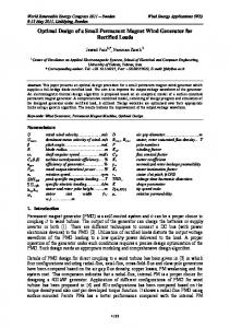
The CASTEM model uses simple beam elements to model the five bar mechanism. Each link is modeled with 8 elements. The actuated coordinates are considered to be fixed and are treated as cantilevered beams. The nodes corresponding to the passive coordinates are free, and establish pinned connections for two un-actuated links. The first three modes of the actuated beams can be seen in figure 2.9.

Figure 2.9: The first three modes shapes as per CASTEM at position [0.35, 0.3]

33

Chapter 2. Modeling

2.3 Model Verification

As the modeling techniques are inherently different [6], it was found that the third natural frequency in the AMM, corresponds to the 5th or 6th mode in the FEA. This discrepancy is due to the fact that the FEA model allows the bending of the two distal links, whereas the AMM assigns a traction-compression modal series to these two links. This property is both the advantage and disadvantage of the assumed modes method. Unless the structure is well understood, important structural behaviours may be overlooked. Nevertheless, it can be seen that the results are satisfactory, with the first and second natural frequencies being accurate within, at worst, a 3.126% accuracy. As expected, the third natural frequency shows some deviation, with an error of up to 8.563% at the [0.2, 0.5] end effector position.

Effector Position [X, Y ]

1st Natural Frequency [Hz] AMM

FEA

2nd Natural Frequency [Hz] %Error

AMM

FEA

3rd Natural Frequency [Hz] %Error

AMM

FEA

%Error

15

[0.5, 0.1] [0.4, 0.2] [0.35, 0.3] [0.3, 0.4] [0.2, 0.5] [0.0, 0.6]

116.61 136.13 134.85 127.86 124.2 140.64

115.32 134.59 133.42 126.42 122.51 136.41

1.119 1.144 1.072 1.139 1.379 3.101

210.68 157.27 156.07 168.02 183.25 226.67

206.51 156.19 153.03 166.93 182.06 219.80

2.019 0.691 1.987 0.653 0.654 3.126

1877.3 1921.1 1923.2 1917.2 1908.1 1775.4

1879.5 1833.4 1833.7 1806.2 1757.6 1890.2

0.117 4.783 4.881 6.145 8.563 6.073

Table 2.3: Natural Frequencies at Various Robot Configurations

In the case of a planar five bar mechanism, the links are pin connected and the bending modes are not excited as they are only exposed to tensile and compressive forces, giving support to the approach taken in the AMM. To incorporate this assumption in the FEA, the second moment of inertia of the distal links were increased by a factor of 5. This increase in inertia, effectively allows the third natural frequency of the FEA to coincide with the AMM (table 2.4), and drastically reduces the percentage error.

Effector Position [X, Y ] [0.5, 0.1] [0.4, 0.2] [0.35, 0.3] [0.3, 0.4] [0.2, 0.5] [0.0, 0.6]

3rd Natural Frequency [Hz] AMM 1877.3 1921.1 1923.2 1917.2 1908.1 1775.4

FEA 1874.3 1916.8 1917.9 1914.9 1906.1 1710.3

%Error 0.160 0.224 0.276 0.120 0.105 3.806

Table 2.4: Third natural frequency with adjusted inertia in the FEA

34

Chapter 2. Modeling

2.3 Model Verification

In their study on the vibrational performance of parallel robots, Piras et al [21], perform a frequency analysis of a region in the workspace of a 3-PRR robot, a similar study is performed here, the frequency distribution for the first three natural frequencies are shown in figures 2.10, 2.11 and 2.12. The workspace boundaries correspond to the type I (serial singularities) present in this robotic structure. The relative sizing of the links do not allow a type II (parallel singularity) to be obtained in the workspace. First natural frequency distribution 0.6

14 30

70

70

0.5 70

0 14

13

70

14 0

130

70

00 14 7

0

−0.1

0 13

70

70

70

130

0

14

0

130

0.1

140 1 0 140670

0 16 130

0

0 14

140

0.2

130

13

0.3

70

130

140

y [m]

0.4

130

130

70

−0.2 −0.5

0 x [m]

0.5

Figure 2.10: Contour plot of first natural frequency in workspace

Second natural frequency distribution 0.6 17

170

40 01510

170 150

0.5

0

117500 140

170

70500 1141

150 140

170 140 170

1

0

17

y [m]

0 140 15

0

15

70

1141750 00

−0.1

170

0

17

0

150

17 0 0

15 150170 140

0.1

140

17

1

0.3 0.2

0 17 0 15

50

140

0.4

151400

117500 1145 140 170 00

117 140500

−0.2 −0.5

0 x [m]

0.5

Figure 2.11: Contour plot of second natural frequency in workspace

35

Chapter 2. Modeling

2.3 Model Verification

Third natural frequency distribution 400 1000 1901

0.6

40 0 10 00 19 01

0.5 0

10 00 19 01

30

1901

193

0

190

4001000

1

40 0 1000

1

190

0

1930 1

19 1000 0

400

01000

40

400

40

00

10

1930

1930

0

1901

0.1

19

19

19 30

0.3

193

0

30

00

y [m]

0.4

0.2

1930

40010

40

1901 400 1000

−0.1 −0.2 −0.5

0 x [m]

0.5

Figure 2.12: Contour plot of third natural frequency in workspace

From the figures two key characteristics may be observed: • Natural frequencies in the "centre" workspace tend to be low • The natural frequency drops dramatically as one approaches the singularity conditions

36

Chapter 2. Modeling

2.3 Model Verification

Tool Mass Effects The previous studies did not incorporate the mass of the effector tool or payload. This mass greatly affects the structural resonances of the robot by altering the natural frequencies. This is to say that the structural resonance of the robot is a function of its configuration and its loading condition. The effect of the tool mass mtool , is investigated for the following cases: 0kg, 1kg, 10kg and 100kg, see figure 2.13:

mtool = 1kg

mtool = 0kg 0.6

0 0.5

−0.5

0 x [m]

y [m]

mtool = 10kg 0.6

15

0

40 0 x [m]

0.2

15

y [m]

50

40

y [m]

0.4

0.5

15

−0.5

20 15

10

−0.5

10

60 50

0.2 0

0.6

1015

0.4

0.5

mtool = 100kg

40

40

100 110 120 100 110

0

0 x [m]

0.2

10

130

−0.5

140

0

160 130

140

130

0.2

0.4

130

y [m]

0 13

0.4

100

100 1 00

0.6

10 0 x [m]

0.5

Figure 2.13: First natural frequency in workspace as a function of tool mass

It can be seen that increasing the mass of the tool decreases the resonance frequencies. The major frequencies in the workspace are 130Hz, 100Hz, 40Hz and 15Hz respectively. The effect of payload on the robot would be similar, it may at this point be anticipated that the control strategies for the robot should be adapted to instances with and without payload.

37

Chapter 2. Modeling

2.3.3

2.3 Model Verification

Deformation Analysis

To verify the accuracy of the stiffness matrix, the deformation of the robotic structure is investigated under certain loading conditions. The end effector is placed at the positions shown in figure 2.14. A comparison between the deformations predicted in the AMM and the FEA are presented in tables 2.5 and 2.6. Deformations − Fy = 100N ← dy : 0.0082982mm

0.6

atX= [0, 0.6]0

← dy : 0.058585mm

0.5

atX= [0.2, 0.5]0

← dy : 0.082869mm

0.4

atX= [0.3, 0.4]0

← dy : 0.085743mm

y [m]

0.3

atX= [0.35, 0.3]0

← dy : 0.090899mm

0.2

atX= [0.4, 0.2]0

← dy : 0.16579mm

0.1

atX= [0.5, 0.1]0

0 −0.1 −0.2 0

0.2

0.4 x [m]

0.6

0.8

Figure 2.14: Configurations for deformation verification

Static deformations on the structure may be calculated from evaluating the static equilibrium of the robot. As the robot is assumed to be at rest, q˙ and q ¨ are taken as 0:      I 0 CTna ×np 0na ×1 τa 0 I BTn ×n  τe  +  0ne ×1  = 0 (2.105) e p Floadnp ×1 λ 0 0 ATnp ×np Gravitational effects owing to the mass of the links and the tool are ignored and the observed deformations are only due to the applied load. Solving for λ: λ = −AT

−1

Fload

(2.106)

Solving for τe : τe + BT λ = 0

τe = BT AT

−1

(2.107)

Fload = −Je Fload

Based on Hooks Law, the following applies τe = Kqe , therefore: qe = K−1 τe

(2.108)

The results in tables 2.5 and 2.6 show very good accuracy. Poorer accuracy is however observed at positions [0.5, 0.1] and [0.0, 0.6]. These two configurations are closer to the singular positions, giving rise to poorer conditioning of the Jacobian matrices. It is notable that the structure becomes less stiff at these positions.

38

Chapter 2. Modeling

2.3 Model Verification

Fx = 100N

Effector Position

[X, Y ] [0.5, 0.1] [0.4, 0.2] [0.35, 0.3] [0.3, 0.4] [0.2, 0.5] [0.0, 0.6]

x − y AMM [µm] 15.082 68.452 75.714 79.073 95.935 73.49

-14.053 -21.306 -21.099 -34.036 -39.097 0.00277

x − y FEA [µm] 15.441 68.6531 75.935 79.374 96.3735 75.236

-14.366 -21.362 -21.130 -34.061 -39.112 7E-12

%Error 2.323 0.293 0.291 0.379 0.455 2.321

Table 2.5: Deformation under Fx = 100N

Fy = 100N

Effector Position

[X, Y ] [0.5, 0.1] [0.4, 0.2] [0.35, 0.3] [0.3, 0.4] [0.2, 0.5] [0.0, 0.6]

x − y AMM [µm] -14.077 -21.283 -21.077 -34.028 -39.1 0.00039

165.79 90.899 85.745 82.869 58.585 8.2982

x − y FEA [µm] -14.366 -21.362 -21.130 -34.061 -39.112 0.0653

166.347 91.15 85.924 83.012 58.736 8.4985

%Error 0.347 0.280 0.211 0.161 0.187 2.360

Table 2.6: Deformation under Fy = 100N In the next chapter various pick and place trajectories are developed and discussed. The trajectories are compared and contrasted, and the frequency content is presented.

39

Chapter 3

Trajectory Design Pick-and-place tasks are commonly performed by industrial robots responsible for packing and assembly operations [8, 10]. The procedure transfers an object from one workplace to another [10]. The scope of this report is limited to the study of pick-and-place paths followed in a two dimensional, planar space. The movement shown in figure 3.1 may nominally be achieved with a 2DOF robot. This standardized geometric path is referred to as the Adept cycle and has dimensions of h = 25mm and l = 350mm [13].

Figure 3.1: Pick-and-place trajectory.

The standard adept cycle, shown in 3.1 has square corners, and introduce discontinuity in acceleration when traversed. To overcome these discontinuities extremely high torques must be generated at the actuators, this, coupled with the inertial effect of the moving system, give rise to unwanted vibrations. To avoid these discontinuities the adept cycle is made smooth by introducing blends at the corners [8]. The rate at which the geometric path is followed is also a source of vibration. The motion profile, governing the traversal of the path, must be well chosen and designed to minimize excitation of resonances in the structure. The sampling of the geometric path as determined by the motion profile gives rise to the trajectory. This chapter first introduces some geometric paths, followed by the presentation of typical motion profiles. Finally, the resultant trajectories will be compared and discussed.

Chapter 3. Trajectory Design

3.1

3.1 Geometric Path

Geometric Path

In this section various geometric curves will be introduced for blending purposes. The following curves will be seen: • Clothoid Curves • Lamé Curves • Polar Polynomials Gauthier et al.[8] propose the blending dimensions shown in figure 3.2 to optimize the energy consumed by a SCARA robot performing pick and place tasks. In the image, d corresponds to the vertical blending length, and e to the horizontal blending length of a corner.

Figure 3.2: Adept half cycle using a Lamé curve [8]

3.1.1

Clothoids

Clothoids curves are discussed in great detail in path planning for autonomous vehicle literature. These curves are the time optimal solution for given constraints in jerk[14]. Clothoid curves are defined within the Cartesian frame as follows: x(θ) = aC(θ)

y(θ) = aS(θ)

(3.1)

Where a is the clothoid sharpness and C(θ) and S(θ) are the Fresnel Integrals: 1 C(θ) = √ 2π

Z 0

θ

cos u √ du u

1 S(θ) = √ 2π

Z 0

θ

sin u √ du u

(3.2)

A clothoid curve is characterized by the curvature function [27]: √ 2πθ dθ(s) = κ(θ) = ds a Kanayama and Miyake, [14] show that the Cartesian coordinates of a curve may be derived from its curvature function as follows: h i Rs Rt x(s) = 0 cos θ0 + 0 κ(θ)dθ dt i h Rt Rs y(s) = 0 sin θ0 + 0 κ(θ)dθ dt (3.3) Skeleton ray diagrams are used to constrain the blending of two consecutive straight line segments. Clothoids are used in pairs and may be used to perform symmetric or un-symmetric blending. Each cloithoid segment, i, is integrated from 0 to θi to find the resultant curve in Cartesian coordinates.

41

Chapter 3. Trajectory Design

3.1 Geometric Path

Symmetric Blending In symmetric blending the rays forming the skeleton diagram have equal lengths and the generated blend consists of two clothoids with equal sharpness, a. The relative angle between the two rays α is known as well as the length of each ray d. The two clothoids meet at P. From inspection one can see that the blending occurs between 0 and α2 (figure 3.3).

Figure 3.3: Symmetric blending ray diagram [27] The relative angle α and the length of each ray are related by: α α α aC + aS tan = d 2 2 2 | {z } | {z } x

y

The clothoid sharpness, a, can thus be found: a=

C

α 2




d +S

α 2




tan α2

(3.4)

Un-symmetric Blending In un-symmetric blending, the ray lengths d and e are not equal (see figure 3.4). The blending curve is generated by two clothoids A0 and A1 with associated parameters a0 , θ0 and a1 and θ1 respectively. As clothoid curvature is linear with respect to the inverse sharpness a1 , certain restrictions to blending apply [27]. Defining, k=

First Condition:

d >1 e k+cos α sin α


21 ( 4 for η ≤ 21 tf 2 s¨(η) = (3.28) − tf42 for η > 21

Motion Profile in Position 1 0.8 s

0.6 seventh bangbang trapezoidal 1/4 trapezoidal 1/8

0.4 0.2 0

0

0.2

0.4

0.6

η

Motion Profile in Velocity

0.8

1

Motion Profile in Acceleration

2 5 sdd

sd

1.5 1 0.5 0

0 −5

0

0.5 η

1

0

0.5 η

Figure 3.7: Motion profiles generated for tf = 1

48

1

Chapter 3. Trajectory Design

3.3

3.3 Trajectory Characteristics

Trajectory Characteristics

In this section, the effect of transversing a particular geometric path with a given motion profile is studied. Essentially, the motion profile dictates the rate at which the Cartesian coordinates are sampled from the geometric path.

Motion Profiles 7th order polynomial Bang-bang 1 4 Trapezoidal 1 8 Trapezoidal

Geometric Paths Lamé curve Clothoid pair Polar polynomial

Table 3.3: Tested motion profiles and geometric paths

The profiles and paths listed in table 3.3 allow 12 different path-profile combinations to be analyzed. At this point, the motion profiles are generated for a cycle time of 1 second, various characteristics of the generated trajectories may then be investigated. The 14 and 18 trapezoidal profiles refer to acceleration t t durations of 4f and 8f respectively2 . As the cycle time is fixed at tf = 1, it can be seen, as in figure 3.7 that the trapezoidal trajectories require higher accelerations than the bang-bang trajectories.

Task Space Table 3.4 shows a comparison of the velocity and acceleration characteristics of each trajectory. In the table red indicates the highest value in either velocity or acceleration performance, while blue indicates the lowest value. A trend that can be observed is that the Lamé curve requires higher velocities and accelerations, due to the fact the it has the longest curve length (table 3.1).

Motion Profiles order polynomial Bang-bang 1 4 Trapezoidal 1 8 Trapezoidal

7th

Velocity [m/s] Lamé Clothoid Polar 0.84068 0.83347 0.83608 0.76753 0.76095 0.76333 0.51242 0.50802 0.50962 0.43921 0.43545 0.43681

Acceleration [m/s2 ] Lamé Clothoid Polar 7.7818 7.3686 7.0384 5.1687 4.7268 4.4662 6.8895 6.2916 5.9544 11.8115 10.7638 10.0453

Table 3.4: Task space velocity and acceleration comparison of generated trajectories

2

Where tf is the cycle time

49

Chapter 3. Trajectory Design

3.3 Trajectory Characteristics

The generated trajectories are presented in figures 3.8, 3.9 and 3.10. Lamé Curve − End Effector Velocity Lamé Curve − End Effector Acceleration

seventh bangbang trapezoidal 1/4 trapezoidal 1/8

0.3

seventh bangbang trapezoidal 1/4 trapezoidal 1/8

8

0.2 6

ydd [m/s2]

yd [m/s]

0.1

0

4 2

−0.1

0

−0.2

−2

−0.3

−4 −8 0

0.1

0.2

0.3

0.4 xd [m/s]

0.5

0.6

0.7

−6

−4

−2

0

2

4

6

8

xdd [m/s2]

0.8

Figure 3.8: Lamé curve trajectories Clothoid Pair − End Effector Velocity Clothoid Pair − End Effector Acceleration

seventh bangbang trapezoidal 1/4 trapezoidal 1/8

0.3

seventh bangbang trapezoidal 1/4 trapezoidal 1/8

8

0.2 6

ydd [m/s2]

yd [m/s]

0.1

0

4 2

−0.1

0

−0.2

−2

−0.3

−4 −8 0

0.1

0.2

0.3

0.4 xd [m/s]

0.5

0.6

0.7

−6

−4

−2

0

2

4

6

8

xdd [m/s2]

0.8

Figure 3.9: Clothoid pair trajectories Polar Polynomial− End Effector Velocity

0.2

6

0.1

4

0

2

−0.1

0

−0.2

−2

−0.3

seventh bangbang trapezoidal 1/4 trapezoidal 1/8

8

ydd [m/s2]

yd [m/s]

Polar Polynomial − End Effector Acceleration

seventh bangbang trapezoidal 1/4 trapezoidal 1/8

0.3

−4 −8 0

0.1

0.2

0.3

0.4 xd [m/s]

0.5

0.6

0.7

−6

−4

−2

0 xdd [m/s2]

0.8

Figure 3.10: Polar polynomial trajectories

50

2

4

6

8

Chapter 3. Trajectory Design

3.3 Trajectory Characteristics

Joint Space The next study investigates the effect of trajectory following on the five bar mechanism. The inverse geometric and kinematic models for the rigid case (sections 2.2.1 and 2.2.3) are used to compute the actuated joint trajectories. The generated joint trajectories are assessed with respect to: • motion profile - geometric path combinations • cycle times • blending lengths Figures 3.11, 3.12 and 3.13 show the trajectories in the joint space for tf = 1. The spectral content of each signal in acceleration is determined. Each figure shows the Power Spectral Density function of each signal, relating distribution of energy in the signal to frequency. This distribution of energy is important as it gives an indication to the extent whereby the resonance frequencies of the structure will be excited by each trajectory. It can be observed that the spectral content of the 7th degree polynomial is much more forgiving than those of the trapezoidal and bang-bang profiles.

Joint Trajectory in Position

Joint Trajectory in Velocity 1

seventh bangbang trapezoidal 1/4 trapezoidal 1/8

3.2

0 qd11 [rad/s]

3 q11 [rad]

Lamé Curve

2.8 2.6 2.4 2.2

−1

−2 seventh bangbang trapezoidal 1/4 trapezoidal 1/8

−3

2 0

0.2

0.4

0.6 t [s]

0.8

1

0

0.2

0.4

Joint Trajectory in Acceleration

0.6 t [s]

0.8

Power Spectrum

30

seventh bangbang trapezoidal 1/4 trapezoidal 1/8

20 10

2

10

0 PSD

qdd11 [rad/s2]

1

−10 −20

0

10 seventh bangbang trapezoidal 1/4 trapezoidal 1/8

−30 −40 −50 0

0.2

0.4

0.6 t [s]

0.8

−2

10

1

0

100

200

300 400 Frequency [Hz]

500

600

700

Figure 3.11: Lame curve joint space trajectory and spectral content

The characteristic features of each plot are shown in table 3.5:

Motion Profiles order polynomial Bang-bang 1 4 Trapezoidal 1 8 Trapezoidal

7th

Velocity [rad/s] Lamé Clothoid Polar 0.84045 0.8157 0.75216 0.75156 0.73162 0.68131 0.86783 0.8448 0.78669 1.1363 1.1061 1.0300

Acceleration [rad/s2 ] Lamé Clothoid Polar 25.0858 25.3279 21.2023 16.4343 16.4834 13.7179 21.8879 21.9759 18.1215 37.432 37.6681 30.9457

Table 3.5: Characteristic features of joint space trajectories

51

Chapter 3. Trajectory Design

3.3 Trajectory Characteristics

Clothoid Pair

Joint Trajectory in Position

0 qd11 [rad/s]

q11 [rad]

3 2.8 2.6

Joint Trajectory in Velocity

1

seventh bangbang trapezoidal 1/4 trapezoidal 1/8

3.2

2.4 2.2

−1

−2 seventh bangbang trapezoidal 1/4 trapezoidal 1/8

−3

2 0

0.2

0.4

0.6 t [s]

0.8

1

0

0.2

0.4

Joint Trajectory in Acceleration

0.6 t [s]

0.8

Power Spectrum 4

10

30

seventh bangbang trapezoidal 1/4 trapezoidal 1/8

20 10

2

10

0 PSD

qdd11 [rad/s2]

1

−10

0

−20

10

seventh bangbang trapezoidal 1/4 trapezoidal 1/8

−30 −40 −50 0

0.2

0.4

0.6 t [s]

0.8

−2

10

1

0

100

200

300 400 Frequency [Hz]

500

600

700

Figure 3.12: Clothoid pair joint space trajectory and spectral content

Joint Trajectory in Position

Polar Polynomial

Joint Trajectory in Velocity

1 seventh bangbang trapezoidal 1/4 trapezoidal 1/8

3.2

0 qd11 [rad/s]

q11 [rad]

3 2.8 2.6 2.4 2.2

−1

−2

seventh bangbang trapezoidal 1/4 trapezoidal 1/8

−3

2 0

0.2

0.4

0.6 t [s]

0.8

1

0

0.2

0.4

Joint Trajectory in Acceleration

0.6 t [s]

0.8

1

Power Spectrum

30 seventh bangbang trapezoidal 1/4 trapezoidal 1/8

20 2

10 0 PSD

qdd11 [rad/s2]

10

−10 −20

0

10 seventh bangbang trapezoidal 1/4 trapezoidal 1/8

−30 −40 −50 0

0.2

0.4

0.6 t [s]

0.8

−2

10

1

0

100

200

300 400 Frequency [Hz]

500

600

700

Figure 3.13: Polar polynomial joint space trajectory and spectral content

The general trend of the motion profile-trajectory combination can be observed in figure 3.14. While the difference is not great, it can be seen that Lamé curves correspond to trajectories with lower energy while polar polynomials correspond to higher energies.

52

Chapter 3. Trajectory Design

3.3 Trajectory Characteristics

Power Spectrum seventh−lame seventh−clothoid seventh−polar

4

10

3

10

2

PSD

10

1

10

0

10

−1

10

−2

10

0

100

200

300 400 Frequency [Hz]

500

600

700

Figure 3.14: Spectral content for the various geometric paths based on a 7t h order polynomial traversal Figures 3.15 and 3.16 show the effect of varying the cycle time and the blending length d3 . As expected, decreasing the cycle time tf inflates the energy content at all frequencies. Furthermore, the shorter the blending length, and thus, the sharper the corner, the higher the energy content of the input signal.

Seventh−Lamé Trajectories

Joint Trajectory in Position

seventh tf = 1

3.2

seventh tf = 0.5

0

seventh tf = 0.25

−2 qd11 [rad/s]

q11 [rad]

3

Joint Trajectory in Velocity

2

2.8 2.6 2.4

−4 −6 −8

seventh tf = 1

−10 2.2

−12

2

−14 0

0.2

0.4

0.6

0.8

1

seventh tf = 0.5 seventh tf = 0.25 0

0.2

0.4

0.6

t [s]

t [s]

Joint Trajectory in Acceleration

Power Spectrum

0.8

1

400 seventh tf = 1 10

0 PSD

qdd11 [rad/s2]

seventh tf = 0.5

4

200

seventh tf = 0.25

2

10

−200 0

10

seventh tf = 1

−400

seventh tf = 0.5 seventh tf = 0.25

−600 0

0.2

0.4

0.6

0.8

−2

10 1

0

t [s]

100

200

300 400 Frequency [Hz]

500

600

700

Figure 3.15: Spectral content for seventh-lamé trajectories for cycle times of tf = 1, tf = 0.5 and tf = 0.25

3

the symmetric case is considered, i.e. d = e

53

Chapter 3. Trajectory Design

3.3 Trajectory Characteristics

Effect of blending length

Joint Trajectory in Position

0 qd11 [rad/s]

q11 [rad]

3

Joint Trajectory in Velocity

1

seventh d = 25mm seventh d = 12.5mm seventh d = 6.125mm

3.2

2.8 2.6 2.4 2.2

−1

−2 seventh d = 25mm seventh d = 12.5mm seventh d = 6.125mm

−3

2 0

0.2

0.4

0.6

0.8

1

0

0.2

0.4

t [s]

0.6

0.8

1

t [s]

Joint Trajectory in Acceleration

Power Spectrum 4

seventh d = 25mm seventh d = 12.5mm seventh d = 6.125mm

10

50

2

10 −50

PSD

qdd11 [rad/s2]

0

0

−100

10 seventh d = 25mm seventh d = 12.5mm seventh d = 6.125mm

−150

0

0.2

0.4

0.6

0.8

−2

10 1

0

t [s]

100

200

300 400 Frequency [Hz]

500

600

700

Figure 3.16: Spectral content for seventh-lamé trajectories for symmetric blending lengths of d = 25mm, d = 12.5mm and d = 6.125mm

Trajectory Discussion From the analysis done in section 3.3, it is clear that there is a trade-off between the cycle time and the amount of energy distribution in the trajectory signals. The following conclusions may be drawn: • Shorter curve lengths require lower accelerations • Lower cycle times require higher accelerations and increase the spectral content of the signal at all frequencies • Sharper corners increase the spectral content of the signal at all frequencies In the next section the elastodynamic model of the five bar mechanism will be excited with the trajectories discussed in this section.

54

Chapter 4

Simulation Adept Technology, Inc. [13], manufacturers of the worlds fastest robot, specify the following cycletime payload combinations for the standard adept cycle:

Adept Cycle (Std.) - Sustained Standard Cycle: 25/305/25 (mm) Payload [kg] Cycle time tf [s] 0.1 0.30 1.0 0.36 2.0 0.37 4.0 0.41 6.0 0.43 Table 4.1: Adept cycle times and payloads

Trajectory in Workspace 0.6 Workspace Trajectory

0.5 0.4

y[m]

0.3 0.2 0.1 0 −0.1 −0.5

0 x[m]

0.5

Figure 4.1: Position of the trajectory in the workspace (gravity is taken upwards)

In this section, it is assumed that a perfect controller is available. The inverse dynamic model (section 2.1.9) is used to evaluate the vibratory performance of the five bar mechanism as it traverses the various trajectories (see figure 4.1). The simulations are conducted for the 0.1kg and 6.0kg cases listed in table 4.1. The simulation is run at a sampling frequency of 10M Hz. The following results will be presented and discussed:

Chapter 4. Simulation

4.1 Simulation Set 1

• Trajectory following in the task space • Required joint torques • Excited vibrations • Spectral content of the vibratory signal

4.1 4.1.1

Simulation Set 1: 0.1kg tf = 0.3s Vibrational Domain

The frequency analysis developed in section 2.3.2, may be used to determine the evolution of the system’s natural frequency as it follows the adept cycle. Figure 4.2 represents the frequencies present on a cycle with clothoid blending. It can be seen that the first natural frequency varies with ±2Hz about 126Hz, while the margin increases to ±7.5Hz about 1912Hz for the third natural frequency.

Frequency [Hz]

First Natural Frequency 128 126

0

0.2

0.4

0.6

0.8

1

0.8

1

0.8

1

Frequency [Hz]

s [m]

Second Natural Frequency 170 160 0

0.2

0.4

0.6 s [m]

Frequency [Hz]

Third Natural Frequency 1918 1914 1910 1906 0

0.2

0.4

0.6 s [m]

Figure 4.2: Frequency distribution along Adept Cycle with a 100g payload. Line styles: - Lamé, - Clothoid, ... Polar

4.1.2

Simulation Results

The simulation results are now presented. In each figure, 12 results are superposed, line colour represents the different motion profiles used. Figure 4.3 shows the velocity and accelerations obtained in the task space with the inclusion of elastic deformation.

Task Space The effect of deformation is most notable in the acceleration plot. The emergent trajectory does not follow the expected trajectory in acceleration. At the end of the cycle time tf , the relative position between the actual and expected position, the velocity and the acceleration of the end effector as averaged per motion profile is given in table 4.2. Ideally, the relative position between the actual and desired end effector positions is 0, while the desired velocity and acceleration are 0 in both cases. From the table it can be observed that the end effector states in position are the best for the bangbang profile, this due to the fact that the bang-bang profile has the lowest acceleration value. What is interesting to note, is that the 7th degree polynomial offers the best performance in velocity and acceleration error, owing to the continuity and smoothness of its acceleration profile at this point.

56

Chapter 4. Simulation

4.1 Simulation Set 1

End Effector Velocity seventh bangbang trapezoidal 1/4 trapezoidal 1/8

1

End Effector Acceleration 120 100 80

0.5

ydd [m/s2]

yd [m/s]

60

0

40 20 0 −20

−0.5 −40 −60 −1

−150

−100

−50

0

50

100

150

xdd [m/s2] 0

0.5

1

1.5 xd [m/s]

2

2.5

Figure 4.3: Simulation results for a 100g payload in the task space

Motion Profiles 7th order polynomial Bang-bang 1 4 Trapezoidal 1 8 Trapezoidal

Position [mm] xrel yrel -0.00349 -0.01559 0.00068 0.00746 0.00184 0.01573 0.00671 0.04156

Velocity x˙ 0.00074 0.00042 -0.00065 -0.00559

[m/s] y˙ 0.00081 0.00589 0.00647 0.00698

Acceleration [m/s2 ] x ¨ y¨ 0.4998 0.3127 0.3998 -16.626 0.6456 -22.756 0.37523 -41.73167

Table 4.2: Terminal end-effector state at tf = 0.3 for a payload of 100g

Motion Profiles order polynomial Bang-bang 1 4 Trapezoidal 1 8 Trapezoidal

7th

Velocity [m/s] Lamé Clothoid Polar 2.8032 2.8010 2.7881 2.5689 2.5668 2.5549 1.7259 1.726 1.714 1.5130 1.5028 1.5123

Acceleration [m/s2 ] Lamé Clothoid Polar 88.652 90.736 89.602 59.677 61.849 53.019 79.671 83.456 71.594 154.65 146.94 128.40

Table 4.3: Maximum task space velocity and acceleration for a payload of 100g and a cycle time of tf = 0.3s

Joint Torques The resultant joint torques show the effect of the vibrations on the required torque. The oscillations in the torque signal are more pronounced for signals with discontinuities in vibration. From the behaviour of the signals, it is clear to see that the vibrations are excited at these discontinuities. The bang-bang t profile shows excitation at the cycle mid-point while the trapezoidal signals show excitation at 4f and tf 8 . The maximum torques required for each signal are summarized in table 4.4.

57

Chapter 4. Simulation

4.1 Simulation Set 1

Joint Torques: Tau11 30 20

Tau [N/m]

10 0 −10 −20

seventh bangbang trapezoidal 1/4 trapezoidal 1/8

−30 −40 −50 0

0.05

0.1

0.15 t [s]

0.2

0.25

0.3

Joint Torques: Tau21 50 40

Tau [N/m]

30 20 10 0

seventh bangbang trapezoidal 1/4 trapezoidal 1/8

−10 −20 −30 0

0.05

0.1

0.15 t [s]

0.2

0.25

0.3

Figure 4.4: Joint torques for a 100g payload. Line styles: - Lamé, - - Clothoid, ... Polar

Vibrations The elastic coordinates qe are also obtained through the solution of the inverse dynamic model. The elastic coordinates in bending and in tension-compression are presented in figures 4.5 and 4.6 respectively.

qe11 and qe21

−5

x 10

qe [m]

5

0 seventh bangbang trapezoidal 1/4 trapezoidal 1/8

−5 0

0.05

0.1

0.15 t [s]

0.2

0.25

0.3

qed11 and qed21

qed [m/s]

0.01 0

0.25

seventh bangbang trapezoidal 1/4 trapezoidal 1/8 0.3

0.25

seventh bangbang trapezoidal 1/4 trapezoidal 1/8 0.3

−0.01 −0.02 0

0.05

0.1

0.15 t [s]

0.2

qedd11 and qedd21 15 qedd [m/s2]

10 5 0 −5 −10 0

0.05

0.1

0.15 t [s]

0.2

Figure 4.5: Elastic Coordinates in Bending for a 100g payload. Line styles: - Lamé, - - Clothoid, ... Polar

58

Chapter 4. Simulation

4.1 Simulation Set 1

qe12 and qe22

−7

x 10 4

qe [m]

2 0 −2

0.25

seventh bangbang trapezoidal 1/4 trapezoidal 1/8 0.3

0.25

seventh bangbang trapezoidal 1/4 trapezoidal 1/8 0.3

−4 −6 0

0.05

0.1

0.15 t [s]

0.2

qed12 and qed22

−4

x 10

qed [m/s]

1 0 −1 −2

0

0.05

0.1

0.15 t [s]

0.2

qedd12 and qedd22 0.15 qedd [m/s2]

0.1 0.05 seventh bangbang trapezoidal 1/4 trapezoidal 1/8

0 −0.05 −0.1 0

0.05

0.1

0.15 t [s]

0.2

0.25

0.3

Figure 4.6: Elastic Coordinates in Tension-Compression for a 100g payload. Line styles: - Lamé, - Clothoid, ... Polar

The spectral content of the signals may be analyzed to identify the excited frequencies. The signal is shown between 0 and 700Hz as there is very little activity at higher frequencies. The results show that the frequencies coinciding with the first and second resonances are excited. This is to be expected, referring to figure 3.15, it can be seen that the energy of the input signal attenuates greatly after a frequency of 300Hz. Power Spectrum Bending 8000 6000 PSD

seventh bangbang trapezoidal 1/4 trapezoidal 1/8

X: 125.8 Y: 8286 X: 161.3 Y: 6677

4000 2000

0

100

200

300 400 Frequency [Hz]

500

600

700

Power Spectrum Tension−Compression 80 60 PSD

seventh bangbang trapezoidal 1/4 trapezoidal 1/8

X: 125.8 Y: 85.1 X: 161.3 Y: 63.32

40 20 0

100

200

300 400 Frequency [Hz]

500

600

700

Figure 4.7: Spectral Distribution for a 100g payload. Line styles: - Lamé, - - Clothoid, ... Polar

59

Chapter 4. Simulation

4.1 Simulation Set 1

The results of this simulation set is summarized in table 4.4. The table firstly shows the maximum torque required. Secondly the root mean square (RMS) value of the acceleration error is computed using equation 4.1. Lastly, the maximum deflection in the elastic coordinates is noted, this maximum deflection occurs in the links in bending. s
2 Pn ¨ ¨ 1 Xdesired − Xactual RM Serror = (4.1) n where n is the number of data points

Lamé

Motion Profiles 7th order polynomial Bang-bang 1 4 Trapezoidal 1 8 Trapezoidal Motion Profiles 7th order polynomial Bang-bang 1 4 Trapezoidal 1 8 Trapezoidal Motion Profiles 7th order polynomial Bang-bang 1 4 Trapezoidal 1 8 Trapezoidal

Clothoid Polar Torque [N m] 33.6384 32.737 33.0867 23.9012 23.1011 22.3707 30.6662 29.4722 28.56 51.3054 45.9056 47.4447 RMS Acceleration Error [m/s2 ] 3.3563 3.8525 6.2169 5.2095 5.3852 5.7002 5.2813 5.6053 5.9695 9.8592 8.7226 9.5968 Max Deflection [mm] 0.04339 0.04223 0.04269 0.03082 0.02979 0.02885 0.03957 0.03802 0.03684 0.0663 0.05931 0.06134

Table 4.4: Task space velocity and acceleration comparison of generated trajectories

From the table it can be seen that the worst performance, on all counts, is associated with the 18 trapezoidal profile as it requires the highest accelerations. The required torque is closely related to the path length, and thus the lowest torques correspond to the polar polynomial trajectories. The best performance in terms of the RMS acceleration error is associated with the smoothest trajectory, the 7th degree polynomial-Lamé curve.

60

Chapter 4. Simulation

4.1 Simulation Set 1

Errors in the Task Space The norm of the error in the task space is shown in figure 4.8. An understanding of the residual deformations and energies in the signal may be obtained from studying table 4.5. While the smoothness of a curve significantly decreases the residual error, the maximum acceleration achieved along a path plays a dominant role. The trends correspond to those seen in 3.14. The polar polynomial has slightly higher spectral energy at the natural frequencies of the robot and is associated with higher residual errors. What is clear is that the smooth 7t h order curve presents the best results in the error norms. At this slower cycle speed of tf = 0.3 and low payload of 100g, the smoothness of the trajectory is the dominant factor for the level of residual activity in position. Position Error Norm seventh bangbang trapezoidal 1/4 trapezoidal 1/8

Error [mm]

0.2

0.15

0.1

0.05

0

0.05

0.1

0.15 t [s] − lame −− clothoid ...polar

0.2

0.25

Velocity Error Norm seventh bangbang trapezoidal 1/4 trapezoidal 1/8

0.06

Error [m/s]

0.05 0.04 0.03 0.02 0.01 0

0.05

0.1

0.15 t [s] − lame −− clothoid ...polar

0.2

0.25

Acceleration Error Norm 40

seventh bangbang trapezoidal 1/4 trapezoidal 1/8

35

Error [m/s2]

30 25 20 15 10 5 0

0.05

0.1

0.15 t [s] − lame −− clothoid ...polar

0.2

0.25

Figure 4.8: Error norm in the task space with a 100g payload. Line styles: - Lamé, - - Clothoid, ... Polar

61

Chapter 4. Simulation

4.2 Simulation Set 2

Lamé

Motion Profiles order polynomial Bang-bang 1 4 Trapezoidal 1 8 Trapezoidal Motion Profiles 7th order polynomial Bang-bang 1 4 Trapezoidal 1 8 Trapezoidal Motion Profiles 7th order polynomial Bang-bang 1 4 Trapezoidal 1 8 Trapezoidal 7th

Clothoid Polar Position [mm] 0.0157 0.0009 0.3109 0.0078 0.0007 0.5573 0.0160 0.0017 0.9366 0.0439 0.0049 0.2872 Velocity [m/s] 0.0009 0.0053 0.4973 0.0049 0.0050 1.0716 0.0055 0.0055 0.2611 0.0087 0.0062 0.8352 Acceleration [m/s2 ] 0.5573 0.0045 1.3193 0.4973 0.0050 1.0716 0.8352 0.0045 1.3193 1.8212 0.0083 3.0404

Table 4.5: Residual norms at end effector end points

4.2

Simulation Set 2: 6.0kg tf = 0.43s

The cycle with the heaviest payload is now investigated (table 4.1). Compared to the simulation done in the previous section (4.1), the payload is increased by a factor of 60 while the cycle time is increased by a factor of 1.43.

4.2.1

Vibrational Domain

The heavier payload transforms the frequencies present along the geometric path (compare figures 4.2 and 4.9). The first natural frequency is now located at 58Hz ± 1Hz, the second at 80Hz ± 6Hz and finally the third natural frequency at 1823Hz ± 13Hz.

Frequency [Hz]

First Natural Frequency 58.5 58 57.5 57 0

0.2

0.4

0.6

0.8

1

0.8

1

0.8

1

Frequency [Hz]

s [m]

Second Natural Frequency 85 80 75 0

0.2

0.4

0.6 s [m]

Frequency [Hz]

Third Natural Frequency 1830 1825 1820 1815 0

0.2

0.4

0.6 s [m]

Figure 4.9: Frequency distribution along Adept Cycle with a 6000g payload. Line styles: - Lamé, - Clothoid, ... Polar

62

Chapter 4. Simulation

4.2.2

4.2 Simulation Set 2

Simulation Results

Figure 4.10 shows the velocity and accelerations obtained in the task space with the inclusion of elastic deformation. With the higher payload, oscillations about the desired end position of the end effector become visible. Here the results are averaged according to the various geometric paths so that the general trends may be seen.

Task Space End Effector Velocity 0.8

End Effector Acceleration

0.6

60 50

0.4

40 30 ydd [m/s2]

yd [m/s]

0.2 0 −0.2

20 10 0 −10

−0.4

−20

seventh bangbang trapezoidal 1/4 trapezoidal 1/8

−0.6

−30 −40 −80

−60

−40

−20

0

20

40

60

80

xdd [m/s2]

−0.8 0

0.2

0.4

0.6

0.8 1 xd [m/s]

1.2

1.4

1.6

1.8

Figure 4.10: Simulation results for a 6kg payload in the task space. Line styles: - Lamé, - - Clothoid, ... Polar

Motion Profiles 7th order polynomial Bang-bang 1 4 Trapezoidal 1 8 Trapezoidal

Position [mm] xrel yrel -0.00299 -0.04231 -0.00944 -0.02703 0.01330 0.01512 -0.09179 -0.01427

Velocity [m/s] x˙ y˙ -0.00256 -0.00102 0.00801 0.00685 0.01400 0.00966 0.01707 0.02793

Acceleration [m/s2 ] x ¨ y¨ -1.1090 -2.9313 0.6245 -5.7937 -1.793 -12.188 15.75267 -11.109

Table 4.6: Averaged terminal end-effector state at tf = 0.43 for a payload of 6000g Table 4.7 shows the maximum velocities and accelerations occurring in the task space. As before, the highest accelerations are associated with the 18 trapezoidal-Lamé trajectory.

Motion Profiles order polynomial Bang-bang 1 4 Trapezoidal 1 8 Trapezoidal

7th

Velocity [m/s] Lamé Clothoid Polar 1.9581 1.9571 1.9504 1.7962 1.7943 1.787 1.2185 1.2154 1.2256 1.0761 1.074 1.076

Acceleration [m/s2 ] Lamé Clothoid Polar 48.476 47.094 50.31 32.551 31.308 31.939 47.465 46.194 45.352 82.574 82.159 74.896

Table 4.7: Maximum task space velocity and acceleration for a payload of 6kg and a cycle time of tf = 0.43

63

Chapter 4. Simulation

4.2 Simulation Set 2

Joint Torques The maximum torques required for each signal are summarized in table 4.8. Joint Torques: Tau11 100

Tau [N/m]

50

0 seventh bangbang trapezoidal 1/4 trapezoidal 1/8

−50

−100 0

0.05

0.1

0.15

0.2

0.25

0.3

0.35

0.4

t [s]

Joint Torques: Tau21 100

Tau [N/m]

50

0 seventh bangbang trapezoidal 1/4 trapezoidal 1/8

−50

0

0.05

0.1

0.15

0.2

0.25

0.3

0.35

0.4

t [s]

Figure 4.11: Joint torques for a 6000g payload. Line styles: - Lamé, - - Clothoid, ... Polar

Vibrations The elastic coordinates qe are also obtained through the solution of the inverse dynamic model. The elastic coordinates in bending and in tension-compression are presented in figures 4.12 and 4.13 respectively. Figure 4.14 shows the power spectral density of the elastic coordinates qe , the frequencies identified in section 4.2.1 are identifiable as peaks in the figure. Again, the first two modes of vibration are dominant as they are excited by the input trajectories. The results of this simulation set is summarized in table 4.8. From the table, it can be seen that high input accelerations, and thus high torques, correspond to the highest deflections (i.e. 14 trapezoidal profile), while the opposite is true for low input accelerations (i.e. bang-bang).

64

Chapter 4. Simulation

4.2 Simulation Set 2

qe

−4

11

x 10

and qe

21

qe [m]

1

0

0.35

seventh bangbang trapezoidal 1/4 trapezoidal 1/8 0.4

0.35

seventh bangbang trapezoidal 1/4 trapezoidal 1/8 0.4

0.35

seventh bangbang trapezoidal 1/4 trapezoidal 1/8 0.4

−1 0

0.05

0.1

0.15

0.2

0.25

0.3

t [s]

qed11 and qed21

qed [m/s]

0.02 0 −0.02

0

0.05

0.1

0.15

0.2

0.25

0.3

t [s]

qedd11 and qedd21

qedd [m/s2]

10 5 0 −5 −10 0

0.05

0.1

0.15

0.2

0.25

0.3

t [s]

Figure 4.12: Elastic Coordinates in Bending for with a 6kg payload. Line styles: - Lamé, - - Clothoid, ... Polar qe12 and qe22

−6

x 10 2

qe [m]

1 0

0.35

seventh bangbang trapezoidal 1/4 trapezoidal 1/8 0.4

0.35

seventh bangbang trapezoidal 1/4 trapezoidal 1/8 0.4

−1 −2 0

0.05

0.1

0.15

0.2

0.25

0.3

t [s]

qed12 and qed22

−4

x 10

qed [m/s]

4 2 0 −2 −4 0

0.05

0.1

0.15

0.2

0.25

0.3

t [s]

qedd

12

and qedd

22

qedd [m/s2]

0.2 0.1 0

seventh bangbang trapezoidal 1/4 trapezoidal 1/8

−0.1 0

0.05

0.1

0.15

0.2

0.25

0.3

0.35

0.4

t [s]

Figure 4.13: Elastic Coordinates in Tension-Compression for a 6000g payload. Line styles: - Lamé, - Clothoid, ... Polar

From the figures it can be seen that vibratory content of a given signal depends on the smoothness of the trajectory, with less oscillations attributable to the 7th degree polynomial.

65

Chapter 4. Simulation

4.2 Simulation Set 2

X: 56.82 Y: 1.092e+004

Power Spectrum Bending seventh bangbang trapezoidal 1/4 trapezoidal 1/8

10000

PSD

8000

X: 79.55 Y: 9342

6000 4000 2000 0

100

X: 56.82 Y: 171

200

300 400 Frequency [Hz]

500

PSD

700

Power Spectrum Tension−Compression seventh bangbang trapezoidal 1/4 trapezoidal 1/8

150 X: 79.55 Y: 145.4

100

600

50

0

100

200

300 400 Frequency [Hz]

500

600

700

Figure 4.14: Spectral Distribution for a 6kg payload. Line styles: - Lamé, - - Clothoid, ... Polar

Lamé

Motion Profiles order polynomial Bang-bang 1 4 Trapezoidal 1 8 Trapezoidal Motion Profiles 7th order polynomial Bang-bang 1 4 Trapezoidal 1 8 Trapezoidal Motion Profiles 7th order polynomial Bang-bang 1 4 Trapezoidal 1 8 Trapezoidal 7th

Clothoid Polar Torque [N m] 73.634 70.046 71.298 56.084 50.848 50.734 75.208 74.605 62.496 125.45 124.45 119.16 RMS Acceleration Error [m/s2 ] 2.7168 3.3724 6.641 4.5245 4.7786 5.4098 6.0193 6.3989 8.6868 10.572 10.731 13.865 Max Deflection [mm] 0.09700 0.09226 0.09392 0.07387 0.06696 0.06681 0.09911 0.09832 0.08233 0.16540 0.16408 0.13813

Table 4.8: Task space velocity and acceleration comparison of generated trajectories

The smoother the trajectory and geometric path, the less oscillatory the signal, this is revealed through the RMS error values. It can be seen that the 7th order polynomial-Lamé curve provides the best results to this regard.

66

Chapter 4. Simulation

4.2 Simulation Set 2

Errors in the Task Space The norm of the error in the task space for a payload of 6kg and a cycle time of tf = 0.43s is shown in figure 4.15. The results are slightly different to those presented in figure 4.8. Although the bang-bang profile yields a lower residual error norm in position than the 7t h order polynomial, it can be seen that the residual errors in velocity and acceleration are attenuated to greater extent by the 7th order polynomial. Position Error Norm seventh bangbang trapezoidal 1/4 trapezoidal 1/8

0.45 0.4

Error [mm]

0.35 0.3 0.25 0.2 0.15 0.1 0.05 0

0.05

0.1

0.15

0.2 t [s] − lame −− clothoid ...polar

0.25

0.3

0.35

0.4

Velocity Error Norm 0.12

seventh bangbang trapezoidal 1/4 trapezoidal 1/8

Error [m/s]

0.1 0.08 0.06 0.04 0.02

0

0.05

0.1

0.15

0.2 t [s] − lame −− clothoid ...polar

0.25

0.3

0.35

0.4

Acceleration Error Norm seventh bangbang trapezoidal 1/4 trapezoidal 1/8

35

Error [m/s2]

30 25 20 15 10 5 0

0.05

0.1

0.15

0.2 t [s] − lame −− clothoid ...polar

0.25

0.3

0.35

0.4

Figure 4.15: Error norm in the task space with a 6kg payload. Line styles: - Lamé, - - Clothoid, ... Polar

Lamé

Motion Profiles 7th order polynomial Bang-bang 1 4 Trapezoidal 1 8 Trapezoidal Motion Profiles 7th order polynomial Bang-bang 1 4 Trapezoidal 1 8 Trapezoidal Motion Profiles 7th order polynomial Bang-bang 1 4 Trapezoidal 1 8 Trapezoidal

Clothoid Polar Position [mm] 0.9355 0.0009 0.3109 4.8557 0.0007 0.5573 5.5411 0.0017 0.9366 8.7118 0.0049 0.2872 Velocity [m/s] 0.0009 0.0053 0.4973 0.0049 0.0050 1.0716 0.0055 0.0055 0.2611 0.0087 0.0062 0.8352 Acceleration [m/s2 ] 0.5573 0.0045 1.3193 0.4973 0.0087 3.8472 0.8352 0.0056 1.8212 1.8212 0.0083 3.0404

Table 4.9: Residual error norms at end effector end points for a payload of 6kg

67

Chapter 4. Simulation

4.3

4.3 Simulation Set 3

Simulation Set 3: 6.0kg tf = 0.215s

This section briefly looks the effect of halving the cycle time of the test studied in section 4.2. This study is conducted to observe the effect of the deformations in the task space to a greater extent. End Effector Position

seventh bangbang trapezoidal 1/4 trapezoidal 1/8

0.32

0.315

y [m]

0.31

0.305

0.3

0.295 0.15

0.155

0.16

0.165 x [m]

0.17

0.175

Figure 4.16: Task space position for a payload of 6kg and tf = 0.215ms Line styles: - Lamé, - - Clothoid, ... Polar

End Effector Acceleration 400

End Effector Velocity 300

seventh bangbang trapezoidal 1/4 trapezoidal 1/8

2

1.5

200

100 ydd [m/s2]

yd [m/s]

1

0.5

0

0

−100

−0.5 −200 −1 −300 −1.5 −0.5

0

0.5

1

1.5 2 xd [m/s]

2.5

3

3.5

4 −400 −400

−300

−200

−100

0

100

200

300

400

xdd [m/s2]

Figure 4.17: Task space velocity and acceleration for a payload of 6kg and tf = 0.215s Line styles: Lamé, - - Clothoid, ... Polar

In figure 4.16, it can be seen that the deformations do indeed become visible. The resultant velocities and accelerations are extremely high due to the short cycle time and the dominant inertial effects (figure 4.17).

68

Chapter 4. Simulation

4.3 Simulation Set 3

Lamé

Motion Profiles order polynomial Bang-bang 1 4 Trapezoidal 1 8 Trapezoidal Motion Profiles 7th order polynomial Bang-bang 1 4 Trapezoidal 1 8 Trapezoidal Motion Profiles 7th order polynomial Bang-bang 1 4 Trapezoidal 1 8 Trapezoidal 7th

Clothoid Polar Torque [N m] 422.36 409.52 420.02 200.69 198.11 210.11 366.02 350.89 368.43 630.69 613.85 627.44 RMS Acceleration Error [m/s2 ] 84.852 78.239 79.583 36.81 36.294 44.308 58.564 53.32 63.981 172.95 161.75 148.51 Max Deflection [mm] 0.44778 0.41406 0.41328 0.26455 0.26118 0.21627 0.35171 0.33231 0.32705 0.78559 0.73566 0.6854

Table 4.10: Comparison of results for a cycle time of tf = 0.215s Table 4.10 compares the various trajectories. As before, geometric paths sampled with the 81 trapezoidal show require the highest torques and are associated with the greatest RMS errors and deflections. The bang-bang profile requires the lowest acceleration for any given path, and shows better performance. Interestingly, it would seem that at these extreme conditions, the smoothness of the 7th degree polynomialLamé curve trajectory is not an adequate guarantee for a low RMS error.

Lamé

Motion Profiles 7th order polynomial Bang-bang 1 4 Trapezoidal 1 8 Trapezoidal Motion Profiles 7th order polynomial Bang-bang 1 4 Trapezoidal 1 8 Trapezoidal Motion Profiles 7th order polynomial Bang-bang 1 4 Trapezoidal 1 8 Trapezoidal

Clothoid Polar Position [mm] 1.1 1.6 1 0.1 0.6 0.4 0.6 1.1 0.6 2.5 1.7 2.2 Velocity [m/s] 0.057 0.0599 0.0339 0.0894 0.0883 0.1016 0.1435 0.1365 0.1104 0.4034 0.3958 0.3637 Acceleration [m/s2 ] 148.05 136.74 130.50 8.635 10.771 42.82 107.91 94.561 110.36 292.71 268.61 255.20

Table 4.11: Residual error norms at end effector end points for a payload of 6kg The error norms shown for the extremely high speed simulation in table 4.11 correspond to the findings in table 4.10. At the end of the cycle, the error norm is the best for the bang-bang profile as it invokes the lowest acceleration.

69

Chapter 4. Simulation

4.4

4.4 Simulation Set 4

Simulation Set 4: Extended Curve Lengths

This section looks at the effect of varying the blending lengths of the clothoid pairs and the Lamé curve. The blending curves with d = e = 25mm are compared with a Lamé curve with e = 125mm and a clothoid pair with e = 44mm (referred to as extended curves). The curves and the associated velocity and frequency behaviour in the task space are shown in figure 4.18.

End Effector Position 0.36

lame clothoid lameExt

0.34

clothoidExt

y [m]

0.32 0.3 0.28 0.26 −0.15

−0.1

−0.05

0 x [m]

0.05

0.1

End Effector Velocity

0.15

End Effector Acceleration

0.8

60

0.6 40

0.2

ydd [m/s2]

yd [m/s]

0.4

0 −0.2

−0.6

lame clothoid lameExt

−0.8

clothoidExt

−0.4

0

0.5

1 xd [m/s]

20 0 −20 −40 −80

1.5

−60

−40

−20

0

20

40

60

80

xdd [m/s2]

Figure 4.18: Varying blending lengths for a 6000g payload. Line styles: - Lamé, - - Clothoid, ... Polar

70

Chapter 4. Simulation

4.4 Simulation Set 4

Lamé

Motion Profiles N/A Motion Profiles 7th order polynomial Bang-bang 1 4 Trapezoidal 1 8 Trapezoidal Motion Profiles 7th order polynomial Bang-bang 1 4 Trapezoidal 1 8 Trapezoidal Motion Profiles 7th order polynomial Bang-bang 1 4 Trapezoidal 1 8 Trapezoidal

Clothoid Lamé Ext Clothoid Ext Total Path Length [mm] 0.3843 0.3840 0.3687 0.3751 Torque [N m] 73.634 70.046 29.145 46.408 56.084 50.848 34.596 36.402 75.208 74.605 39.28 44.816 125.45 124.45 70.937 70.39 RMS Acceleration Error [m/s2 ] 2.7168 3.3724 0.53046 2.3421 4.5245 4.7786 3.9246 4.0618 6.0193 6.3989 4.859 5.2756 10.572 10.731 6.5765 8.4488 Max Deflection [mm] 0.09700 0.09226 0.03833 0.06106 0.07387 0.06696 0.04556 0.04791 0.09911 0.09832 0.05173 0.05902 0.16540 0.16408 0.10245 0.09252

Table 4.12: Comparison of short and extended cycle lengths

From table 4.12, it can be observed that the shortest trajectory, the extended Lamé curve, shows the best performance on all counts. The extended Lamé curve drastically reduces the required torque, the acceleration error and the maximum deflection observed along the path. Table 4.13 shows the error norms in position, velocity and acceleration. In general it can be observed that shorter path lengths yield better results, with the 7th order polynomial providing the best results in velocity and in acceleration.

Lamé Motion Profiles N/A Motion Profiles 7th order polynomial Bang-bang 1 4 Trapezoidal 1 8 Trapezoidal Motion Profiles 7th order polynomial Bang-bang 1 4 Trapezoidal 1 8 Trapezoidal Motion Profiles 7th order polynomial Bang-bang 1 4 Trapezoidal 1 8 Trapezoidal

0.3843 0.0524 0.0219 0.0158 0.0968 0.0014 0.0085 0.0122 0.0162 1.7121 1.6179 1.6563 18.1496

Clothoid Lamé Ext Clothoid Ext Total Path Length [mm] 0.3840 0.3687 0.3751 Position [mm] 0.0503 0.0606 0.0905 0.0293 0.0125 0.0461 0.0221 0.0056 0.0320 0.0919 0.0441 0.0659 Velocity [m/s] 0.0044 0.0005 0.0058 0.0102 0.0007 0.0039 0.0130 0.0134 0.0138 0.0253 0.0081 0.0283 2 Acceleration [m/s ] 2.0211 0.3816 0.2521 2.9177 0.2230 0.8533 2.2635 1.0501 1.2532 17.4328 8.9629 12.2502

Table 4.13: Comparison of error norms on short and extended cycle lengths

This concludes the chapter on simulation. A summary is made and conclusions are drawn in the final chapter. Future work and perspectives are highlighted.

71

Chapter 5

Conclusion This master thesis investigated the use of an elastodynamic model to simulate the behaviour of a elastic five bar mechanism performing pick and place tasks. The work covered in this report can be summarized under the following categories: • Geometric and Kinematic Modeling • Elastodynamic Modeling • Trajectory Generation • Simulation

Geometric and Kinematic Modeling A rigid and elastic model of the five bar mechanism was developed. The model is simple as the number of DOF of the task and of each leg are the same. This section developed the kinematic relations relating the dependent coordinates qd to the independent coordinates qi . The elastic model introduces the elastic coordinates qe and increases the complexity. The deformations are incorporated by computing the effective link lengths based on the elastic coordinates.

Elastodynamic Modeling The section on elastodynamic modeling gave a detailed development of the inertial and stiffness matrices. The method of assumed modes was chosen, and its accuracy was checked against a CASTEM finite element model. The verification process showed an accuracy of 4% on the natural frequencies and 2.5% on the static deformations. The distribution of natural frequencies in the robot workspace was obtained and evaluated for various payloads. The dynamic model was derived according to the Lagrangian formulation. Jacobian matrices were used to obtain the closed loop dynamics of the system. The Coriolis and centrifugal efforts were obtained through differentiation of the inertia matrices. The inverse and direct dynamic models were developed in such a way that they could be used for simulation purposes.

Chapter 5. Conclusion

Trajectory Generation The geometric paths were developed using Lamé curves, clothoid pairs and polar polynomials. A 7th degree polynomial, bang-bang profile and two trapezoidal profiles were chosen as motion profiles and used to sample the geometric paths. The motion profiles were constrained according to a certain cycle time tf , giving insight into the type of motors required. A total of 12 trajectories could be generated and the following was studied: • Maximum velocities and accelerations • Spectral content of joint trajectories • The effect of varying the cycle time tf • The effect of varying the blending lengths of the geometric paths As expected, it was shown that a bang-bang motion profile requires the lowest acceleration for a given tf , whereas a 18 trapezoidal profile requires the highest. It was found that the spectral content of the joint trajectories would be concentrated on the first two natural frequencies of the five bar mechanism. Decreasing the cycle time tf or blending lengths d and e showed an inflation in the spectral content of these signals.

Simulation The technical specifications given by Adept Technologies Inc. [13] were used to define appropriate simulation tests. Simulations were conducted for the following:

Payload 100g 6kg 6kg 6kg

Cycle Time tf = 0.3s tf = 0.43s tf = 0.215s tf = 0.430s

dLame = dclothoid

Blending Lengths d = e = 25mm d = e = 25mm d = e = 25mm = 25mm, eLame = 175mm, eclothoid = 44mm

The simulations were discussed and compared with respect to: • Terminal state error in position, velocity and acceleration • Maximum torque, deflection, velocity and acceleration • RMS error in acceleration The simulation results showed the following: 1. The pick and place trajectories only excite the first and second natural frequencies of the five bar mechanism 2. The maximum deflection along the path is directly related to the maximum torque required to complete the given trajectory in a given tf 3. The shorter the path length, the lower the required acceleration and as a result the lower the required torque 4. The terminal state accuracy can be attributed to the smoothness of the trajectory, with 7th degree polynomial-Lamé trajectories showing the best results

Future Work and Perspectives A substantial platform has been developed on which the following future work is envisioned: 1. Modeling • The development of a more comprehensive elastodynamic model for the IRSBot2 2. Optimality

73

Chapter 5. Conclusion

• Defining appropriate cost functions and optimization parameters to optimize the designed trajectories 3. Controllers • Design of conventional feedback controllers on the direct dynamic model of the system • Implementing input shapers for the reduction of residual vibrations. Note that in the absence of feedback controllers, these input shapers can be tested on the inverse dynamic model of the system

74

Bibliography [1] I. J. Baiges-Valentin. Dynamic modeling of parallel manipulators. PhD thesis, Univerisity of Florida, 1996. [2] B. C. Bouzgarrou, P. Ray, and G. Gogu. New approach for dynamic modelling of flexible manipulators. Part K: Journal of Multi-body Dynamics, 219(3):285–298, 2005. [3] S. Briot, A. Pashkevich, and D. Chablat. Reduced elastodynamic modelling of parallel robots for the computation of their natural frequencies. In World Congress in Mechanism and Machine Science, 13, June 2011. [4] T. R. Chandrupatla and A. D. Belegundu. Introduction to Finite Elements in Engineering. Prentice Hall, third edition edition, 2002. [5] J. García de Jalón and E. Bayo. Dynamic Simulation of Multibody Systems - The Real Time Challenge -. Springer Verlag, 2002. [6] S. Kumar Dwivedy and P. Eberhard. Dynamic analysis of flexible manipulators, a literature review. Mechanism and Machine Theory, 41(7):749 – 777, 2006. [7] Elau. Elau pac2. http://backoffice.elau.de, 2007. Datasheet accessed February 2011. [8] J.-F. Gauthier, J. Angeles, and S. Nokleby. Optimization of a test trajectory for scara systems. Advances in Robot Kinemaics: Analysis and Design, pages 225–234, 2008. [9] Germain, S. C., Briot S. Caro, and Wenger P. Irsbot-2 : Un nouveau robot parallèle à deux degrés de liberté pour des applications de manipulation rapide. In Actes du 20ème Congrès Français de Mécanique, 2011, Besançon, France., September 2011. [10] C. Germain. Analyse et conception d’un nouveau manipulateur parallèle á deux degrés de liberté pour des applications de pick-and-place. Master’s thesis, Ecole Centrale de Nantes, 2010. Institut de Recherche en Communication et Cybernétique de Nantes. [11] C. Germain, S. Briot, V. Glazunov, S. Caro, and P. Wenger. Irsbot-2: A novel two-dof parallel robot for high-speed operations. In Proceedings of the ASME 2011 International Design Engineering Technical Conferences and Computers and Information in Engineering Conference, Washington DC, USA., August 2011. [12] P. S. Heyns. Mechanical Vibration Measurment and Analysis. University of Pretoria, 2009. [13] Adept Technology Inc. www.adept.com. Webpage accessed February 2011. [14] Y. Kanayama and N. Miyake. Trajectory generation for mobile robots. In International Symposium on Robotics Research, pages 333 – 340, 1985. [15] W. Khalil. Advanced Modeling of Robots. Ecole Centrale de Nantes, 2010. [16] W. Khalil. Identification and Control of Robots. Part II: Control. Ecole Centrale de Nantes, 2010. [17] Z. Mohammed and M. O. Tokhi. Command shaping techniques for vibration control of a flexible robot manipulator. Mechatronics, 14:69–90, 2004. [18] Robotics Online. Pick-and-place applications for robots. www.robotics.org, August 2010. Article accessed February 2011. [19] Healthcare Packaging. Robotic rx for pharmaceutical packaging. www.healthcarepackaging.com, March 2008. Article accessed February 2011.

BIBLIOGRAPHY

BIBLIOGRAPHY

[20] A. Pashkevich, D. Chablat, and P. Wenger. Stiffness analysis of overconstrained parallel manipulators. Mechanism and Machine Theory, 44(5):966 – 982, 2009. [21] G. Piras, W. L. Cleghorn, and J. K. Mills. Dynamic finite-element analysis of a planar high-speed, high-precision parallel manipulator with flexible links. Mechanism and Machine Theory, 40(7):849 – 862, 2005. [22] M. Rognant, E. Courteille, and P. Maurine. A systematic procedure for the elastodynamic modeling and identification of robot manipulators. IEEE Transactions on Robotics, 26(6):1085–1093, 2010. [23] A. Segovia, M. Rombaut., A. Preciado., and D. Meizel. Comparative study for the different methods of path generation for a mobile robot in a free environment. In Advanced Robotics, 1991. ’Robots in Unstructured Environments’, 91 ICAR., Fifth International Conference on, pages 1667 – 1670, June 1991. [24] A. A. Shabana. Flexible multibody dynamics: Review of past and recent developments. Multibody System Dynamics, 1:189–222, 1997. 10.1023/A:1009773505418. [25] R. J. Theodore and A. Ghosal. Comparison of the assumed modes and finite element models for flexible multilink manipulators. The International Journal of Robotics Research, pages 91–111, 1995. [26] Utah State University. http://mechatronics.ece.usu.edu. Webpage accessed June 2011. [27] D.J. Walton and D.S. Meek. A controlled clothoid spline. Computers and Graphics, 29(3):353 – 363, 2005. [28] X. Wang and J. K. Mills. Dynamic modeling of a flexible-link planar parallel platform using a substructuring approach. Mechanism and Machine Theory, 41(6):671 – 687, 2006. [29] E. Wittbrodt, I. Adamiec-Wójcik, and S. Wojciech. Springer-Verlag Berlin Heidelberg, 2006.

76

Dynamics of Flexible Multibody Systems.

Thesis Summary This master thesis investigated the use of an elastodynamic model to simulate the behaviour of a elastic five bar mechanism performing high speed pick and place tasks. Pick and place tasks are performed at high speed along the adept cycle, which moves an object from one position to another in a workspace. The master’s thesis firstly develops an appropriate elastodynamic model using the method of assumed modes. The elastodynamic modeling involved the development of the inertial and stiffness matrices. Using shape functions in bending for actuated links and shape functions in tension and compression for passive links. The elastic model is accompanied by the necessary geometric and kinematic relationships relating the dependent and independent coordinates in the system. The elastodynamic model is verified against a finite element model and the natural frequencies of the system are identified. The elements of the elastodynamic model are used to develop the closed form direct and inverse geometric relationships according to the Lagrangian formulation. A further section was devoted to the development of various trajectories. The trajectories define the desired behaviour of the end effector along a pick and place path. The trajectories are constructed by sampling a certain geometric path by a given motion profile. Lamé, clothoid-pair and polar polynomial blends are introduced to smoothen the geometric paths. 7th degree polynomials, bang-bang and trapezoidal profiles are used to sample the geometric paths. For a given cycle time, the bang-bang profile has the lowest acceleration. The spectral content of the resultant trajectories in the joint space are identified and discussed. The effect on the spectral content of the signal by varying the cycle times as well as the blending lengths of the geometric curves was studied. It was found that the spectral content of the signals would only coincide with the first and second natural frequencies of the system. Simulations done in Simulink were used to excite the 5 bar mechanism along the defined trajectories. The simulations were chosen based on cycle times and payloads used in industry. The simulated results reveal the vibrational effect of the deformations arising from the inertial forces. The simulation results are discussed compared. Indeed, spectral analysis of the resultant vibrations showed that only the first and second natural frequencies of the system were excited. It was found that for longer cycle times the residual error norms were improved by the smoothness of the motion profile. At shorter cycle times however, higher accelerations in the smooth profiles deteriorate the performance. The shorter the length of the geometric path, the lower accelerations for a given cycle time are needed. The thesis work developed a substantial platform from which, in future, elastodynamic models of more complex systems may be constructed. The elastodynamic model can be used to define appropriate cost functions for the optimization of various trajectories. Alternate methods of feedback control and command pre-shaping may also be used to reduce unwanted vibrations.