Jason Thomas, Alan Blair, Nick Barnes. Department of Computer Science and ..... [17] Jason Thomas and Andrew Peel. Roobots team description. In RoboCup ...
Towards an Efficient Optimal Trajectory Planner for Multiple Mobile Robots Jason Thomas, Alan Blair, Nick Barnes Department of Computer Science and Software Engineering The University of Melbourne, Victoria, 3010, Australia Email: {jrth, blair, nmb}@cs.mu.OZ.AU
Abstract— In this paper, we present a real-time algorithm that plans mostly optimal trajectories for multiple mobile robots in a dynamic environment. This approach combines the use of a Delaunay triangulation to discretise the environment, a novel efficient use of the A* search method, and a novel cubic spline representation for a robot trajectory that meets the kinematic and dynamic constraints of the robot. We show that for complex environments the shortest-distance path is not always the shortest-time path due to these constraints. The algorithm has been implemented on real robots, and we present experimental results in cluttered environments.
I. I NTRODUCTION Path planning is fundamental to mobile robots and has been studied extensively over many years. Path planning is the process of calculating a path for a mobile robot to follow so that it can move from one pose (position and orientation) to another, while avoiding collisions with obstacles. Trajectory planning is the extension of path planning to consider velocity. A wide variety of methods have been developed for path planning and can be broadly classified as either local planners or global planners. Local planners derive a path based on local sensors on the robot and do not make use of a map of their environment. As such, local planners are reactive, based on immediate sensor data. Conversely, global planners utilise a map of the world, either as a priori knowledge, sensed by some global sensor (e.g. a camera over the environment), or built up through exploration. Beyond finding a path, some global planners attempt to find the optimal or near-optimal trajectory for a mobile robot and in some cases multiple mobile robots. This however, has been limited to static environments only. We see a need for an algorithm to find optimal trajectories for multiple robots, in a dynamic environment, in realtime. We have developed an algorithm that will find optimal trajectories for multiple robots in most cases, and present real robot experimental results. A. Local Planners There are a number of algorithms for planning paths from local sensor data. We discuss three popular methods: potential fields; the vector field histogram; and the dynamic window approach. Potential fields[1][2], sometimes referred to as vector force fields (VFF) or velocity fields, are based on the concept of electric or magnetic fields. Various objects in the environment can impart an attractive or repulsive force on the robot. This
method is computationally fast, however it does suffer from certain limitations. Often attractive and repulsive forces can negate each other resulting in the robot stopping, or moving slowly. Potential fields, as with all purely local planners, cannot handle the box-canyon problem ( a local minimum). The Vector Field Histogram (VFH) algorithm [3] aims at handling the vector negation problem in potential fields by using a histogram. The VFH first creates a one-dimensional polar histogram then selects the most suitable sector for the steering direction. This allows the robot to maintain a higher average velocity. The Dynamic Window Approach [4] goes further to search through the space of possible instantaneous velocities of the robot, taking into account the dynamics of the robot. This is achieved by reducing its search space to only circular trajectories which can be uniquely determined by pairs of translational and rotational velocities, a two-dimensional search space. Only velocities that are safe and will not collide with obstacles given the known dynamic constraints are allowed and only obstacles within a small window of space, reachable within a short amount of time, are considered. However, due to the lack of knowledge of the whole environment, all local planners are at best able to produce a globally optimal path in trivial environments. B. Global Planners Knowledge of the entire environment allows global planners to search for a complete path from the starting pose to the goal pose. This knowledge must be represented in a form that can be searched. This generally translates to discretising the world in some way. The typical approaches for this can be categorised into cell decomposition, or graph based methods. We examine the use of occupancy grids which are a form of cell decomposition, and Voronoi and visibility graphs, which are graphical methods. Methods using Occupancy Grids [5] represent the environment as a grid. The resolution of the grid can vary depending on the fidelity of the available information, either a priori knowledge or sensed. Grid coordinates are classified as occupied by an obstacle, empty, or unknown. This grid can then be searched for available paths generally either using an A* search [5] or the distance transform [6]. For a high resolution grid the search space can become large leading to high computational cost.
Graph based methods try to overcome this scaling problem by representing the knowledge as a graph. The graph is dependent on the complexity of the environment (number of obstacles) rather than physical size. Graph based path planning is often referred to as road-map [7] planning since the arcs on the graph can be considered roads the robot can traverse with the vertices as intersections. This graph must then be searched to find a path. Generalised Voronoi Diagrams (GVD) [8] are often used for this purpose. The GVD is defined as the locus of points which are equidistant from two or more obstacle boundaries including the workspace boundary [9]. A GVD can be generated in O(N logN )[8]. GVDs result in a path that is as far away from all obstacles as possible. This is a good representation when the space between obstacles is slightly larger than the robot itself, however it is conservative if the relative size of the robot to the space between obstacles is small, since this results in a path that is sub-optimal due to the equidistant constraint on the graph. Voronoi diagrams have also been used for structure extraction [10] to generate topological maps from other maps. A Voronoi diagram can be efficiently created from its dual, the Delaunay Triangulation, which is sometimes easier to extract directly than the Voronoi graph. Additionally, visibility graphs are often used in robot motion planing [7]. Each obstacle is reduced to a vertex list. For simple objects this can often be one vertex representing a point source, however walls and polygons can be represented as a connected vertex list. A graph is produced such that each arc on the graph connects vertices that are visible to each other. When used for path planning the starting point and goal point are included in the graph, and the planner simply searches through the graph from the start vertex to the goal vertex. This can easily be implemented with an A* search using Euclidean distance as the heuristic. Algorithms for constructing and searching this graph exist with running time O(N 2 ). While a Voronoi graph will force a path far away from obstacles, a visibility graph has the opposite effect of taking the path close to obstacles. This increases the risk of collisions with obstacles and can result in a sub-optimal path. C. Optimal Planners Optimal motion planners find a collision free path, with a trajectory that is optimal according to some cost function, for example, the shortest distance or time to reach the final pose. Previously this has been done using cubic splines to control a trajectory through an environment for robot arms working together [11]. However, without first reducing the environment to a small search space, this problem is computationally expensive and must be performed offline. As a result, this method is intolerant to dynamic obstacles. Cubic splines have also been used with kinematic visibility graphs to generate a path [12]. However, creating the visibility graph is time-expensive forcing the graph generation to be performed off-line. A computationally faster method for cubic splines uses randomly selected initial points and applies a
Goal Start Fig. 1. Way-point Tuning. The way-point can be moved along the line to get a curve with a faster velocity profile.
genetic algorithm (GA) [13]. Both, again, are only used on static environments and are intolerant to dynamic obstacles. Another method for optimal planning [14] has been developed for use in a dynamic environment, using a search through a five dimensional space. The dimensions are the pose (x, y, θ), and translational and rotational velocities (v, ω). This method first finds the shortest distance path across an occupancy grid using an A* search, then establishes how far it can look ahead for the five dimensional search based on computational power available. For the space established, each dimension is discretised (e.g. 10cm for position, π/16 degrees for orientation) and the five dimensional space is searched. This algorithm finds the shortest distance path globally, and the shortest time trajectory locally. Finding the shortest time trajectory globally would be preferable. To find the shortest time trajectory globally, we must search across the dynamic space for the full path. For closed, controlled environments, such as a factory floor, offices, homes, shopping malls, or robotic soccer fields, this is made possible by mounting global sensors around the environment. The difference in shortest distance and shortest time trajectories produced is illustrated in figure 2(c). II. A LGORITHM The algorithm we have developed is based on a graphical representation of the environment in the form of a Delaunay triangulation (Fig 2(b)). This graph contains useful information for the purposes of path planning which is not present in a Voronoi or visibility graph. Each arc on the graph represents a line joining two obstacles that are closest to each other. It is exactly this information that is important to a path planner plotting paths through the gaps between obstacles. In order to optimise the trajectory, we consider these arcs as constrained variable way-points through which the trajectory must pass (Fig 1). If we are treating the robot and obstacles as point sources we must reduce the line segment representing the constrained variable way-point along the arc to the robot’s configuration space (the physical space the robot is able to occupy). The ability to tune way-points gives an advantage over Voronoi and visibility graphs. Before searching we can prune any arcs that the robot cannot traverse. These arcs occur along walls and when obstacles are too close to each other for the robot to pass between them. This has the effect of making obstacles in close proximity to each other appear topologically as one obstacle.
This pruning, and the fact that the graph is a triangulation, results in a low branching factor. If we also prevent the search from entering the same triangle twice we have a branching factor of 0, 1, or 2 at any point. This reduces the search space considerably. We search the graph using an A* search. This searches based on a cost function f (n) = g(n) + h(n), where g(n) is the cost of reaching a point in the graph, and h(n) is an admissible heuristic (never overestimates) estimate of the cost to the goal. A* expands nodes in order of smallest f (n) first. We can continue expanding nodes after we have our first solution to get a sorted list of all paths. Ideally the algorithm would use the actual time the robot will take to traverse the path (See Sec. II-A and II-B) as g(n), however this would be too computationally expensive to run at frame-rate. For efficiency we use straight-line distances (SLD) connecting the way-point on one arc with the way-point on the next. We use the same cost function for h(n) connecting the current way-point to the goal point. We can calculate a lower bound on the traversal time for a path by dividing the total SLD of the line segments, by the maximum speed at which the robot can travel. This time (timeSLD ) is a lower bound because it is the shortest distance path, and we are ignoring the kinematic and dynamic constraints of the robot which prevents it from travelling at maximum speed all the time. Once a path of straight-line segments reaches the goal node we convert it to a cubic spline trajectory, as discussed in IIB. As shown in section II-A, we can calculate an accurate estimate of the time (timecubic ) to traverse this path. Since this trajectory is constrained by physics it will always take a longer time to traverse than the straight-line estimate (timeSLD ) above. We continue converting straight-line segment paths, which we get in timeSLD sorted order from the A* search, to cubic spline trajectories until we get a path length that results in a timeSLD estimate that is longer than that of our best cubic spline trajectory (timeSLD > best timecubic ). No further searching is required at this point as it is impossible for that path to result in a trajectory that will be better than the best one already converted. This algorithm is shown as pseudo-code in table I.
TABLE I P SEUDO - CODE OF THE
for each frame Update map from sensor data (Fig 2(a)) Build Delaunay graph from new map (Fig 2(b)) for each robot, calculate a trajectory Perform A* Search on graph (using Euclidean distance) Calculate straight line time ignoring dynamics: timeSLD = distance Vmax if goal point is reached then if timeSLD > best timecubic then stop searching else convert new path to cubic spline trajectory (Fig 2(c)) Calculate cubic spline time considering dynamics (Sec II-A): timecubic if timecubic < best timecubic then best timecubic = timecubic keep new cubic spline trajectory as best continue searching return best cubic spline trajectory
which we write in shorthand form as: P(t) = at3 + bt2 + ct + d.
(2)
We can calculate the equations for velocity and acceleration at any point through differentiation: P0 (t) = 3at2 + 2bt + c,
(3)
P00 (t) = 6at + 2b.
(4)
We assume the following initial and final conditions: � � � � Px s Px 0 , , P(s) = P(0) = Py Py � s� � 0� Vx s Vx 0 . , P0 (s) = P0 (0) = V ys V y0
(5)
Let: � A = P(0) P(s) P0 (0) P0 (s) .
(6)
P(0) = d, P0 (0) = c.
(7)
P(s) = as3 + bs2 + cs + d,
(8)
P0 (s) = 3as2 + 2bs + c.
(9)
Solving for t = 0:
A. Parametric Cubic (PC) Curves We use Parametric Cubic (PC) curves as they can represent a space-time curve, or trajectory, algebraically. A unique PC curve can be generated from the following information: initial position (Px0 , Py0 ) and velocity (Vx0 , Vy0 ); final position (Pxs , Pys ) and velocity (Vxs , Vys ); and maximum speed (V) and acceleration (A). We can solve a set of equations to find the time (s) it takes to complete this curve. Consider a curve of the form: � � � � � � � � � � d c Px (t) b ax 3 P (t) = t + x t2 + x t + x , = dy cy by Py (t) ay (1)
ALGORITHM
Solving for t = s:
These equations can be combined in matrix 0 s3 0 � 0 s 2 0 A= a b c d 0 s 1 1 1 0
form as follows: 3s3 2s (10) 1 0
Start
Start
Goal
(a) An environment.
Goal
(b) A Delaunay Graph.
=
=
a b c
0 0 A 0 1 2
s3 −2 A s13 s2 1 s2
s3 s2 s 1
0 0 1 0 −3 s2 3 s2 −2 s −1 s
Goal
(d) Path Permutations.
Illustrations
(11)
can get a reasonable approximation by imposing the dynamic constraint only at the endpoints. (In particular, if we were to ignore friction by taking the limit as V → ∞, the vectorvalued expression in Equation (4) would become a linear function of t, ensuring that it must achieve its maximum length at one of the endpoints.) At the initial point, Equation (15) becomes:
(12)
1≤
Equation (2) then becomes:
P(t) =
Start
Goal
(c) Differences between distance and time cost functions.
Fig. 2.
3 t t2 � d t 1 −1 t3 3s3 t2 2s 1 t 1 0 3 0 1 t t2 0 0 1 0 t 1 0 0
Start
= (13)
These equations uniquely determine the trajectory, once the time s for traversing the entire path segment has been chosen. For curve fitting applications, it is common to arbitrarily choose s = 1 as it simplifies the equation. However, for our trajectory planning task, we would like to choose the minimal s satisfying the following dynamic constraint (which, for our holonomic robot, we approximate with a unit circle in velocity and acceleration space): P00 (t) P0 (t) 2 + | ≤ 1, for 0 ≤ t ≤ s, (14) A V where A and V are the maximal acceleration and velocity of the robot. From Equations (3) and (4) this becomes: � 1 1≤ AV P(0) P(s) P0 (0) P0 (s) s13 × 2 3t 6t 2 −3s 0 s3 2t i 2 h 2 −2 3s 0 0 s −2s2 s3 0 V 0 + A 1 (15) 0 0 s −s2 0 0 |
Ideally, we would like to find the smallest (positive) value of s such that the vector on the RHS of Equation (15) does not exceed unit length for any t between 0 and s. Unfortunately, since the (vector-valued) function is quadratic in t and quartic in s, this problem is, in general, analytically intractable. However, provided that the lengths of the individual segments are sufficiently small relative to the smoothness of the curve, we
00
| P A(0) + � Px 0 2 AV s2 P y0
Px s P ys
Vx 0 V y0 �
A 4 A2 V 2 s4 2
−V
A2 4
Vx 0 V y0
�
−3V 2 3V −2V s + A s2 2 −V s
2Vx0 2Vy0 �
�2
Thus: A2 V 2 s4 ≤ 4
Vx s V ys
�
s2 × � � � P x s − P x 0 2 + V xs s + 3V P ys − P y0 + V ys
= �
P 0 (0) 2 V |
(16)
� �� � Vx 0 2Vx0 + Vxs 3 s4 − AV . s V y0 2Vy0 + Vys � � �� P − P x0 2 Vx 0 s . xs +3AV P ys − P y0 V y0 �2 � 2Vx0 + Vxs s2 +V 2 2Vy0 + Vys � �� � P − P x0 2Vx0 + Vxs . xs −6V 2 P ys − P y0 2Vy0 + Vys �2 � Px s − P x 0 (17) +9V 2 P ys − P y0 Vx 0 V y0
The kinematic constraint at the final point leads to an inequality of the same form, but with the roles of (x0 , y0 ) and (xs , ys ) reversed. The appropriate value of s will therefore occur at a root of one of these two quartic equations. It is easy to see that each of these equations must have at least one positive root. Thus the desired value for s can be obtained by checking the positive roots in increasing order, until one is found to satisfy both constraints. This value for s will be the minimum time the robot can traverse the curve given the constraint in Equation (14).
TABLE II S MOOTHING THE
SPLINE
Initialise all variable way-points (k) to the position used in the A* search and a velocity of the maximum speed (V) of the robot, in the direction from point k − 1 to point k + 1. do for each way-point ‘k’ (not including the end points) Generate a Parametric Cubic (PC) curve from points k − 1 and k + 1. (Sec. II-A) Find the intersection of this curve with the variable way-point line at k Set the way-point at k to the position and velocity values generated at the intersection. if either position or velocity violate a constraint then bring it back within the constraints while changes are larger than error threshold or until time-out
When s is substituted back into Equation (13) we have a unique representation for this trajectory. Additionally, by using Equations (2), (3), and (4), we can calculate the position, velocity, and acceleration at any time t along the curve, where 0 ≤ t ≤ s. B. Cubic Spline Trajectory A PC spline is a chain of PC curves where the final position and tangent vector of one curve (say k), is the initial position and tangent vector for the next (k + 1). A set of simultaneous equations (often represented with a tridiagonal matrix [15]) can be used to find tangent vectors for all k internal control points if the positions are known. This produces the smoothest path along the PC spline. With variable way-points the set of equations is under-constrained and cannot be solved analytically. A smooth path is required to optimize the trajectory. Smoothing the trajectory allows the robot to maintain higher velocities for longer periods of time. For this reason we developed a new algorithm for smoothing the spline, shown below. It is essentially a gradient descent method across the four dimensional space of position and velocity at each way-point. (See table II.) Although the trajectories produced are not guaranteed to be optimal, as they could fall into a local minimum, they are almost always faster, and a more accurate representation, than a path modelled using straight line segments for a dynamically constrained path. An example of when this is sub-optimal is when the maximal velocity and acceleration is sufficiently high that instantaneous changes in direction (kinks in the path) are possible. In this case a globally smooth curve is not optimal for time. III. I MPLEMENTATION D ETAILS The following assumptions and simplifications were made for implementation: 1) All dynamic objects are treated as circles. The centre of the circles are the vertices of the graph. The radii affect the configuration space of the robot. 2) Walls are represented as point sources at regular intervals along the wall. The separation between points
is approximately three times the size of the robot. Delaunay arcs connecting points on the same wall are pruned from the graph prior to searching. 3) The implementation of the graph allows four degree polygons to exist if the conversion to two triangles would result in a very thin triangle. This is required since very thin triangles cannot be traversed in all directions. 4) The curves were further constrained to remove loops. This was achieved by over-riding the magnitude of the final velocity so that it does not need a “run up”. IV. E XPERIMENTAL R ESULTS The algorithm presented was written in C and run under Linux (A screen shot is shown in Fig. 3(b)). It was developed for use in the robotic soccer competition: RoboCup SmallSized Robot league. The environment used is approximately three by four meters. It is surrounded by walls and contains ten robots of 0.18 meters diameter. The fastest teams move at speeds up to 2.5ms−1 and accelerations of approximately 2.0ms−2 . A single camera is mounted 3m above the field with an unobstructed view of the environment [16]. Experiments were performed in simulation using a Pentium III 866MHz computer, and on real robots using a dual processor 1800 Athlon MP computer. The faster computer was required for the real experiments due to the increase in computation required for full frame-rate image processing. The robots are custom built small, omni-directional drive robots equipped with radio transceivers to communicate with the central computer [17]. Their maximum velocity was 1.5ms−1 and maximum acceleration was 2.0ms−2 . We compare the algorithm with our path planner previously used in RoboCup competitions, an A* search using straightline distance cost. The cases we examined (Illustrated in Fig. 3(a)) were finding a path/trajectory in: 1) trivial environments where a straight line path is possible; 2) an environment with the zig-zag layout; and 3) cluttered environments where an indirect path is required. Extensive testing was performed in simulation. The results shown in the graph (Fig. 3(c)) are from real-robot experiments and show the average time taken to complete a path. Once the robot’s destination point was reached, the original starting point was set as a new destination point and the process was repeated. The robot continued until 20 laps were completed and the time taken was averaged. A new path/trajectory was calculated at each frame. For the trivial environment the SLD algorithm results in the same path and trajectory as the cubic spline algorithm. This is to be expected. Although the planned paths in the zig-zag case differred, the traversed paths were identical due to overshoot in motion control. In this case the trajectory planned by our algorithm more accurately represents the one traversed than that planned by the SLD algorithm. For the randomly cluttered environment the SLD choice varied greatly, sometimes taking almost twice as long as the
Start
Start
Goal
Start
Time (seconds)
4.1 − 8.0 s Goal
SLD algorithm 4.5 s 3.6 s 2.6 s
Goal
Trivial
(a) Experimental Layouts.
(b) Screen Capture. Fig. 3.
cubic spline trajectory method. In some instances it took less time, however this was due to errors in motion control. In all experiments the average computation time for calculating trajectories was low. Building the Delaunay graph took approx. 2.9ms on the 866MHz PC and 2.4ms on the dual 1800MHz PC. Plotting a trajectory based on the graph took approx. 1.4ms on the 866 MHz PC and 0.4ms on the dual 1800MHz PC. We consider the graph building to be independent of the trajectory planning as it is done once, and used by all robots. These results show that this algorithm is efficient enough to be run at frame-rate. This allows us to plan trajectories in a dynamic environment. V. C ONCLUSION In this paper we presented an algorithm to find the timeoptimal dynamic trajectory for mobile robots. Our system represents the environment as a Delaunay triangulation. We use an A* search to find all possible shortest distance paths. We then convert each complete path to a more accurate representation of an actual path using a PC spline consisting of PC curve segments. From this we can calculate an accurate estimate of the time required for each path. We continue to convert shortest distance paths to shortest time paths until we reach a path length that cannot possibly be better then our shortest time path given the known velocity and acceleration limits of the robot. Due to the efficiency of this algorithm, it can be run at the rate sensor data is collected and was tested at a frame rate of 25Hz. This allows it to handle dynamic obstacles. Experimental results show that in most cases this algorithm can plot time-optimal trajectories for multiple robots in real time. There are limited cases where the path produced is suboptimal, such as when the velocity and acceleration constraints permitted “kinked” paths. ACKNOWLEDGMENT The authors would like to thank the AECM and the ARC Linkage grant LP0349147 for providing funding associated with this project.
Zig−Zag Random Clutter
(c) Experimental Results.
Experiments
R EFERENCES [1] Ronald Arkin. Motor schema based mobile robot navigation. In Proc. of the IEEE Int. Conf. on Robotics and Automation (ICRA), pages 264–271, 1987. [2] O. Khatib. Real-time obstacle avoidance for manipulators and mobile robots. The International Journal of Robotics Research, 5(1):90–99, 1986. [3] Johann Borenstein and Yoran Koren. The vector field histogram fast obstacle avoidance for mobile robots. In Journal of the IEEE Transactions on Robotics and Automation, 1991. [4] Dieter Fox et al. The dynamic window approach to collision avoidance. IEEE Robotics and Automation Magazine, 1997. [5] Alberto Elfes. Occupancy grids: A stochastic spatial representation for active robot perception. In Proceedings of the Sixth Conference on Uncertainty in AI, July, 1990. [6] A. Zelinsky. A mobile robot exploration algorithm. In Journal of the IEEE Transactions on Robotics and Automation, 8(6):707–717, December 1992. [7] J.-C Latombe. Robot Motion Planning. Kluwer Academic Publishers, 1991. [8] Osamu Takahashi and R. J. Schilling. Motion planning in a plane using generalized voronoi diagrams. In Journal of the IEEE Transactions on Robotics and Automation, 5(2), April 1989. [9] D. T. Lee and R. L. Drysdale III. Generalized voronoi diagrams in the plain. SIAM J. Comput., 10(1):73–87, Feb. 1981. [10] Vachirasuk Setalaphruk; Takashi Uneno; Yasuyuki Kono; Masatsugu Kidode. Topological map generation from simplified map for mobile robot navigation. In In Proc. of The 16th Annual Conference of Japanese Society for Artificial Intelligence, 2002. [11] B. Cao; G.I. Dodds; G.W. Irwin. Constrained time-efficient and smooth cubic spline trajectory generation for industrial robots. IEE Proceedings Control Theory and Applications, 144(5):467–475, Sept 1997. [12] V. F. Munoz and A. Ollero. Smooth trajectory planning method for mobile robots. Special issue on Intelligent Autonomous Vehicles of the Journal of Integrated Computed-Aided Engineering, 6(4), 1999. [13] Kai-Ming Tse and Chi-Hsu Wang. Evolutionary optimization of cubic polynomial joint trajectories for industrial robots. IEEE International Conference on Systems, Man, and Cybernetics, 4:3272–3276, Oct 1998. [14] Cyrill Stachniss and Wolfram Burgard. An integrated approach to goal-directed obstacle avoidance under dynamic constraints for dynamic environments. In Proc. of the IEEE/RSJ Int. Conf. on Intelligent Robots and Systems (IROS), 2002. [15] Bruce R. Dewey. Computer Graphics for Engineers. Harper and Row, Publishers, 1988. [16] http://www.itee.uq.edu.au/wyeth/F180 ˜ Rules/index.htm. [17] Jason Thomas and Andrew Peel. Roobots team description. In RoboCup2002: Robot Soccer World Cup VI, page In Press. Springer, 2003.