Design of Digital PID Controllers Using the Parameter Space Approach Farhad Kiani and Mohammad Bozorg∗ Dept. of Mechanical Engineering, University of Yazd, P.O. Box 89195-741, Yazd, Iran E-mail:
[email protected], Fax: +98-351-7250110 Abstract In this paper, a parameter space approach is taken for designing digital PID controllers. The stability domains of the coefficients of the controllers are computed. The existing continuoustime results are extended to the case of discrete-time systems. In this approach, the stability region is obtained in the plane of two auxiliary controller coefficients by assuming a fix value for a third auxiliary controller coefficient. The stability region is defined by several line segments or equivalently by several linear equalities and inequalities. Then, through mapping from the auxiliary coefficient space to the original controller coefficient space, exact stability domain in the (KP-KI-KD) space is obtained. The method is also extended for locating the closed-loop poles of PID control systems inside the circles with arbitrary radii, centered at the origin of the z-plane. The results can be used in the design of dead-beat control systems. 1. Introduction PID controllers are widely used in industry (Astrom et al. 1995, Goodwin et al. 2001) and in recent years, considerable research efforts have been concentrated on the computation of the admissible ranges of the coefficients of the PID controllers to maintain stability. For the continuous-time PID controllers, in several works gathered in Datta et al. (2000), the stability domains in the space of the coefficients of PID controllers are determined. A simple procedure is also given in Soylemez et al. (2003) that requires less computation. A method is also presented in Ackermann and Kaesbauer (2001), where the result of the parameter space approach (Ackermann 2003) is used to obtain the stability domain of PID controllers. PID controllers are very often implemented digitally using microprocessors Astrom et al. (2001). Research on the stability of digital control systems goes back to early 1960΄s, when stability of such systems was investigated (Jury and Blanchard 1961, Delansky and
∗
Corresponding Author.
1
Bose 1989). In (Xu et al. 2001, Keel et al. 2003), the results of Datta et al. (2000) are generalized to the case of digital PID controllers. Using a bilinear transformation, the discretetime case is mapped to the continuous-time case in Xu et al. (2001), and then the Hurwitzstability results of Datta et al. (2000) are applied to compute the stability domain via a linear programming. In Keel et al. (2003), an algorithm is presented for computing the stability domain using the sign change properties of some specially formed polynomials using the generalized Hermite-Biehler theorem Datta et al. (2000). In Ho and Lin (2003), the admissible ranges of PID coefficients to guarantee robust performance conditions, is determined. The performance is defined as some bounds on the H∞ norm of the sensitivity and complementary sensitivity functions. In this work, the parameter space results of Ackermann and Kaesbauer (2001) are generalized to the case of digital PID controllers. The stability domains are computed in the space of three auxiliary coefficients and then they are mapped to the space of PID coefficients. To characterize the root boundaries introduced in Ackermann and Kaesbauer (2001) for the digital case, Jury’s stability test (Jury and Blanchard 1961) is incorporated into the method, which simplifies the derivation of the boundaries and also facilitates the calculation of the stability domain in the PID coefficient space. The method is also generalized for computing the permissible domains in the PID controller coefficient space for locating all roots of the characteristic equations inside the circles with desired radii inside the unit circle. When this radius is chosen small enough, the roots are located close to the origin of the z-plane and thus the control system behaves like a dead-beat control system, whose transient response settles down fast (Ogata 1994). 2. PID Control System Configuration Consider the control system shown in Fig. 1, where the controller C (z ) is a discrete-
time PID controller. Substituting s =
1 z −1 to convert a continuous-time PID to the T z
discrete-time form (Keel et al. 2003, Ogata 1994), one obtains C ( z) =
(K P + K IT +
KD 2 2K D K ) z + (− K P − )z + D T T T z ( z − 1)
(1)
By defining three auxiliary coefficients, (1) can be written as K 2 z 2 + K1 z + K 0 , C ( z) = z ( z − 1)
(2)
2
where K0 =
KD K − K P − 2K D , K1 = , K2 = K P + K IT + D . T T T
(3)
If the plant transfer function in defined as A( z ) a m z m + a m −1 z m −1 + L + a0 G( z) = = , D( z ) bk z k + bk −1 z k −1 + L + b0
(4)
the characteristic equation is obtained as
p( z ) = B( z ) + ( K 2 z 2 + K 1 z + K 0 ) A( z ) ,
(5)
where B ( z ) = z ( z − 1) D( z ) . In general, the characteristic equation can be defined as an n-th order polynomial p ( z ) = a n z n + a n −1 z n −1 + L + a1 z + a 0 , a n > 0 .
(6)
To stabilize the discrete-time system, the roots of the characteristic equation must lie inside the unit circle. The contour of the upper half of a circle centered at the origin can be defined as
{z: z = ρ e
iθ
, 0 ≤θ ≤π
}
(7)
where ρ is the radius of the circle. Note that the circle is symmetric with respect to the real axis. By the substitution of (7) in (5), the real and imaginary parts of the characteristic equation are obtained as R P = RB + ( K 2 cos 2θ + K 1 cos θ + K 0 ) R A − ( K 2 sin 2θ + K 1 sin θ ) I A
(8)
I P = I B + ( K 2 cos 2θ + K 1 cos θ + K 0 ) I A + ( K 2 sin 2θ + K 1 sin θ ) R A
(9)
where R A and I A are the real and imaginary parts of A(z ) , respectively, and RB and I B are the real and imaginary parts of B(z ) , respectively. In (8) and (9), the radius of the circle is assumed unity. 3. Stability Domains in Controller Coefficient Space
For a given plant, it is desirable to compute the range of the controller coefficients that stabilize the plant. Then the designer can choose an appropriate point inside the stability domain of the controller coefficients. The boundary between the stability and instability domains in the space of coefficients for the contour defined in (7) is divided into two categories (Ackermann 2003, Chapter 4):
3
i) Complex Root Boundary (CRB): This boundary corresponds to the cases where a root crosses the stability boundary at a complex point on the contour. For contour (7), this case corresponds to 0 < θ < π . ii) Real Root Boundary (RRB): When a root crosses the stability boundary at a real point on the contour, the boundary is called RRB. For the contour (7), this corresponds to the cases of θ = 0 and θ = π , or equivalently z = 1 and z = −1 , respectively. At these particular points, Jury’s necessary conditions (Jury and Blanchard 1961) can be used to characterize the stability domain:
p(1) > 0 (−1) n p(−1) > 0 When a root crosses the root boundary at a point, both real and imaginary parts of the characteristic equation ((8) and (9)) have a common root at that point. 3.1. Complex Root Boundary (CRB) From (5), (8) and (9), it can be written RP R A cos θ − I A sin θ I = R sin θ + I cos θ A P A K 0 =& A 1 + B = 0 K 2
R A cos 2θ − I A sin 2θ K 1 RB − K 0 R A + R A sin 2θ + I A cos 2θ K 2 I B − K 0 I A
(10)
To have a continuum of points in the K 1 − K 2 plane which satisfy condition (10), we must have (Ackermann 2003): det[ A] = 0 .
(11)
In this case, the following consistency condition must also be held: Rank[ A : B ] = Rank[ B] .
(12)
Unlike the case of continuous PID controllers (Ackermann and Kaesbauer 2001), condition (11) does not hold for the digital case. This problem was overcome by adding the terms K 2 RA to (8) and subtracting the term K 2 I A from (9) to obtain: R P = ( R A cos θ − I A sin θ ) K 1 + ( R A cos 2θ − I A sin 2θ + R A ) K 2 − ( K 2 − K 0 ) R A + RB
(13)
I P = ( R A sin θ + I A cos θ ) K 1 + ( R A sin 2θ + I A cos 2θ + I A ) K 2 − ( K 2 − K 0 ) I A + I B ,
(14)
Define a new variable
4
K3 = K2 − K0 .
(15)
Then, (13) and (14) can be written as RP RA cos θ − I A sin θ I = R sin θ + I cos θ A P A
RA cos 2θ − I A sin 2θ + RA K1 RB − K 3 RA + RA sin 2θ + I A cos 2θ + I A K 2 I B − K 3 I A
(16)
The square matrix in (16) satisfies the condition (11). To have the consistency condition of (12), it is required that R cos θ − I A sin θ g (θ ) = det A R A sin θ + I A cos θ
RB − K 3 R A =0 I B − K 3 I A
(17)
Solving equation (17) for K 3 results K3 =
( I A RB − I B R A ) cos θ + ( R A RB + I A I B ) sin θ
(18)
( R A + I A ) sin θ 2
2
For a fixed value of K 3 , equation (18) must be solved for θ. Let us call these solutions, singular values of θ denoted by θ i . By substituting each singular value θ i in (13) (or (14)), a CRB line is obtained in the K 1 − K 2 plane as ( R A cos θ i − I A sin θ i ) K 1 + ( R A cos 2θ i − I A sin 2θ i + R A ) K 2 + R B − R A K 3 = 0
(19)
Then, in conjunction with the RRB, the stability domain is obtained in the K 1 − K 2 plane. By incrementing K 3 and computing the singular values of θ, the stability domain can be visualized in the three-dimensional space of K 1 − K 2 − K 3 . In Soylemez et al. (2003), a graphical method is presented for computing the allowable range of variation of K P for a continuous-time PID controller. A similar approach can be taken to compute the allowable range of K 3 for having a stability domain in the K 1 − K 2 plane. Using this method, limits the ranges of K 3 that need to be searched for finding the stability domain. 3.2. Real Root Boundary (RRB) Jury’s necessary conditions for stability of a discrete-time system result in two inequalities which define the RRB (Jury and Blanchard 1961): m
p(1) = (2 K 2 + K 1 − K 3 )∑ a n > 0
(20)
n =0
k
m
p =0
r =0
(−1) n p (−1) = (−1) n [2 ∑ (−1) p b p + (2 K 2 − K 1 − K 3 )( ∑ (−1) r a r )] > 0
5
(21)
The inequalities (20) and (21) define two half-planes in the K 1 − K 2 plane for a given K 3 . The intersection of these two half-planes contains the stability domain. 3.3. Mapping to Controller Coefficient Space Using the results of Sections 3.1 and 3.2, the stability domain can be obtained in the K 1 − K 2 plane for any fixed K 3 . Using the relationships (3) and (15), the stability the main can be mapped to the K P − K I − K D space through the following relationship: K P − 1 − 2 2 2 −1 K = 1 I T T T K D 0 T − T
K1 K 2 K 3
(22)
4. Circle-Stability
In some applications, the digital controller design aims at locating the closed-loop poles inside the circles with arbitrary radii 0 < ρ < 1 centered at the origin. When the radius is small, the poles are placed nearly at the origin. Such systems are called dead-beat systems (Ogata 1994). The step responses of these systems are very fast and their transient responses die out very fast. For the case of circle-stability, by substituting z n = ρ n (cos nθ + i sin nθ )
(23)
in (5), equations (8) and (9) are replaced by: R P ( ρ , θ ) = ( ρR A ( ρ , θ ) cos θ − ρI A ( ρ , θ ) sin θ ) K 1 + ( ρ 2 R A ( ρ ,θ ) cos 2θ − ρ 2 I A ( ρ ,θ ) sin 2θ + R A ( ρ ,θ )) K 2 − ( K 2 ρ 2 − K 0 ) R A ( ρ , θ ) + RB ( ρ , θ ) I P ( ρ ,θ ) = ( ρR A ( ρ ,θ ) sin θ + ρI A ( ρ ,θ ) cos θ ) K 1 + ( ρ 2 R A ( ρ ,θ ) sin 2θ + ρ 2 I A ( ρ , θ ) cos 2θ + I A ( ρ , θ )) K 2 − ( K 2 ρ 2 − K 0 ) I A ( ρ , θ ) + I B ( ρ , θ )
(24)
(25)
The root boundaries RRB and CRB can be obtained via an approach similar to the one presented in Section 3. In this case, however, a new variable K 3 is obtained as K3 = K2 ρ 2 − K0
(26)
and the mapping (22) is replaced by 2 K P − 1 −22 ρ K = 1 ρ + 2 I T T T K D 0 ρ 2T
2 −1 T − T
K1 K 2 K 3
(27)
6
5. Example: A Flight Control System
Consider a flight control system with the plant transfer function (Grimble 2001): G( z) =
A( z ) 0.00401z 2 + 0.0059 z + 0.00025 = 3 D( z ) z − 1.502 z 2 + 0.506 z − 0.003
to be controlled by a PID controller. The characteristic equation of the system is derived as p( z) = z( z − 1)( z 3 − 1.502z 2 + 0.506z − 0.003) + ( K 2 z 2 + K1 Z + K 0 )(0.00401z 2 + 0.0059z + 0.00025)
The relationship between K 3 and θ is given by (18) as K3 =
25 sin 4θ + 527.4 sin 3θ − 1026.18 sin 2θ + 371.03 sin θ 0.1sin 3θ + 2.5 sin 2θ + 49.9 sin θ
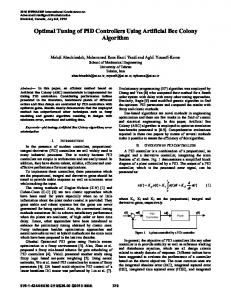
Using the method of Soylemez et al. (2003), the allowable range of K 3 is computed as [0.3, 97.0] by plotting K 3 versus θ (Fig. 2). The arbitrary value of K 3 = 70 is chosen in this range to obtain two singular values θ 1 = 0.836 and θ 2 = 1.449 from the figure. These values are substituted in (19) to obtain the equations of the CRB lines: K 1 + 1.34 K 2 − 30.73 = 0
(28)
K 1 + 0.24 K 2 + 232.71 = 0 The RRB inequalities are obtained as 2 K 2 + K 1 − 70 > 0
(29)
and 2 K 2 − K 1 + 3601.9 > 0
(30)
from (20) and (21), respectively. By plotting the boundaries (28), (29) and (30) in the K 1 − K 2 plane, the plane is divided into several domains (Fig. 3). The stability domain can be found by checking one arbitrary point in each domain. Using the inequalities (29) and (30), a smaller number of domains that satisfy these inequalities need to be checked. The stability domain is found as a triangle shown in Fig. 3. By incrementing K 3 and repeating the above procedure, different stability domains are obtained for each K 3 .The stability domains can then be visualized in a 3D plot as shown in Fig. 4. Now the 3D stability domain can be mapped to the space of the controller coefficients K P − K I − K D through the relationship (27). For a sampling period of T = 0.2 sec, the
mapping would be
7
2 K P − 1 − 2 K = 5 10 − 5 I K D 0 0.2 − 0.2
K1 K 2 K 3
The resulting 3D stability domain is shown in Fig. 5. 6. Discussions and Conclusions
In this paper, a method is presented for the evaluation of the allowable ranges of the variation of the coefficients of a digital PID controller to maintain stability. Simple linear equations are formed and then visualized in the space of controller coefficients to obtain the coefficient stability domains. The method is an extension of the parameter space results (Ackermann and Kaesbauer 2001) to the case of discrete-time PID control systems. An advantage of this method, due to the use of Jury’s test, is that the RRB is defined via inequalities rather than equalities. This specifies the stability domain more precisely and reduces the number of the domains to be checked for stability. The main advantage of the method of this paper over the approach of Keel et al. (2003) is the less computational requirement of this method. A comparison of the steps of the algorithm of Keel et al. (2003) and the algorithm presented here is given in Table 1. In the algorithm of Keel et al. (2003), it is required to multiply the characteristic equation by z – 1
N(z –1 ) which increases the order of the equation. For instance, to solve the example of
Section 5, the order will increase to 8 while the original characteristic equation is of order 5. Also, it is required to form 2n strings to check and validate the resulting inequalities. This number grows exponentially for higher order plants. For the example of Section 5, it is required to form 2 8 = 256 strings with the highest order of 8, and to apply the generalized Hermite-Biehler theorem for these strings to select the valid inequalities. These inequalities define the stability region in the K 1 − K 2 plane. The computational complexity of applying the generalized Hermite-Biehler theorem is also implied in Soylemez et al. (2003). On the other hand, the method of this paper gives the RRB explicitly in an analytic form via inequalities (20) and (21), and the CRB via equation (19). The requirement of computing the singular frequencies is common in the two algorithms. The extra requirement of the method presented here is the need for the stability checking of one point inside each region, formed by the root boundaries. The number of these regions is not large for arbitrary plants (see examples in Ackermann 2003). The inequalities (20) and (21) help to reduce the number of the regions need to be checked.
8
Further research on the computation of the admissible ranges of PID controller coefficients for achieving robust performance seems promising. Some works in this direction are presented in Ho and Lin (2003). Also, the recent developments of Gryazina and Polyak (2006) on the parameter space decomposition can be used to systematically evaluate the number of the regions need to be checked for the stability of PID control systems. References
J. Ackermann and D. Kaesbauer, “Design of robust PID controllers,” European Control Conference, pp.522-527, 2001. J. Ackermann, Robust Control: The Parameter Space Approach, Springer–Verlag, London, UK, 2002. K. Astrom, P. Albertos, and J. Quevedo, “PID Control,” Control Engineering Practice, pp.1159-1161, 2001. K. Astrom and T. Hagglund, PID Controllers: Theory, Design, and Tuning, Instrum. Soc. America, Research Triangle Park, NC, 1995. A. Datta, M.T. Ho, and S.P. Bhattacharyya, Structure and Synthesis of PID Controllers, Springer–Verlag, London, UK, 2000. J.F. Delansky and N.K. Bose, “Schur stability and stability domain construction,” Int. J. Control, Vol.49, No. 4, pp. 1175-1183, 1989. G.C. Goodwin, S.F. Graebe and M.E. Salgado, Control System Design, Prentice-Hall, Upper Saddle River, NJ, 2001. M.J. Grimble, Industrial Control Systems Design, John Wiley & Sons, Manchester, UK, 2001. E. N. Gryazina and B. T. Polyak, “Stability regions in the parameter space: D-decomposition revisited,” Automatica, vol. 42, pp.13-26, 2006. E.I. Jury and J. Blanchard, “A Stability test for linear discrete systems in table form,” IRE Proc., Vol. 49, No. 12, pp. 1947-1948, 1961. L.H. Keel, J.I. Rego, and S.P. Bhattacharyya, “A new approach to digital PID controller design,” IEEE Trans. Automatic Control, vol.48, No.4, 2003. M.T. Ho and C.Y.Lin, “PID Controller Design for roubust performance,”IEEE Trans. Automatic Control, vol.48, pp.1404-1409, 2003. K. Ogata, Discrete Time Control Systems, Prentice-Hall, Englewood Cliffs, NJ, 1994. M. T. Soylemez, N. Munro and H. Baki, “Fast calculation of stabilizing PID controllers,” Automatica, pp.121-126, 2003. H. Xu, A. Datta and S.P. Bhattacharyya, “Computation of all stabizing PID gains for digital control systems,” IEEE Trans. Automatic Control, vol.46, No.4, 2001.
9
Table 1. A comparison of the algorithms of Keel et al. (2003) and this paper. step
Method of Keel et al. (2003)
Method of this paper
1
Multiplying the characteristic equation by Computing singular frequencies z –1 N(z –1 ) and decomposing it into two real from (18). and imaginary parts.
2
Solving the imaginary part of the equation for Compute the CRB and the RRB finding singular frequencies. boundaries from (19), (20) and (22).
3
Check one point inside each feasible Forming 2n possible strings for testing, where region formed from the intersection n is the number of singular frequencies. of the lines defined in step (2).
4
Substituting the singular frequencies in the real part to obtain a set of linear inequalities.
5
Finding the valid linear inequalities among the inequalities of step (4), using the generalized Hermite-Biehler theorem by checking the strings formed in step (3).
10
R(z) +
C(z)
G(z)
Y(z)
-
Fig. 1. Digital feedback control system.
Fig. 2. Plotting K3 versus θ for the example.
Fig. 3. Stability domain in the K1-K2 plane (The black triangle).
11
Fig. 4. Stability domain in the K1-K2-K3 space.
Fig. 5. Stability domain in the KP-KI-KD space.
12