design of efficient synchronization protocols for ...

AFRL-RI-RS-TR-2008-197 Final Technical Report July 2008

DESIGN OF EFFICIENT SYNCHRONIZATION PROTOCOLS FOR WIRELESS AIRBORNE NETWORKS Texas A & M University

APPROVED FOR PUBLIC RELEASE; DISTRIBUTION UNLIMITED.

STINFO COPY

AIR FORCE RESEARCH LABORATORY INFORMATION DIRECTORATE ROME RESEARCH SITE ROME, NEW YORK

NOTICE AND SIGNATURE PAGE

Using Government drawings, specifications, or other data included in this document for any purpose other than Government procurement does not in any way obligate the U.S. Government. The fact that the Government formulated or supplied the drawings, specifications, or other data does not license the holder or any other person or corporation; or convey any rights or permission to manufacture, use, or sell any patented invention that may relate to them. This report was cleared for public release by the Air Force Research Laboratory Public Affairs Office and is available to the general public, including foreign nationals. Copies may be obtained from the Defense Technical Information Center (DTIC) (http://www.dtic.mil). AFRL-RI-RS-TR-2008-197 HAS BEEN REVIEWED AND IS APPROVED FOR PUBLICATION IN ACCORDANCE WITH ASSIGNED DISTRIBUTION STATEMENT.

FOR THE DIRECTOR: /s/

GREGORY HADYNSKI Work Unit Manager

/s/

WARREN H. DEBANY, JR Technical Advisor Information Grid Division

This report is published in the interest of scientific and technical information exchange, and its publication does not constitute the Government’s approval or disapproval of its ideas or findings.

Form Approved

REPORT DOCUMENTATION PAGE

OMB No. 0704-0188

Public reporting burden for this collection of information is estimated to average 1 hour per response, including the time for reviewing instructions, searching data sources, gathering and maintaining the data needed, and completing and reviewing the collection of information. Send comments regarding this burden estimate or any other aspect of this collection of information, including suggestions for reducing this burden to Washington Headquarters Service, Directorate for Information Operations and Reports, 1215 Jefferson Davis Highway, Suite 1204, Arlington, VA 22202-4302, and to the Office of Management and Budget, Paperwork Reduction Project (0704-0188) Washington, DC 20503.

PLEASE DO NOT RETURN YOUR FORM TO THE ABOVE ADDRESS. 1. REPORT DATE (DD-MM-YYYY) 2. REPORT TYPE

JUL 2008

3. DATES COVERED (From - To)

Final

MAR 07 – JAN 08

4. TITLE AND SUBTITLE

5a. CONTRACT NUMBER

DESIGN OF EFFICIENT SYNCHRONIZATION PROTOCOLS FOR WIRELESS AIRBORNE NETWORKS

5b. GRANT NUMBER

FA8750-07-1-0061 5c. PROGRAM ELEMENT NUMBER

62702F 6. AUTHOR(S)

5d. PROJECT NUMBER

CITE Erchin Serpedin

5e. TASK NUMBER

TE 5f. WORK UNIT NUMBER

XS 7. PERFORMING ORGANIZATION NAME(S) AND ADDRESS(ES)

8.

Texas A & M University 1470 William d Fitch PKWY College Station, TX 77845-4645

PERFORMING ORGANIZATION REPORT NUMBER

9. SPONSORING/MONITORING AGENCY NAME(S) AND ADDRESS(ES)

10. SPONSOR/MONITOR'S ACRONYM(S)

AFRL/RIGC 525 Brooks Rd Rome NY 13441-4505

11. SPONSORING/MONITORING AGENCY REPORT NUMBER

AFRL-RI-RS-TR-2008-197

12. DISTRIBUTION AVAILABILITY STATEMENT

APPROVED FOR PUBLIC RELEASE; DISTRIBUTION UNLIMITED. PA# WPAFB 08-08-3811

13. SUPPLEMENTARY NOTES

14. ABSTRACT

The goal of this project was to develop efficient clock synchronization schemes to ensure robust operation of wireless airborne networks in the absence of GPS (Global Positioning Systems), and in the presence of mobility, time-varying channel conditions, and ad-hoc network topologies. The major contributions of this project include the development of analytical performance tools to assess the performance of clock synchronization protocols and development of novel clock synchronization protocols to achieve the ultimate performance limits predicted by the analytical performance benchmarks. The work conducted in this project lead also to the development of two novel time synchronization protocols: Adaptive Synchronization Protocol and Pairwise Broadcast Synchronization (PBS) Protocol, respectively, which were shown to exhibit a number of desirable features (such as scalability, adaptivity, energy-efficient and distributed capabilities) for clock synchronization in wireless airborne networks and wireless sensor networks. 15. SUBJECT TERMS

Wireless airborne networks, network protocols, time synchronization

17. LIMITATION OF ABSTRACT

16. SECURITY CLASSIFICATION OF: a. REPORT

U

b. ABSTRACT

U

c. THIS PAGE

U

UU

18. NUMBER OF PAGES

51

19a. NAME OF RESPONSIBLE PERSON

Gregory Hadynski 19b. TELEPHONE NUMBER (Include area code)

315-330-4094 Standard Form 298 (Rev. 8-98) Prescribed by ANSI Std. Z39.18

Contents 1 Summary

1

2 Introduction

3

3 Methods, Assumptions and Procedures

6

4 Results and Discussion

9

4.1

Efficient Clock-Offset Compensation Schemes for Local Network Synchronization .

4.2

Adaptive-Sync Protocol for Global Network Synchronization . . . . . . . . . . . . 16 4.2.1

4.3

9

Number of Beacons Required for Each Pairwise Synchronization . . . . . . 22

Pairwise Broadcast Synchronization (PBS) Protocol . . . . . . . . . . . . . . . . . 23 4.3.1

Pairwise Sender-Receiver Synchronization . . . . . . . . . . . . . . . . . . 25

4.3.2

Receiver-Only Synchronization . . . . . . . . . . . . . . . . . . . . . . . . . 27

4.3.3

Receiver-Receiver Synchronization . . . . . . . . . . . . . . . . . . . . . . . 29

4.3.4

Comparisons and Analysis . . . . . . . . . . . . . . . . . . . . . . . . . . . 32

5 Conclusions

34

6 List of Symbols, Abbreviations, and Acronyms

41

7 List of Publications Resulted from this Project

43

ii

List of Figures 1

a) Message exchange between master-slave nodes having clock offset. b) Message exchange between master-slave nodes having clock offset and skew.

2

. . . . . . . . 11

a) Variance of MLE for the Gaussian delay model and the proposed estimator for Gaussian random delays (σ 2 = 1). b) Variance of MLE for the Gaussian delay model and the proposed estimator for exponential random delays (α = 1). . . . . . 13

3

Required number of message exchanges with respect to the number of sensor nodes. 23

4

Receiver-only synchronization. . . . . . . . . . . . . . . . . . . . . . . . . . . . . . 24

5

Clock synchronization model of PBS. . . . . . . . . . . . . . . . . . . . . . . . . . 26

6

Performance of PBS clock offset and skew estimation. . . . . . . . . . . . . . . . . 30

7

Receiver-receiver synchronization. . . . . . . . . . . . . . . . . . . . . . . . . . . . 31

8

Clock synchronization model of RBS. . . . . . . . . . . . . . . . . . . . . . . . . . 33

iii

Acknowledgements The PI would like to express his heartfelt thanks to Mr. Gregory Hadynski and Dr. Bruce Suter from Air Force Research Laboratory (AFRL), Rome, NY, for all their support, help and encouragement.

iv

1

Summary

The main goal of this project was to develop efficient clock synchronization schemes to ensure robust operation of wireless airborne networks in conditions of mobility, time-varying channel conditions, ad-hoc decentralized infrastructures and absence of GPS (Global Positioning Systems). To achieve this goal, a number of tasks were accomplished in this project. The first task dealt with in this project was the development of analytical performance benchmarks to assess the performance of clock synchronization protocols for wireless ad-hoc networks at micro-level, i.e., sub-networks involving the synchronization of two or a limited number of adjacent nodes. This first task was fully addressed in this project, and efficient analytical tools to assess the performance of clock synchronization algorithms in terms of the Cramer-Rao lower bound (CRLB) and mean-square error (MSE) were developed. The second task of this project focused on designing efficient and robust clock synchronization algorithms that achieve these ultimate performance limits, and on validating the performance of these algorithms through computer simulations. The second task was also successfully addressed in this project. Finally, the third major task of this project was the design of energy-efficient protocols for synchronization of large-scale wireless ad-hoc airborne networks. Two novel protocols entitled Adaptive-Sync Protocol and PBS (Pairwise Broadcast Synchronization) Protocol, respectively, were developed for synchronization of large-scale wireless airborne networks and shown to exhibit all the desirable features: scalability, distributivity, adaptivity, energy-efficiency, decentralized operation, and ability to perform local as well as global synchronization. The work conducted in this project was reported in numerous journal and conferences, and in several PhD and MSc Thesis Dissertations at Texas A&M University that are publicly available. Overall, this project lead to a large number of novel results of paramount importance in the area of clock synchronization of wireless ad-hoc networks and more

1

general networks such as Internet. Some of these results could be viewed as real breakthroughs. As examples of such breakthrough results, this project developed clock synchronization schemes that achieve the ultimate performance limits, outperform significantly the existing state-of-theart schemes and are robust to the distribution of network delays. High-performance extensions of the most representative protocols RBS (Reference Broadcast Synchronization) and TPSN (Timing Synch Protocol for Sensor Networks) proposed for clock synchronization of wireless ad-hoc (sensor) networks were also derived. The proposed PBS and Adaptive-Sync protocols represent high-performance energy-efficient extensions of RBS and TPSN protocols, respectively.

2

2

Introduction

Future wireless airborne networks are envisioned to represent the next frontier of networking, to be pervasive and ubiquitous, and to provide a wide range of services and applications. This trend is underlined by a number of technological advances and demands. The rapidly growing demands for mobility and anywhere-anytime data access represents a major driving force behind the next generation of mobile wireless airborne networks. Recent technological developments mark also the departure of telecommunications systems from homogeneous networks to heterogeneous networks, from non-intelligent devices to smart devices, and from telephony-based services to multi-media services. In addition, recent advances in hardware and inexpensive wireless radio systems have made also possible the design of low-cost, low-power, and multi-functional sensor devices. When deployed in a large number across a geographical area, these sensor devices create a self-organized cooperative ad-hoc network that is perfectly fit for distributed sensing and automated information gathering, processing and communication. Wireless sensor networks have been recognized as a revolutionary technology that will have a huge impact on a broad range of applications: monitoring the health status of humans and environment, control and instrumentation of industrial machines and home appliances, energyconservation, security, detection of chemical and biological leaks, etc. Wireless sensor networks are a special case of wireless ad hoc networks, and assume a multi-hop communication framework with no infrastructure and where the sensors cooperate spontaneously by forwarding each other’s packets from a source to a destination node. The upcoming years will very likely witness a growing demand for more intelligent sensor systems that will be networked with wireless local area networks (WLANs), Internet, satellite and Unmanned Aerial Vehicle (UAV) networks to create a global wireless airborne network with increased functionality and performance.

3

In general, for distributed computing and networking systems, maintaining the logical clocks of the computers in such a way that they are never too far apart is one of the most complex problems of computer engineering. Whether it is the disciplining of computer clocks with the devices synchronized to a Global Positioning System (GPS) satellite or a Network Time Protocol (NTP) time server over the Internet, it is possible to equip some primary time servers for the purpose of synchronizing a much larger number of secondary servers and clients connected through a common infrastructure. In order to do this, a distributed network clock synchronization protocol is required through which a server clock can be read, the readings to other clients can be transmitted and each client clock can be adjusted as required. In such a distributed synchronization approach, the participating devices exchange timing information with their chosen reference at regular intervals and adjust their logical clocks accordingly. A computer clock in general has two components, namely a frequency source and a means of accumulating timing events (consisting of a clock interrupt mechanism and a counter implemented in software). The implementation of the computer clock in the operating system and the programming interface differ between operating systems and hardware platforms. However, the basic source of timing are an uncompensated quartz crystal oscillator and the clock interrupts it generates. Theoretically, two clocks would remain synchronized if their offsets are set equal and their frequency sources run at the same rate. However, practical clocks are set with limited precision and the frequency sources run at slightly different rates. In addition, the frequency of a crystal oscillator varies due to initial manufacturing tolerance, aging, temperature, pressure and other factors. Because of these inherent instabilities, distributed clocks must regularly be synchronized to keep them running close to each other. The Network Time Protocol [23] represents the most widely used clock synchronization protocol for large-scale networks with static topology such as the Internet. In NTP, the nodes are 4

externally synchronized to a global reference time that is represented in the network by a set of master nodes or time servers that are referred to as layer-1 servers. The entire synchronization process assumes a hierarchical tree organization of the network nodes. Despite its wide-spread use in the synchronization of Internet, NTP is not appropriate for synchronization of wireless ad-hoc sensor networks that are subject to severe energy-constraints, dynamic topologies caused by mobility and node failures, and absence of GPS and global time references (due to either jamming, interferences, or absence of direct line of sight communication links). In addition, the service provided by NTP assumes continuous synchronization of all the network nodes with maximum accuracy and with no concern about energy consumption. However, NTP is not equipped with an mechanism to enable the local synchronization of a subset of nodes, and to keep the rest of the nodes switched to a power-saving (sleeping) state. Since listening continuously for the synchronization beacons is an energy-consuming operation, NTP can not directly be applied to synchronization of energy-constrained wireless ad-hoc networks as is the case with wireless airborne networks and wireless sensor networks. These considerations illustrate the need for novel distributed and scalable synchronization protocols for wireless ad-hoc networks that in general must satisfy a series of requirements: energy-efficiency, robustness with respect to node mobility and link/node failures, and ability to guarantee the long-term network synchronization at local and global scales. Clock synchronization is important for many applications such as Internet delay measurements, cellular networks, data security algorithms, Media Access Control (MAC) protocols like Time Division Multiple Access (TDMA), Internet Protocol (IP) telephony, ordering of updates in database systems, etc. Recently, with the advent of Wireless Sensor Networks (WSNs) and Wireless Airborne Networks (WANs), developing clock synchronization protocols that suit their specific requirements is becoming an important research problem [30]. A large number of their 5

applications require the clocks of the nodes to run synchronously on a common timescale. This is the case with applications such as data fusion, efficient duty cycling operations, acoustic beamforming, localization, security and object tracking. Unlike conventional networks, energy efficiency must also be taken into account for addressing the clock synchronization problem in WSNs and WANs.

3

Methods, Assumptions and Procedures

During the last two decades, many clock synchronization protocols have been proposed such as [4], [5], [23], etc. NTP [23] is a protocol for synchronizing the clocks of computer systems over packet-switched, variable-latency data networks and it represents the Internet standard for time synchronization. It is a layered client-server architecture based on the User Data Protocol (UDP) message passing which synchronizes computer clocks in a hierarchical way using the offset delay estimation method. NTP’s sender-receiver synchronization architecture is widely accepted in designing time synchronization algorithms and consists of the same two-way timing message exchange mechanism targeted in this paper. A protocol based on the remote clock reading method was put forward by [5], which handles unbounded message delays between processes. In [4], the time transmission protocol is used by a node to communicate the time on its clock to a target node, which subsequently estimates the time in the source node by using message timestamps and message delay statistics. For ad-hoc communication networks, the time synchronization protocol [28] represented one of the pioneering contributions in this area. The protocol is based on generating timestamps to record the time at which an event of interest occurred. The timestamps are updated by each node using its local clock and the time transformation method, where the final timestamp is

6

expressed in terms of an interval with a lower bound and an upper bound. In the realm of wireless sensor networks, the clock synchronization protocols of particular note are Reference Broadcast Synchronization (RBS [7]), Timing Synch Protocol for Sensor Networks (TPSN [8]) and Time Diffusion Protocol (TDP [21]). RBS relies on simultaneous reception of broadcast pulses by several nodes transmitted by a common neighboring node after which the nodes exchange their timestamps and estimate the relative time offsets and skews. On the other hand, TPSN is based on the same sender-receiver paradigm as in NTP, like many other traditional clock synchronization protocols. The basic difference is that TPSN has been molded sufficiently to suit the requirements of wireless sensor networks. On the other side, TDP establishes a network-wide equilibrium time through an iterative, weighted averaging technique based on a diffusion of messages involving all the nodes in the synchronization process. In general, there are two different approaches for synchronizing a pair of nodes which can be categorized as sender-receiver synchronization (SRS) and receiver-receiver synchronization (RRS). The former is based on the classical model of two-way message exchanges between a pair of nodes. In contrast, the latter compares the time readings of a beacon packet from a common sender at a set of nodes. Most of the existing time synchronization protocols rely on one of these two approaches. For instance, RBS is based on RRS since it requires pairs of message exchanges among children nodes (except the reference) to compensate their relative clock offsets, while TPSN adopts SRS since it depends on a series of pairwise synchronizations that assume two-way timing message exchanges. The work conducted in this project focused in the following main directions: • development of a comprehensive body of analytical results to assess the ultimate performance limits achievable by clock synchronization protocols, and design of energy-efficient

7

protocols to achieve these limits. • development of energy efficient protocols for global synchronization of wireless ad-hoc (sensor) networks. • design of synchronization schemes that are robust to the high-latencies induced by large propagation delays, clock skew variations, and network traffic delays. This research work plays a fundamental role in the design of future generation of energy-efficient long-lived wireless airborne networks. The studies offered by current protocols (RBS [7], TPSN [8], Flooding Time Synchronization Protocol (FTSP) [22], tiny/mini synchronization [32], diffusion algorithm [21], etc.) have concentrated on short-term and small-scale sensor network synchronization, and are not fit for synchronization of long-term and large-scale networks that require efficient duty-cycling mechanisms in the presence of continuous time synchronization (e.g., coordinated actuation and synchronized sampling) and/or sensor-initiated (post-facto) synchronization. The lack of techniques to accurately predict the performance of time synchronization protocols has been recently recognized as an important obstacle in designing long-lived wireless sensor networks. By eliminating the empiric and highly suboptimal design principles used in the current synchronization protocols, the design principles established in this project will help reduce dramatically the re-synchronization rate, reduce the signaling rate and transmission packet overhead, optimize the operation of existing synchronization protocols, and help in establishing the foundations for the design of future generation of long-lived energy-efficient sensor networks. One of the major benefits of the work conducted in this project is the development of the energy-efficient Adaptive-Sync and PBS (Pairwise Broadcast Synchronization) protocols for long-term synchronization of sensor networks. The Adaptive-Sync Protocol exhibits a number of very attractive features for synchronization of sensor networks: 8

• it represents a significantly enhanced and natural extension of NTP and TPSN for global synchronization of large-scale ad-hoc networks • it aims at minimizing the energy consumption in large-scale and long-lived sensor networks • it is equipped with flexible mechanisms to adjust the synchronization mode (local versus global), (re-) synchronization period, and clock phase-offset and skew estimators in order to achieve long term reliability • it employs sequential message exchange techniques and energy-efficient signaling schemes to reduce further the number of RF-transmissions • as opposed to RBS, TPSN, and FTSP protocols that perform poorly in high-latency networks, the Adaptive-Sync Protocol is also fit for networking environments characterized by high propagation delays and clock skew variations, and exhibits robustness to unknown network delay distributions.

4

Results and Discussion

In the present section, we will discuss the major results that were accomplished in this project.

4.1

Efficient Clock-Offset Compensation Schemes for Local Network Synchronization

The very first step in designing an efficient synchronization protocol is to develop efficient schemes for pairwise synchronization of two nodes, and to understand what are the ultimate performance limits and to design estimation schemes that achieve these limits. From the theory of point estimation [19], it is known that once an analytical model is available for a given estimation method, then under some general conditions, a lower bound for the variance of any unbiased 9

estimator can be expressed in terms of the Cramer-Rao lower bound (CRLB). Furthermore, techniques to build estimators that achieve the ultimate performance predicted by Cramer-Rao lower bound are available (e.g., the maximum likelihood estimation principle, the Rao-Blackwell and Lehmann-Scheffe constructions of minimum variance unbiased estimators) [19], [15]. These were the basic ideas that this project followed to assess the ultimate performance of existing synchronization schemes and to develop synchronization schemes that achieve these performance limits. The common synchronization protocols NTP and TPSN rely on the clock offset correction scheme between two nodes that assumes the pairwise message exchange mechanism depicted in Fig. 1. Since the NTP and TPSN protocols assumes no clock skew (frequency offset) between the two nodes, we will improve by a significant margin the performance of NTP and TPSN protocols by the introduction of a clock skew correction mechanism within the same message exchange protocol and without causing any additional overhead. First we will derive the maximum likelihood estimator (MLE) and the Cramer-Rao lower bound for the clock phase-offset in the presence of Gaussian network delays and no clock skew, and then address the issue of clock skew compensation. Assume that the message exchanges that take place between two generic nodes A and B are the ones depicted in Fig. 1-a. Node A sends its time reading T1,i to Node B, which records its time of arrival T2,i according to its own timescale. A similar timing message exchange is sent from Node B to Node A. The ith delay observations corresponding to the ith timing message exchange are given by Ui = d + θA + Xi and Vi = d − θA + Yi , respectively (using similar notations as in [1]), and are graphically represented in Fig. 1-a. The fixed value θA denotes the clock offset between the two nodes, Xi and Yi denote the variable portions of delays which are assumed to be normal distributed random variables (RVs) with mean µ and variance σ 2 , respectively. 10

θ A : clock offset (time difference) θ B : clock skew (frequecy difference) T2,i

node B

θ B (T1,i + d + X i )

T3,i

θ B (T4,i − d − Yi )

Node B

T2,1 T3,1

T2,N

T2,i T3,i

T3,N

θ B (T4, N − T1,1 )

T2,2 T3,2

θ A( R )

Node A node A

T1,i Ui = d + θ A + X i

( R) T1,1( R ) T4,1 T1,2( R )

T4,i

(R) T4,2

T1,(iR )




T1, i = T1,(iR ) − T1,1( R )

Vi = d − θ A + Yi

d + Xi

T4,( Ri )

T1,( NR )




T4,( RN)

d + Yi

T4, i = T4,( Ri ) − T1,1( R )

T1,1 = 0

Figure 1: a) Message exchange between master-slave nodes having clock offset. b) Message exchange between master-slave nodes having clock offset and skew.

N Maximizing the likelihood function based on the observations {Xi }N i=1 and {Yi }i=1 , we arrive at

the MLE of clock offset: N P

θˆA = arg max [ln L (θA )] = θA

(Ui − Vi )

i=1

2N

=

U −V , 2

(1)

N where U and V stand for the sample means of observations {Ui }N i=1 and {Vi }i=1 , respectively.

The CRLB of estimator (1) takes the form: σ2 . var(θˆA ) ≥ CRLB(θˆA ) = 2N

(2)

The computer simulations illustrate that the mean-square error (MSE) of MLE (1) is well predicted by the CRLB (2) for any number of observations N (see Fig. 2-a). It is interesting to observe that the expression and performance of MLE strongly depends on the type of distribution assumed by network delays (see Fig. 2-b). We have shown (see the references [27], [31]) that when the network delays are exponentially distributed with mean α, the MLE and corresponding

11

CRLB for the clock phase offset assume the expressions: θˆA =

min Ui − min Vi

1≤i≤N

1≤i≤N

2

var(θˆA ) ≥ CRLB(θˆA ) =

,

(3)

α2 . 4N 2

(4)

Extensive computer simulations illustrate that the performance of MLEs (1) and (3) is not robust with respect to (wrt) the network delay distribution. In other words, the Gaussian MLE (1) and exponential MLE (3) perform very poorly in the presence of exponential and Gaussian network delays, respectively. Notice that this disproportionate behavior is corroborated by the totally different dependence of CRLBs (2) and (4) with respect to the number of observations N (linear vs. quadratic). This suggests the need for robust estimation schemes that exhibit good performance irrespective of the underlying distribution of network delays. Our preliminary computer simulation results (see our preliminary publication [18]) show that the clock-offset estimators built within the framework of sequential Markov-Chain Monte-Carlo techniques are robust with respect to the distribution of network delays and present excellent performance.

Next, based on the same pairwise message exchange mechanism, we will develop a novel approach to compensate both the clock phase offset as well as the skew. Since every oscillator has its unique clock frequency, the clock offset between two nodes generally keeps drifting away. Also, since a fixed value model for clock offset is not sufficient, estimating the difference of clock frequencies (i.e., clock skews) between two nodes increases the synchronization accuracy and guarantees long-term reliability without frequent re-synchronization. We will next illustrate the main challenges behind determining efficient joint ML-estimators for clock phase and skew offset, and then show a technique to build high-performance estimators for clock-phase and skew offset that are robust to high-latencies (unknown possible large propagation delays). Due to 12

α=1

Exponential Delay Model

−3

σ=1

Gaussian Delay Model

−3

10

EMLLE (unknown d) GMLE (known d) Lower Bound for EMLLE

10

GMLLE (unknown d) GMLE (known d) Lower Bound for GMLLE CRLB −4

10 −4

Variance

Variance

10

−5

10 −5

10

−6

10 −6

10

5

10

15 20 25 Number of Observation

30

5

10

35

15 20 25 Number of Observations

30

35

Figure 2: a) Variance of MLE for the Gaussian delay model and the proposed estimator for Gaussian random delays (σ 2 = 1). b) Variance of MLE for the Gaussian delay model and the proposed estimator for exponential random delays (α = 1). space limitations, we will only sketch the main results. Fig. 1-b shows the effect of clock skew (denoted by θB ) on the timing message exchange between the two nodes A and B. In this model, the ith received signal at the node B, T2,i , is given by T2,i = T1,i + d + Xi + θB (T1,i + d + Xi ) + θA = (1 + θB ) (T1,i + d + Xi ) + θA ,

(5)

where the additional term θB (T1,i + d + Xi ) is due to the effect of clock skew. Similarly, the ith received signal at the node A, T4,i , is expressed as T4,i = T3,i + d + Yi − θB (T4,i − d − Yi ) − θA ,

(6)

T3,i = (1 + θB ) (T4,i − d − Yi ) + θA ,

(7)

where the term θB (T4,i − d − Yi ) is again due to the drift caused by clock skew, and (7) is N obtained by re-arranging (6). Assuming that {Xi }N i=1 and {Yi }i=1 are zero mean independent

Gaussian distributed RVs with variance σ 2 , and the fixed portion of delay d is known, the Maximum Likelihood (ML) estimates for θA and θB can be expressed in closed-form as a function of unknown delay parameter d (a result derived in more details in our publication [27]). Notice 13

further that in general framework networks that rely on Radio Frequency (RF) transmissions over short distances, d can be assumed known (d = 0), and the proposed MLEs of clock phase-offset and skew are directly implementable. Since the clock difference between two wireless terminals is monotonically increasing or decreasing due to the linear clock skew model, the clock difference will be maximized between the first and last time stamps. From this intuition, novel and practical clock skew estimators can be developed by using the first and last observations of timing message exchanges. The idea is to build clock skew estimates that maximize the likelihood function based on the first and last observations of timing stamps. From (5), subtracting T2,1 from T2,N gives T2,N − T2,1 = T1,N − T1,1 + XN − X1 + θB (T1,N − T1,1 + XN − X1 ) .

(8)

Similarly from (6), subtracting T4,1 from T4,N yields T4,N − T4,1 = T3,N − T3,1 + YN − Y1 − θB (T4,N − T4,1 − (YN − Y1 )) . Define the differences of the first and last time stamps as D(1) = D(2) =

PN

i=2 D2,i

= T2,N −T2,1 , D(3) =

PN

i=2 D3,i

PN

= T3,N −T3,1 , and D(4) =

i=2 D1,i

PN

(9)

= T1,N − T1,1 ,

i=2 D4,i

= T4,N −T4,1 ,

respectively, and where Dk,l = Tk,l − Tk,l−1 captures the difference between two consecutive time stamps (k = 1, . . . , 4, l = 2, . . . , N ). Then, (8) and (9) can be rewritten respectively as ¡ ¢ D(2) = D(1) + P + θB D(1) + P , ¡ ¢ D(4) = D(3) + R + θB D(4) − R , where P = XN − X1 and R = YN − Y1 . Since XN , X1 , YN , and Y1 are i.i.d. (independent and identically distributed) normal distributed RVs with variance σ 2 , P and R are zero-mean normal distributed RVs with variance 2σ 2 , respectively. So the joint Probability Density Function (PDF)

14

of P and R is given by

µ fP,R (p, r) =

1 4πσ 2

¶2

e− 4σ2 (p 1

2 +r 2

).

0 = 1/(1 + θB ) and σ 2 takes the form The likelihood function with respect to θB

¡ 0 2¢ L θB ,σ =

µ

1 4πσ 2

¶2

−

e

1 4σ 2

h i 2 2 2 2 D(2) (θB0 −β ) +D(3) (θB0 −γ )

,

(10)

0 and by maximizing (10) with respect to θB leads to the clock-skew estimator: 2 2 + D(3) D(2) 1 ˆ θB = −1= − 1. 0 D(1) D(2) + D(3) D(4) θˆB

(11)

This analysis can be further extended to derive efficient clock-skew estimators in the case of exponentially distributed latencies. Notice further that the proposed clock-skew estimator (11) can be used to determine efficient clock phase-offset estimators. Using (5) and (6), the ith observations of timing message exchange delays Ui = T2,i − T1,i and Vi = T4,i − T3,i are expressed, respectively, as Ui = d + Xi + θB (T1,i + d + Xi ) + θA , Vi = d + Yi − θB (T4,i − d − Yi ) − θA . Since T2,i and T4,i are known values and θB can be estimated (11), the sets of delay observations between the two nodes can be recomposed as Ui0 = Ui − θˆB T1,i

(= d0 + θA + Xi0 ) ,

(12)

Vi0 = Vi + θˆB T4,i

(= d0 − θA + Yi0 ) ,

(13)

where Xi0 = (1 + θB ) Xi , Yi0 = (1 + θB ) Yi , and d0 = (1 + θB ) d, respectively. Since the clock-skew is compensated, eqs. (12) and (13) suggest that the same ML clock offset estimators as in (1) and (3) for Gaussian and exponential delay models, respectively, can be applied to arrive at the 15

estimates: Ui0 − Vi0 θˆA = 2 min Ui0 − min Vi0 1≤i≤N 1≤i≤N θˆA = 2

(Gaussian delays),

(14)

(exponential delays).

(15)

Fig. 2-a compares the MSEs of the proposed clock-skew estimator (11) for the Gaussian delay model with MLE (that assumes knowledge of d) and corresponding CRLB in Gaussian random delay channels (σ 2 = 1). It can be seen that the proposed estimator (11) performs close to MLE, is consistent and asymptotically efficient. Fig. 2-b shows the variance of the counterpart estimator (11) for the exponential delay model and that of MLE (that assumes knowledge of d) for the Gaussian delay model in exponential random delay channels (α = 1). It can also be seen that the proposed estimator is consistent and exhibits comparable performance to the ideal MLE.

4.2

Adaptive-Sync Protocol for Global Network Synchronization

The work conducted in this project also lead to the development of a significantly enhanced extension (named Adaptive-Sync Protocol) of NTP and TPSN protocols. Adaptive-Sync adaptively optimizes some crucial network parameters, such as the synchronization mode, the resynchronization period and the number of beacons per pairwise synchronization, with respect to the current network status. The Adaptive-Sync Protocol consists of three functional phases: • Level discovery phase: This phase is the same as that in TPSN, and is used for generating a hierarchical structure in the network. • Synchronization phase: It is similar to the corresponding synchronization phase in TPSN. However, as opposed to TPSN, the Adaptive-Sync Protocol adjusts not only the current 16

clock offset but also the clock skew to guarantee the long term synchronization, while TPSN only estimates the clock offset. Hence, the Adaptive Sync Protocol requires far less frequent re-synchronization. • Network evaluation phase: The reference node investigates the current status of network traffic in order to select the synchronization mode between always on (AO) (always maintain network-wide synchronization) and sensor initiated (SI) (synchronize only when it needs to). Besides, it optimizes the re-synchronization period and the number of beacons per each pairwise synchronization. The second and third phases (i.e., synchronization and the network evaluation phases) will be periodically repeated in order to minimize the overall energy consumption with respect to the current network status. The Adaptive-Sync Protocol assumes also a number of additional parameters such as latency factor, average number of hops, and timing synchronization period to optimize the overall performance of synchronization protocol. Relative to TPSN protocol, Adaptive-Sync assumes the additional network evaluation phase, while the functions of the other two phases present some common similarities with the ones encountered in TPSN. In the synchronization phase, Adaptive-Sync estimates not only the current clock drift but also the clock frequency (skew) to guarantee long term reliability of synchronization while TPSN only estimates the clock offset, and therefore TPSN might require more frequent network-wide synchronization. Robustness to high-latencies and distribution of network delays is ensured based on the clock estimators presented in the previous section. Furthermore, Adaptive-Sync adapts the clock offset and skew estimators in order to achieve long term synchronization. As TPSN, generating a hierarchical structure in the network, the level discovery phase, is the first step of Adaptive-Sync. In this phase, every single node in the network will be assigned a

17

level and gets ready for synchronization. Upon creating the network hierarchy, the reference node investigates the current status of network traffic in order to adjust the period of synchronization and select the synchronization mode between always on (AO - always maintain network-wide synchronization) and sensor initiated (SI - synchronize only when it needs to). This step stands for the network evaluation phase, and its goal is to minimize the number of message exchanges for synchronization in a given time interval, i.e., it aims to minimize total energy consumption for synchronization. The third step of Adaptive-Sync, called network-wide time synchronization, consists in the pairwise synchronization between adjacent nodes until every node in the network is synchronized to the reference(s). Adaptive-Sync periodically repeats the network evaluation and synchronization phases to minimize the total energy consumption in the network with respect to the current network status. Another critical problem is to determine the required number of timing message exchanges per each pairwise synchronization. To achieve higher synchronization accuracies, a larger number of message transfers and an additional signal processing workload are needed during each pairwise synchronization. As the number of required timing messages per each pairwise synchronization increases, the overall number of timing messages in a synchronization period increases. Hence, there is a tradeoff between accuracy and energy consumption. To address these design challenges, next we propose an adaptive clock synchronization algorithm to aid in selecting the synchronization mode between AO and SI, the period of synchronization τ , and the number of message exchanges per pairwise synchronization N aiming at efficient usage of network resources for reduced energy consumption. The network parameters are summarized as follows: • B: number of branches in a spanning tree of the network. • τ : period of clock synchronization.

18

• h: average number of hops per unit time • δ: latency factor reflecting the amount of allowed delay in data transmission • N : number of message exchanges per pairwise synchronization The number of branches in the network B can be obtained after the level discovery phase. The latency factor δ should be fixed according to the type of sensor network and its range is from 0 to 1. The higher latency factor means higher concern for network delays. In every sensing event, the destination node adds the number of hops that have occurred in that particular transmission to its storage. During the next synchronization phase, the reference node collects the information of the total number of hops occurred in the last sync period and determines the average number of hops per unit time (h) in the network. As mentioned earlier, the goal of the adaptive clock synchronization algorithm is to minimize the number of required timing messages. In an AO-mode, the number of timing messages per unit time is given by M = 2BN/τ , while in the SI-mode, M = 2hN . To minimize the number of timing messages per unit time M , the synchronization mode should be selected as follows: 2BN δ AO ≶ 2hN, τ SI

(16)

where the latency factor δ varies from 0 to 1 such that the more delay-dependent networks assume a larger value of δ and vice versa (0 ≤ δ ≤ 1). For example, δ is set to 0 for sensor networks requiring network synchronization all the time (only AO mode is available). On the other extreme, for delay-independent networks, δ should be close to 1. As the period of timing synchronization τ is getting larger, the network is getting power efficient. Thus, τ should be chosen as large as possible. However, a too large value for τ induces a critical synchronization problem since the clock drift between nodes keeps generally increasing with time. Hence, there exists a maximum value of timing sync period (τ = τmax ) 19

which is determined by the oscillator characteristics (hardware specifications) and the accuracy of estimators. Notice that (16) can be rewritten as AO

τmax ≷ SI

Bδ (= Th ). h

(17)

Thus, the sync mode changes from AO into SI when Th is greater than τmax . In the SI-mode, the reference node periodically asks the number of hops that occurred during the past time interval, and then make a decision whether or not to switch to the AO-mode. In fact, τmax is dependent on N since it strongly depends on the accuracy of timing offset estimators. A more detailed analysis of τmax is provided next. The synchronization phase performs pairwise synchronization among a set of nodes by exchanging timing messages. For the AO-mode, a series of pairwise synchronization will take place until every node in the network is synchronized to the reference node, i.e., the message exchanges are occurring at all branches of the network spanning tree. On the other hand, for the SI mode, only nodes participating in the particular multi-hop data transmission synchronize with each other. The number of timing messages per pairwise synchronization is a critical parameter to determine both the synchronization accuracy and power efficiency. The clock error (difference) ε between two nodes A and B that exchange N timing messages is modeled as follows: ε = εo +εs t, where t denotes the time, εo and εs stand for the clock offset and skew estimation errors, respectively. Let εo,i and εs,i denote the clock offset and skew estimation errors when N = i message exchanges occur between the two nodes. Both these errors can be well modeled by normal distributions: εo,i ∼ N (0, σε2o,i ), and εs,i ∼ N (0, σε2s,i ). Therefore, ε ∼ N (0, σε2 ), where 2 , (t = τmax ). Imposing the upper-limit εmax for the clock error via the σε2 = σε2o,N + σε2s,N τmax

probabilistic measure:

µ P (|ε| ≤ εmax ) = 2erf 20

εmax σε

¶ ,

(18)

leads to the maximum period for clock synchronization: s σε2 − σε2o,N (N ) τmax = . σε2s,N

(19)

Indeed, Imposing the upper-limit εmax for the clock error via the probabilistic measure: µ Ps = P r (|ε| ≥ εmax ) = erfc

ε √max 2σε

¶ ,

√ R∞ where erfc(x) , 2/ π · x exp (−t2 )dt and Ps denotes the synchronization error probability for pairwise synchronization. Thus, σε can be determined when εmax and the maximum allowable Ps are fixed. For instance, when Ps is limited to 0.1% and εmax is 10ms, then the standard deviation of clock mismatch (σε ) has to be smaller than 3.04ms. The maximum re-synchronization period with N beacons can be written as s σε2 − σε2o,N (N ) τmax = . σε2s,N

(20)

Based on the lower bounds and asymptotic performance of the estimators, one can easily infer closed-form expressions of the variances εo,N and εs,N in terms of the variances εo,1 and εs,2 , respectively. From the lower bounds that we derived in [27], σε2o,N can be written with respect to N and σε2o,1 as σε2o,N

=

σε2o,1 N

.

Similarly, since the time differences between beacons are proportional to N and by far greater than the variance of delays, the following relationship can be obtained from the lower bound for the clock skew estimator derived in [27]: σε2s,N

=

σε2s,2 (N − 1)2

,

N ≥ 2.

(N )

Therefore, for N ≥ 2, τmax can be rewritten as v u 2 u σ 2 − σεo,1 t ε (N ) N = (N − 1) , τmax σε2s,2 21

N ≥ 2.

(21)

Note that εs,1 can be obtained by the specifications of the crystal oscillator, and εo,1 and εs,2 can be determined by simple experimental tests. Therefore, the maximum re-synchronization period is proportional to the number of beacons, and performing clock skew estimation will significantly (N )

increase τmax since σεs,1 À σεs,2 .

4.2.1

Number of Beacons Required for Each Pairwise Synchronization

The goal of the Adaptive-Sync Protocol is to minimize the average number of message exchanges (M ). Hence, from (20), finding the optimal number of beacons (N ) resume to solving the following optimization problem ˆ = arg min M , N

(22)

N

with

M=

       

2BN (N ) τsync

(N )

+ τmax

=

      

2B s

2 −σ 2 σε εo,1 2 σε s,1

(1) τsync +

2B v u 2 u 2 σεo,1 N −1 t σε − N

(N ) τsync + N N

N =1 , N ≥2

2 σε s,2

(N )

where τsync denotes the synchronization time with N beacons and will be estimated at the reference node for different N s when the network is first established. Once N is estimated from (N )

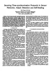
(22), τmax can be obtained from (21). Simulation results in Fig. 3 (see [25] and [26] for more detailed results) show that the Adaptive-Sync Protocol requires a far less number of timing messages than TPSN and RBS when there exist multiple number of beacon transmissions. Moreover, the gap between the average number of required timing messages between the Adaptive-Sync Protocol and TPSN and RBS significantly increases as N increases, and thus Adaptive-Sync is by far more energyefficient than TPSN and RBS for large N s. Moreover, the Adaptive Synch Protocol is applicable to various different types of sensor network applications. 22

Transmission Range = 25, Area = 100 × 100, Number of beacons (N) = 10 30000 25000 20000

Number of Timing Messages

15000

TPSN PBS (GPA) PBS (NPA) FTSP RBS

10000 8000 6000 4000

2000

1000 800 600 500 400 300 50

75

100

125 150 175 Number of Sensor Nodes (L)

200

225

250

Figure 3: Required number of message exchanges with respect to the number of sensor nodes.

4.3

Pairwise Broadcast Synchronization (PBS) Protocol

A major outcome of the work conducted in this project was the development of an energy-efficient clock synchronization scheme for wireless sensor networks (WSNs) based on a novel receiverreceiver synchronization approach. Within this synchronization approach, a subset of sensor nodes are synchronized by overhearing the timing message exchanges of a pair of sensor nodes. This represents a very practical and realistic scenario for wireless airborne networks because a group of sensor nodes can be synchronized without sending any extra messages. This novel synchronization protocol brings two main contributions. The first contribution is the development of a novel synchronization approach which can be partially or fully applied for implementation of new synchronization protocols and for improving the performance of existing time synchronization protocols. The second contribution consists in the design of a time synchronization scheme which significantly reduces the overall network-wide energy consumption without incurring any 23

Receiver-Only Synchronization

Region of Pairwise Sync. (Node P and Node A)

Sender-Receiver Synchronization

B

(2-Way Message Exchanges)

A

P Super Nodes

Figure 4: Receiver-only synchronization. loss of synchronization accuracy compared to other well-known schemes. Due to the power constraint, the communication range of a sensor is strictly limited to a (radio-geometrical) circle whose radius depends on the transmission power (see Fig. 4). In Fig. 4, every node within the checked area (e.g., Node B ) can receive messages from both Node P and Node A. Suppose that Node P is a parent (or reference) node, and Node P and Node A perform a pairwise synchronization using two-way timing message exchanges. Then, all the nodes in the checked region can receive a series of synchronization messages containing the information about the time stamps of the pairwise synchronization. Here, we assume perfect communications (no data loss and failure) at the physical layer. Using this information, Node B can be also synchronized to the parent node Node P by applying a similar method as in RBS and with no extra timing messages. Indeed, Node P and Node A can be regarded as super nodes since they provide synchronization beacons for all the nodes located in their vicinity. The work conducted in this project lead to the development of a new clock synchronization approach, named receiver-only synchronization (ROS). Similarly to Node B in Fig. 4, a group of

24

sensor nodes can be synchronized by only receiving timing messages of a pairwise synchronization based on ROS. The proposed PBS scheme efficiently combines both SRS and ROS approaches to achieve network-wide synchronization with a significantly reduced number of timing messages. Next we will describe and analyze the features of the proposed synchronization scheme in more detail.

4.3.1

Pairwise Sender-Receiver Synchronization

This subsection illustrates how a parent node Node P and Node A can be synchronized using (AP)

SRS. The clock model for the two-way message exchange is depicted in Fig. 5, where θof f set denotes the clock offset between Node A and Node P and timing messages are assumed to be exchanged multiple (N ) times [34], [8]. Hence, the number of observations (sets of time stamps) (A)

(A)

becomes N . Here, the time stamps transmitted during the ith message exchange T1,i and T4,i (P)

(P)

are measured by the local clock of Node A, and T2,i and T3,i are measured by the local clock of Node P, respectively. Node A transmits a synchronization packet to Node P, which contains the (A)

(P)

level and identifier (ID) of Node A and the value of time stamp T1,i . Node P receives it at T2,i (P)

and transmits an acknowledgement packet to Node A at T3,i . This packet contains the level and (A)

(P)

(P)

ID of Node P and the value of time stamps T1,i , T2,i , and T3,i . Then, Node A finally receives (A)

the packet at T4,i . Packet delays can be characterized into several distinct components: send, access, transmission, propagation, and receive time (see e.g., [34]). These delay components can be further divided into two parts: the fixed portions of delays in up- and down-link (d(AP) , d(PA) ) and the (AP)

variable portions of delays in up- and down-link (Xi

(PA)

, Xi

), respectively.

Thus far, several random delay models have been proposed. A single-server M/M/1 queue can fittingly represent the cumulative link delay for point-to-point connection, where the random 25

Node P

T3,1(P)

(P) T2,1

P

T2,i(P)

T2,(P)N

T3,(P) i

T3,(P) N

Clock Offset

(AP) θˆoffset

Node A

A (A) 4,1

(A) 1,1

T

T

T

(A) 4,N

T

T

T

T2,i(P)

(P) T2,1

Node B

(A) 1,N

(A) 4,i

(A) 1,i

(BP) θˆoffset

T2,(P)N

B (B) T2,1

T2,(B) N

T2,(B) i Di DN

Figure 5: Clock synchronization model of PBS. delays are modeled as exponential random variables [1]. The Gaussian delay model is appropriate if the delays are thought to be the addition of numerous independent random processes. In [7], the chi-squared test showed that the variable portion of delays can be modeled as Gaussian (AP)

distributed random variables with 99.8% confidence. In this letter, Xi

(PA)

and Xi

are assumed

to be normal distributed with mean µ and variance σ 2 /2. (P)

(A)

From Fig. 5, T2,i and T4,i can be expressed as (P)

= T1,i + θof f set + d(AP) + Xi

(A)

= T3,i + θof f set + d(PA) + Xi

T2,i T4,i (PA)

(A)

(AP)

(AP)

(P)

(PA)

(PA)

(AP)

(AP)

where θof f set = −θof f set , and d(AP) and Xi

,

,

denote the fixed and random portions of timing

delays in the message transmissions from Node A to Node P, respectively. In [27], the MLE of clock offset was found to be given by U −V (AP) (AP) , θˆof f set = arg max [ln L(θof f set )] = (AP) 2 θof f set (P)

(A)

(A)

(23) (P)

with the delays in up-link Ui , T2,i −T1,i and down-link Vi , T4,i −T3,i . From (23), Node A can be synchronized to the parent node Node P by simply taking the difference of the average delay 26

observations U = 1/N

PN

(P)

i=1

(A)

[T2,i − T1,i ] and V = 1/N

PN i=1

(A)

(P)

[T4,i − T3,i ]. Note that applying

a clock skew correction mechanism guarantees the long-term stability of synchronization, i.e., a decrease of the re-synchronization frequency. In [27], the joint maximum likelihood estimator of clock offset and skew for normal delays was derived. Although the effects of clock skew have not been considered herein, the clock skew estimators developed in [27] can be directly applied to the proposed PBS protocol with no modifications.

4.3.2

Receiver-Only Synchronization

In Fig. 4, consider an arbitrary node, say Node B, in the checked region. While Node P and Node A exchange time messages, Node B is capable of receiving packets from both nodes. Hence, (B)

Node B can observe a set of time readings ({T2,i }N i=1 ) at its local clock when it receives packets (P)

from Node A as depicted in Fig 5. Besides, the information about a set of time stamps {T2,i }N i=1 can also be obtained by receiving packets from Node P. Considering the effects of both clock (P)

offset and skew in this subsection, the time stamp at Node P in the ith uplink message T2,i is given by (P)

(A)

(AP)

(AP)

(A)

(A)

(AP)

T2,i = T1,i + θof f set + θskew · (T1,i − T1,1 ) + d(AP) + Xi

,

(24)

(AP)

where θskew stands for the relative clock skew between Node A and Node P. Likewise, the time (B)

stamp at Node B in the ith uplink message T2,i can be represented by (B)

(A)

(AB)

(AB)

(A)

(A)

(AB)

T2,i = T1,i + θof f set + θskew · (T1,i − T1,1 ) + d(AB) + Xi (AB)

,

(25)

(AB)

where θof f set and θskew stand for the relative clock offset and skew between Node A and Node B, (AB)

d(AB) and Xi

denote the fixed and random portions of timing delays in the message transmis(AB)

sion from Node A to Node B, respectively. Here, Xi RV with mean µ and variance σ 2 /2. 27

is assumed to be a normal distributed

Similar to [10], [13], and [36], the linear regression technique (line fitting) can be applied to synchronize Node B and compensate the effects of the relative clock skew between Node P and Node B. Subtracting (25) from (24) leads to (P)

(B)

(BP)

(BP)

(A)

(AP)

(A)

T2,i − T2,i = θof f set + θskew · (T1,i − T1,1 ) + d(AP) − d(AB) + Xi (AB)

Since d(AB) and d(AP) are fixed values and Xi

(AP)

and Xi (AP)

noise component can be defined by z[i] , µ0 + Xi (P)

.

(26)

are normal distributed RVs, the

(AB)

− Xi

(AB)

− Xi

, where µ0 , d(AP) − d(AB) and

(B)

z[i] ∼ N (µ0 , σ 2 ). Let define x[i] , T2,i − T2,i − µ0 and w[i] , z[i] − µ0 , then the set of observed data can be written in matrix notation as follows: x = Hθ + w, (BP)

(BP)

where x = [x[1] x[2] · · · x[N ]]T , w = [w[1] w[2] · · · w[N ]]T , θ = [θof f set θskew ]T , and 

T

1  1 H=  (A) (A) 0 T1,2 − T1,1

···

1

···

T1,N − T1,1

(A)

(A)

  . 

Note that the noise vector w is normally distributed w ∼ N (0, σ 2 I), and the matrix H represents the observation matrix of size N × 2. From [15, Theorem 3.2, p. 44], the least-squares estimator for the relative clock offset and skew is given by ˆ = (HT H)−1 HT x, θ

I(θ) =

HT H , σ2

where I(θ) is the Fisher information matrix. After some straightforward mathematical manipulations, the joint clock offset and skew estimator is given by    N N N N P P P P (BP) Di2 x[i] − Di [Di · x[i]]   θˆof f set  1  i=1 i=1 i=1 i=1 =  ·N ¸2    N N N N  P P P P P (BP) 2 N [D · x[i]] − D x[i] θˆskew Di N Di − i i i=1

i=1

i=1

28

i=1

i=1

   , 

(27)

(A)

(A)

where Di , T1,i − T1,1 . By inverting the Fisher information matrix I(θ), the Cramer-Rao lower bounds (CRBs) for the relative clock offset and skew take the expressions: σ2

(BP) var(θˆof f set )

N P

Di2 i=1 ≥ ·N ¸2 , N P P N Di2 − Di i=1

var(θˆskew ) ≥ (BP)

i=1

σ2N ·N ¸2 . N P P N Di2 − Di i=1

(28)

i=1

Consequently, using the results in (27), Node B can be synchronized to Node P. Likewise, all the other nodes in the checked region in Fig. 4 can be simultaneously synchronized to the parent node Node P without any additional timing message transmissions, thus saving a significant amount of energy. Fig. 6 shows the mean square error (MSE) performance of the proposed clock offset and skew estimators for ROS. It can be seen that both clock offset and skew estimators are efficient and their performance is well predicted by the CRBs. Besides, as we will see in the next section, ROS does not exhibit any loss of synchronization accuracy in clock offset estimation when compared to RBS.

4.3.3

Receiver-Receiver Synchronization

This section presents the RRS approach [7] and compares its performance with the proposed ROS approach. RRS is an approach to synchronize a set of children nodes that receive the beacon messages from the common sender, a reference or parent node. Consider a parent (reference) node P and arbitrary nodes A and B, located within the communication range of the parent node in Fig. 7. As depicted in Fig. 8, assume that both Node A and Node B receive the ith (A)

(B)

beacon from Node P at time instants T2,i and T2,i of their local clocks, respectively. Nodes A and B record the arrival time of the broadcast packet according to their own timescales and (PA)

then exchange their time-stamps. Suppose Xi

denotes the nondeterministic delay components

(random portion of delays) and d(PA) denotes the deterministic delay component (propagation

29

2

Mean Square Error

ROS Clock Offset and Skew Estimators (σ =1) Clock Offset Estimator CRLB

0

10

−1

10

5

10

15

20

25

30

35

40

45

50

−4

Mean Square Error

10

Clock Skew Estimator CRLB −6

10

−8

10

5

10

15

20 25 30 35 Number of Messages (N)

40

45

50

Figure 6: Performance of PBS clock offset and skew estimation. (A)

delay) from Node P to Node A, then T2,i can be written as (A)

(PA)

T2,i = T1,i + d(PA) + Xi

(PA)

(PA)

+ θof f set + θskew · (T1,i − T1,1 ), (PA)

(29)

(PA)

where T1,i is the transmission time at the reference node, θof f set and θskew are the clock offset and skew of Node A with respect to the reference node, respectively. Similarly, we can decompose the arrival time at Node B as (B)

(PB)

T2,i = T1,i + d(PB) + Xi (PB)

where d(PB) , Xi

(PB)

(PB)

(PB)

+ θof f set + θskew · (T1,i − T1,1 ),

(30)

(PB)

, θof f set , and θskew are the propagation (fixed) delay, the random portion of

delays, and the clock offset and skew of Node B, respectively. Subtracting (30) from (29), we obtain (A)

(B)

(BA)

(BA)

(PA)

T2,i − T2,i = θof f set + θskew · (T1,i − T1,1 ) + d(PA) − d(PB) + Xi (BA)

(PA)

(PB)

(BA)

(PA)

(PB)

(PB)

− Xi

,

(31)

where θof f set (= θof f set − θof f set ) and θskew (= θskew − θskew ) become the relative clock offset 30

Receiver-Receiver Synchronization

B P

A

Parent (Super) Node

Beacons

Figure 7: Receiver-receiver synchronization. and skew between Node A and Node B at the time they receive the ith broadcast packet from the reference node, respectively. Note that (31) assumes exactly the same form as (26). Hence, the same steps can be applied to derive the joint clock offset and skew estimator for ROS. (PA)

Likewise, define the noise component z[i] , µ0 + Xi (A)

(PB)

− Xi

, where µ0 , d(PA) − d(PB) and

(B)

z[i] ∼ N (µ0 , σ 2 ). Let also define x[i] , T2,i − T2,i − µ0 and w[i] , z[i] − µ0 . Using similar steps as in ROS, it is straightforward to show that the same form of the joint clock offset and skew estimator (27) can be also applied to RRS. Consequently, there is no difference between ROS and RRS with regard to the accuracy of synchronization since the effects of random delays are (BA)

the same. Assuming there is no clock skew (θskew = 0), the maximum likelihood estimator of (BA) the relative clock offset θˆof f set becomes N i 1 X h (A) (BA) (B) ˆ θof f set = T2,i − T2,i , N i=1

which is the equivalent to the estimator presented in [7].

31

(32)

4.3.4

Comparisons and Analysis

This section compares the proposed PBS with other well-known synchronization protocols, such as TPSN, RBS, and FTSP, with respect to the amount of energy consumption (number of required timing messages) and the synchronization accuracy. Lemma 1 Let NRBS be the number of required timing messages in RBS, then NRBS = N + L(L − 1)/2, where L is the number of overall sensor nodes in the network. The reference node must broadcast the beacon packet N times in RBS. Besides, every sensor node must send time readings upon receiving the broadcast beacons with all the other nodes in the network to compensate relative clock offsets among each other [7]. Thus, NRBS = N +L(L−1)/2, since the number of unique pairs in the network is L(L − 1)/2. Lemma 2 Let NTPSN be the required number of timing messages in TPSN, then NTPSN = 2N (L − 1). Since every node in the network is connected to its parent node except a reference node, there are L − 1 branches (edges) in a hierarchical tree. Besides, for TPSN, 2N timing messages are required in every pairwise synchronization. The number of required timing messages in TPSN is equal to the number of pairwise synchronizations times the number of required timing messages per pairwise synchronization, and therefore NTPSN = 2N (L − 1) [8]. Lemma 3 Let NFTSP be the number of required timing messages in FTSP, then NFTSP = N L. For FTSP, every sensor node must send its time readings upon receiving beacons (or broadcast beacons) to other nodes so that they can estimate the relative clock offsets among each other [22]. Therefore, the number of required timing messages in FTSP is equal to the number of sensor nodes times the number of beacons: NFTSP = N L. 32

Receiver-Receiver Synchronization (Node A and Node B)

Node P

P

Node A

A

T1,i

T1,1

T2,i(A)

(A) T2,1

(B) (A) T2,1 T2,1

Node B

B

T1, N

(B) T2,1

{T } {T } (B) i 2, j j =1

T2,i(B)

Clock Offset

T2,(A) N

{T } {T } (B) N 2, j j =1

(A ) i 2, j j =1

(A) N 2, j j =1

(AB) θˆoffset

(B) T2,N

Figure 8: Clock synchronization model of RBS. It is remarkable that the required number of timing messages for all the above mentioned protocols is proportional to the number of sensors in the network L or its square L2 . However, as discussed, PBS requires only 2N timing messages in every synchronization period, i.e., NPBS = 2N . Hence, NPBS dose not depend on the number of sensors in the network, which incurs an enormous amount of energy saving. Moreover, this gain proportionally increases with respect to the scale of the network. Consequently, the benefit of PBS over RBS, TPSN, and FTSP is clear and huge in terms of energy consumption with the cost of allocating 2 super nodes in the network. Note that RBS also requires a super node which broadcasts the reference beacons to all the other nodes in the network. In case that there are other sensor nodes which are located outside of the checked region in Fig. 4, likewise RBS, the network could be divided into a number of separated groups (clusters) and they could be synchronized by additional pairwise synchronizations among super nodes in different groups, i.e., global synchronization can be achieved by a sequence of pairwise synchronizations. Here, diverse grouping and pair selection algorithms can be considered according to the type of the network. For instance, assuming that the level hierarchy of the network is discovered by an appropriate searching algorithm (e.g., as in [8]), there exist groups of parents and 33

children nodes, where a group consists of a parent and its children nodes. Here, every parent node can investigate the connectivity among its children nodes and select the best sequence of synchronization pairs in order to minimize the required number of pairwise synchronizations, which maximizes the number of nodes performing ROS. Note that no network-wide heuristic connection search is required in this case because of its limited and known set of scanning nodes. The detailed description of these results for the proposed PBS scheme is reported in [25] and [26].

5

Conclusions

Time synchronization is a significant component in the deployment of wireless ad-hoc networks, and a number of fundamental operations, like data fusion, power management and transmission scheduling, require accurate time synchronization. Since the conventional NTP time synchronization protocol for the Internet can not be directly applied to wireless sensor networks and wireless airborne networks, a number of synchronization protocols have been developed in this project to meet the unique requirements of these applications. In this project, the basic features and theoretical backgrounds of the time synchronization problem in wireless sensor networks were first addressed and two general large scale network synchronization protocols were proposed. Besides, a survey of existing time synchronization protocols in the literature was provided including the most recent results. As the main contributions of this work, we can enumerate these major contributions. First, novel analytical tools and techniques to assess the performance of existing synchronization schemes were developed. Second, a family of novel joint clock offset and skew estimators based on the classical two-way message exchange model were also developed. Third, this work proposed two novel

34

energy-efficient time synchronization protocols: Adaptive-Sync Protocol and Pairwise Broadcast Synchronization (PBS) Protocol, which require a much lesser number of timing messages (energy consumption) than existing state-of-the-art synchronization protocols, and incur no loss in synchronization accuracy. A number of open research problems might be worth to investigate. Experimental performance evaluation and comparisons with other existing synchronization protocols represent a major open research work. More general random delay models might be needed for other network applications (such as presence of jamming, fading, node failures). Moreover, a variety of sophisticated statistical techniques, such as jackknife, bootstrap, and Gibbs sampling, could be applied to improve the performance of clock estimation. These remain open issues for another future research project.

35

References [1] H. S. Abdel-Ghaffar, “Analysis of synchronization algorithm with time-out control over networks with exponentially symmetric delays,”IEEE Trans. Commun., vol. 50, pp. 16521661, Oct 2002. [2] I. F. Akyildiz, W. Su, Y. Sankarasubramaniam, and E. Cayirci, “Wireless sensor networks: a survey,” Computer Networks vol. 38, no. 4, pp. 393-422, Mar. 2002. [3] I. F. Akyildiz, D. Pompili, T. Melodia, “Underwater Acoustic Sensor Networks: Research Challenges,” Elsevier’s Journal of Ad Hoc Networks, Vol. 3, Issue 3, pp. 257-279. [4] K. Arvind, “Probabilistic Clock Synchronization in Distributed Systems,” IEEE Transactions on Parallel and Distributed Systems, 5(5):474487, May 1994. [5] F. Cristian, “Probabilistic Clock Synchronization,” Distributed Computing, 3:146158, Springer-Verlag, 1989. [6] T. V. Dam, and K. Langendoen, “An adaptive energy-efficient MAC protocol for wireless sensor network,” Proceedings of the ACM Conference on Embedded Network Sensor Systems (Sensys), 2003. [7] J. Elson, L. Girod, and D. Estrin, “Fine-grained network time synchronization using reference broadcasts,” Proc. of the Fifth Symposium on Operating Systems Design and Implementation, (OSDI 2002), Dec. 2002. [8] S. Ganeriwal, R. Kumar, and M. B. Srivastava, “Timing-sync Protocol for Sensor Networks,” Proc. of the First ACM Conference on Embedded Networked Sensor Systems, (SenSys), Nov. 2003. 36

[9] S. Ganeriwal, D. Ganesan, H. Shim, V. Tsiatsis, and M. B. Srivastava, “Estimating Clock Uncertainty for Efficient Duty-Cycling in Sensor Networks,” ACM Sensys’05 Conference, pp. 130-141, Nov. 2005, San Diego, CA. [10] A. Giridhar and P. R. Kumar, “Distributed Clock Synchronization over Wireless Networks: Algorithms and Analysis,” in Proc. of the 45th IEEE Conference on Decision and Control, pp. 4915-4920, San Diego, Dec. 2006. [11] J. Heidemann, W. Ye, J. Wills, A. Syed, and Y. Li, “Research Challenges and Applications for Underwater Sensor Networking.” In Proceedings of the IEEE Wireless Communications and Networking Conference, (to appear) Las Vegas, Nevada, USA, April 2006. Available online: http://www.isi.edu/∼johnh/PAPERS/Heidemann06a.html. [12] Y. -W. Hong and A. Scaglione, “A scalable synchronization protocol for large scale sensor networks and its applications,” IEEE Journal on Selected Areas in Commun., vol. 23, no. 5, pp. 1085-1099, May 2005. [13] A. Hu and S. D. Servetto, “Asymptotically optimal time synchronization in dense sensor networks,” in Proc. of the 2nd ACM International Conference on Wireless Sensor Networks and Applications (WSNA), pp. 1-10, Sep. 2003. [14] D. R. Jeske, “On Maximum Likelihood Estimation of Clock Offset,” IEEE Transactions on Communications, Vol. 53, No. 1, pp. 53-54, Jan 2005. [15] S. Kay, Fundamentals of Statistical Signal Processing, Vol. I: Estimation Theory, vol. II: Detection Theory, Prentice-Hall, 1993.

37

[16] N. Khajehnouri and A. H. Sayed, “A distributed broadcasting time-synchronization scheme for wireless sensor networks,” in Proc. of ICASSP 2005, pp. 1053-1056, Philadelphia, March 2005. [17] J. Kong, J. Hong Cui, D. Wu, and M. Gerla, “Building underwater ad-hoc networks and sensor networks for large scale real-time aquatic applications.” In Proceedings of the IEEE MILCOM, Atlantic City, NJ, USA, Oct. 2005. [18] J. Lee, J. Kim and E. Serpedin, “Clock Offset Estimation in Wireless Sensor Networks Using Robust M-estimation”, WASA 2008 Conference, Dallas, TX, Oct. 2008 (submitted). [19] E. Lehman, Theory of Point Estimation, Wiley, 1986. [20] A. Leon-Garcia, Probability and Random Processes for Electrical Engineering, 2nd ed. Reading, MA: Addison-Wesley, 1993. [21] Q. Li and D. Rus, “Global clock synchronization in sensor networks,” IEEE INFOCOM, 2004. [22] M. Maroti, B. Kusy, G. Simon, A. Ledeczi, “The Flooding Time Synchronization Protocol”. In Proceedings of the 2nd International Conference on Embedded Networked Sensor Systems 2004, ACM Press, pp. 39-49. [23] D. L. Mills, “Internet Time Synchronization: The Network Time Protocol,” IEEE Trans. on Communications, vol. 39, no. 10, Oct. 1991, pp. 1481-1493. [24] S. B. Moon, P. Skelly, and D. Towsley, “Estimation and removal of clock skew from network delay measurements,” Proceedings of IEEE INFOCOM, 1, pp. 227-234, 1999.

38

[25] K. L. Noh, Y. C. Wu, K. Qaraqe, and B. Suter, “Extension of Pairwise Broadcast ClockSynchronization for Multi-Cluster Sensor Networks,” EURASIP Journal on Advances in Signal Processing, Special Issue on Applications of Signal Processing Techniques to Wireless Sensor Networks, January 2008 issue. [26] K. L. Noh, Y. C. Wu, K. Qaraqe, and E. Serpedin, “Time Synchronization for Wireless Sensor Networks,” book chapter in the Handbook: Adaptive Processing in Wireless Communications, CRC Press, (to be published in 2008). [27] K. Noh, Q. Chaudhari, E. Serpedin, and B. Suter, “Maximum Likelihood and Cramer-Rao Lower Bound for Clock Offset and Skew Estimation in Timing Synch Protocol for Sensor Networks,” IEEE Trans. on Communications, vol. 55, no. 4, pp. 766-777, Apr. 2007. [28] K. Romer, “Time Synchronization in Ad Hoc Networks,” Proceedings of ACM Symposium on Mobile Ad Hoc Networking and Computing, pp. 173182, Oct 2001. [29] B. M. Sadler, “Local and broadcast clock synchronization in a sensor node,” IEEE Signal Processing Letters, vol. 13, no. 1, pp. 9-12, Jan. 2006. [30] B. M. Sadler and A. Swami, “Synchronization in Sensor Networks: an Overview,” in Proc. of Military Communications Conference 2006, Washington D.C., Oct. 2006. [31] I. Sari, K. L. Noh, Q. Chaudhari, E. Serpedin, and B. Suter, “On the Joint Synchronization of Clock Offset and Skew in RBS-Protocol,” IEEE Trans. on Communications, vol. 56, no. 5, May 2008. [32] M. L. Sichitiu and C. Veerarittiphan, “Simple, accurate time synchronization for wireless sensor networks,” WCNC 2003.

39

[33] W. Su, and I. F. Akyildiz, “Time-diffusion synchronization protocol for wireless sensor networks,” IEEE/ACM Transactions on Networking, Volume 13, No. 2, pp. 384- 397, Apr 2005. [34] B. Sundararaman et al., “Clock synchronization for wireless sensor networks: a survey,” Ad-Hoc Networks, vol. 3, no. 3, pp. 281-323, Mar. 2005. [35] A. Syed and J. Heidemann, “Time Synchronization for High Latency Acoustic Networks,” Technical Report ISI-TR-2005-602, USC/Information Sciences Institute, April 2005. Available online: http://www.isi.edu/∼johnh/PAPERS/Heidemann06a.html. [36] Z. Tian, X. Luo, and G. B. Giannakis, “Cross-layer sensor network synchronization,” in Proc. of the 38th Asilomar Conference on Signals, Systems and Computers, vol. 1, pp. 1276-1280, Nov. 2004. [37] W. Ye, J. Heidemann, and D. Estrin, “An energy-efficient MAC protocol for wireless sensor networks,” Proceedings of the 21st International Conference of the IEEE Computer and Communications Societies (Infocom), 2002.

40

6

List of Symbols, Abbreviations, and Acronyms AO = Always On Adaptive Sync = Adaptive Synchronization CRLB = Cramer-Rao Lower Bound FTSP = Flooding Time Synchronization Protocol GPS = Global Positioning System ID = Identification iid = independent and identically distributed IP = Internet Protocol MAC = Medium Access Control ML = Maximum Likelihood MLE = Maximum Likelihood Estimator MSc = Master of Science MSE = Mean Square Error NTP = Network Time Protocol PBS = Pairwise Broadcast Synchronization PDF = Probability Density Function PhD = Doctor of Philosophy 41

RBS = Reference Broadcast Synchronization RF = Radio Frequency ROS = Receiver Only Synchronization RRS = Receiver Receiver Synchronization RV = Random Variable SI = Sensor Initiated SRS = Sender Receiver Synchronization TDMA = Time Division Multiple Access TDP = Time Diffusion Protocol TPSN = Time Protocol for Synchronization of Sensor Networks UAV = Unmanned Aerial Vehicles UDP = Universal Data Protocol WAN = Wireless Airborne Network WLAN = Wireless Local Area Network wrt = with respect to WSN = Wireless Sensor Network

42

7

List of Publications Resulted from this Project

[1] K. L. Noh, Q. Chaudhari, E. Serpedin, and B. Suter, “Novel Clock Phase Offset and Skew Estimation Using Two-Way Timing Message Exchanges for Wireless Sensor Networks,” IEEE Transactions on Communications, vol. 55, no. 4, April 2007, pp. 766-777. [2] I. Sari, K. L. Noh, Q. Chaudhari, E. Serpedin, and B. Suter, “On the Joint Synchronization of Clock Offset and Skew in RBS-Protocol,” IEEE Trans. On Communications, vol. 56, no. 5, May 2008. [3] Q. Chaudhari, E. Serpedin, and K. Qaraqe, “On Maximum Likelihood Estimation of Clock Offset and Skew in Wireless Sensor Networks with Exponential Delays,” IEEE Trans. On Signal Processing, . vol. 56, no. 4, April 2008. [4] K. L. Noh, Y. C. Wu, K. Qaraqe, and B. Suter, “Extension of Pairwise Broadcast ClockSynchronization for Multi-Cluster Sensor Networks,” EURASIP Journal on Advances in Signal Processing, Special Issue on Applications of Signal Processing Techniques to Wireless Sensor Networks, January 2008. [5] Q. Chaudhari and E. Serpedin, “A simple algorithm for clock synchronization in wireless sensor networks,” IEEE International Workshop “From Theory to Practice in Wireless Sensor Networks,” (T2PWSN 2007), Helsinki, Finland, June 2007. This workshop was part of IEEE International Symposium on a World of Wireless, Mobile and Multimedia Networks. [6] K. L. Noh, and E. Serpedin, “Pairwise broadcast synchronization in wireless sensor networks,” IEEE International Workshop “From Theory to Practice in Wireless Sensor Networks,” (T2PWSN 2007), Helsinki, Finland, June 2007. This workshop was part of IEEE International Symposium on a World of Wireless, Mobile and Multimedia Networks. [7] Q. Chaudhari, Y. Zhou, and E. Serpedin, “Efficient Clock Synchronization in Wireless Sensor

43

Networks,” Asilomar Conference 2007, Pacific Grove, CA, June 2007 (submitted for publication). [8] K. L. Noh, Y. C. Wu, K. Qaraqe, and E. Serpedin, “ Time Synchronization for Wireless Sensor Networks,” book chapter in the Handbook: Adaptive Processing in Wireless Communications, CRC Press, Submitted July 2007, (to be published in 2008). [9] Q. Chaudhari and E. Serpedin, “On maximum likelihood estimation of clock phase, skew and drift in networks with exponentially distributed delays,” EURASIP Journal on Advances in Signal Processing (accepted), Volume 2008, Article ID 219458, 6 pages [10] J. Lee, J.S. Kim, and E. Serpedin, “Robust bootstrap based clock offset estimators for wireless sensor networks,” WASA 2008 The International Conference on Wireless Algorithms, Systems and Applications (WASA’08), October 26-28, 2008, Dallas, (submitted). [11] Q. Chaudhari and E. Serpedin, “Clock Offset and Skew Estimation in Wireless Sensor Networks with Known Deterministic Delays and Exponential Nondeterministic Delays,” The Third International Conference on Digital Telecommunications (ICDT 2008), June 29 - July 5, 2008 (submitted). [12] Q. Chaudhari, E. Serpedin, and K. Qaraqe, “Statistical Signal Processing for Clock Synchronization in Wireless Sensor Networks,” WoSPA 2008 Conference [13] Q. Chaudhari and E. Serpedin, “Energy efficient synchronization algorithms for wireless sensor networks,” EUSIPCO 2008 Conference, (submitted). [14] Q. Chaudhari and E. Serpedin, “Clock Drift Estimation in Networks with Symmetric Exponential Link Delays,” submitted to 4th Advanced International Conference on Telecommunications (AICT), June 2008. [15] Kyoung-Lae Noh, “NEW ADVANCES IN DESIGNING ENERGY EFFICIENT TIME SYNCHRONIZATION SCHEMES FOR WIRELESS SENSOR NETWORKS,” PhD Thesis Dissertation, Texas A&M University, Dept. of Electrical and Computer Engineering, College Station, 44

TX, August 2007.

45