1038
IEEE TRANSACTIONS ON VERY LARGE SCALE INTEGRATION (VLSI) SYSTEMS, VOL. 12, NO. 10, OCTOBER 2004
Design of FPGA Interconnect for Multilevel Metallization André DeHon, Member, IEEE, and Raphael Rubin
Abstract—How does multilevel metallization impact the design of field-programmable gate arrays (FPGA) interconnect? The availability of a growing number of metal layers presents the opportunity to use wiring in the third dimension to reduce area and switch requirements. Unfortunately, traditional FPGA wiring schemes are not designed to exploit these additional metal layers. We introduce an alternate topology, based on Leighton’s mesh-of-trees (MoT), which carefully exploits hierarchy to allow additional metal layers to support arbitrary device scaling. When wiring layers grow sufficiently fast with aggregate network size ( ), our network requires only ( ) area; this is in stark contrast to traditional, Manhattan FPGA routing schemes where switching requirements alone grow superlinearly in . In practice, we show that, even for the admittedly small designs in the Toronto “FPGA Place and Route Challenge,” arity-4 MoT networks require 26% fewer switches than the standard, Manhattan FPGA routing scheme. Index Terms—Field programmable gate array (FPGA), hierarchical, interconnect, mesh-of-trees (MoT), multilevel metallization, Rent’s rule.
I. INTRODUCTION
V
LSI technology has advanced considerably since the first field-programmable gate arrays (FPGAs) [1]. Feature sizes have shrunk, die sizes and raw capacities have grown, and the number of metal layers available for interconnect has grown. The most advanced VLSI processes now sport 7–9 metal layers, and metal layers have grown roughly logarithmically in device capacity [2]. How should this shift in available resources affect the way we design FPGAs? One can view multilevel metallization, and particularly, the current rate of scaling, as an answer to the quandary that interconnect requirements for typical designs [Rent’s Rule [3], ; see (7)] grows faster than linearly with gate count [4], [5]. If we can accommodate the growing wire requirements in the third-dimension using multiple wire layers, then we may be able to maintain constant density for our devices. Alternately, if we cannot do this, the two-dimensional (2-D) density of our devices necessarily decreases as we go to larger device capacities. The existence of additional metal layers is not sufficient, by itself, to stave off this problem. We must further guarantee that we can contain the active silicon area to a bounded area per Manuscript received September 10, 2003; revised January 3, 2004. This research was funded in part by the Defense Advanced Research Projects Agency (DARPA) Moletronics Program under Grant ONR N00014-01-0651 and in part by the National Science Foundation CAREER program under Grant CCR-0133102. The authors are with the California Institute of Technology, Pasadena, CA 91125 USA (e-mail:
[email protected]). Digital Object Identifier 10.1109/TVLSI.2004.827562
device (e.g., an asymptotically constant number of switches per gate) and that we can topologically arrange to use the additional metallization. We show that the dominant, traditional, Manhattan style, interconnect scheme is not directly suited to exploiting multilevel metallization (Section II). Its superlinear switch requirements preclude it from taking full advantage of additional metal layers. The density of these architectures ultimately decreases with increasing gate count. We introduce an alternative topology, based on Leighton’s mesh-of-trees [6], [7] (MoT), which exploits hierarchy more strictly while retaining the 2-D interconnect style of the Manhattan interconnect (Section III). We show that this topology has an asymptotically constant number of switches per endpoint assuming no domain coloring limitations (Section IV-B). We further show that it can be arranged to fully exploit additional metal layers. As a result, given a sufficient interconnect layer growth rate, the gate density remains constant across increasing gate counts. In Section IV, we summarize a set of empirical experiments to compare the switch and wiring requirements of our MoT design to standard Manhattan routing topologies and characterize growth effects. In Section V, we explore several variations in the detail design of the MoT and identify versions which provide 26% fewer switches than the best known Manhattan designs. Table I summarizes the symbols used throughout the article. II. MANHATTAN INTERCONNECT A. Base Model Fig. 1 shows the standard model of a Manhattan (symmetric) [8], interconnect scheme. Each compute block (look-up table (LUT) or island of LUTs) is connected to the adjacent channels by a C-box. At each channel intersection is a switchbox (S-box). In the C-box, each compute block IO pin is connected to a fraction of the wires in a channel. At the S-box, each channel on each of the four sides of the S-box connects to one or more channels on the other sides of the S-box. Early experiments [8] studied the number of sides of the com, pute block on which each input or output of a gate appeared the fraction of wires in each channel each of these signals con, and the number of switches connected to each nected to . Regardless of the detail choices for wire entering an S-box these numbers, they have generally been considered constants, and the asymptotic characteristics are independent of the particular constants chosen. To keep this general, we will simply assume each side of the compute block has inputs or outputs to the channel. If
1063-8210/04$20.00 © 2004 IEEE
DEHON AND RUBIN: DESIGN OF FPGA INTERCONNECT FOR MULTILEVEL METALLIZATION
TABLE I SUMMARY OF SYMBOLS USED IN ARTICLE
1039
we are thinking about a single-output, -input LUT ( -LUT) . The number as our compute block, then of switches in a C-box is (1) where
is the width of the channel. Each S-box requires (2)
Each compute block comes with two C-boxes and one S-box (as shown highlighted in Fig. 1). So, the total number of switches per compute block is (3) Dropping the constants we get (4) That is, we see that the number of switches required per compute block is linear in , the channel width. We can get a loose bound on channel width simply by looking at the bisection width of the design. If a design has a minimum , then we have a lower bound on the channel bisection width width (5) That is, we must provide at least wires across the row (or column) channels which cross the middle of a chip with nodes. This allows us to solve for a lower bound on (6) Empirically, we find that the bisection width of a design can often be characterized by the Rent’s Rule relation [3] 1 (7) This now allows us to define a correspondence between
and
(8) This is the same correspondence which one gets by combining . This the results of Donath [10] and El Gamal [11] for means (9) All together, this says that as we build larger designs, if the interconnect richness is greater than , the switch requirement per compute block is growing for the Manhattan topology;
Fig. 1.
Manhattan interconnect model (W = 6, I = 2 shown).
1We might say the bisection width is determined by the IO out of each half, so BW = IO (N=2), rather than BW = IO (N ), but this would only make a constant factor difference and not change our asymptotic conclusions.
1040
IEEE TRANSACTIONS ON VERY LARGE SCALE INTEGRATION (VLSI) SYSTEMS, VOL. 12, NO. 10, OCTOBER 2004
where is the total number of hierarchical levels used. The total , is now number of wires in a channel, (12)
Fig. 2. Segmentation in Manhattan interconnect model (example shows L = 2).
this means the aggregate switching requirements grow superlinearly with the number of compute blocks supported. Regardless of the metallization offered, our designs will decrease in density with increasing gate count. B. Segmentation Modern designs, both in practice and in academic studies use segments which span more than one switchbox (see Fig. 2). For example, a recent result from Betz suggests that length 4–8 buffered segments require less area than alternatives [12]. The important thing to notice is that any fixed segmentation scheme only changes the constants and not the asymptotic growth factor in (9). In particular, using a single segmentation scheme will change (2) to of length (10) In practice the will be different between the segmented and nonsegmented cases, with the segmented cases requiring larger ’s, but the asymptotic lower bound relationship on derived above still holds. Similarly, a mixed segmentation scheme will also change the constants, but not the asymptotic requirements.
to the required bisecFor sufficiently large , we can raise in this hierarchical case does not, asymption width. Since totically, depend on , the number of switches converges to a constant. However, we should note this still does not change the asymptotic switch requirements, since the switch requirements depend on both the C-box switches and the S-box switches. As long as the C-box switches continue to connect to a constant fraction and not , the C-box contribution to the total number of of switches per compute block (1) continues to make the total and hence growing with . number of switches linear in From this we see clearly that it is the flat connection of block IO’s to the channel which ultimately impedes scalability. D. Switch Dominated Conventional experience implementing this style of interconnect has led some people to observe that switch requirements tend to be limiting rather than wire requirements (e.g., [12]). Asymptotically, we see that an -node FPGA will need (13) wires in the bisection and a number of wire layers, , With we will require at least (14) For fixed wire layers, this says wiring requirements grow slightly faster than switches (i.e., when , ). Asymptotically, this suggests that the number of layers must in order for the design to grow at least as fast as remain switch dominated. Since switches have a much larger constant contribution than wires, it is not surprising that designs require a large before these asymptotic effects become apparent.
C. Hierarchical A strictly hierarchical segmentation scheme might allow us to reduce the switchbox switches. Consider, that we have a base , and populate the channel with number of wire channels single length segments, length 2 segments, length 4 segments, and so forth. Using (10) with in for and summing across the geometric wire lengths, we see the total number of switches needed per switchbox is
III. MESH OF TREES The asymptotic analysis in Section II says that it is necessary to bound the compute block connections to a constant if we hope to contain the total switches per compute block to a constant independent of design size. Leighton’s MoT network [6], [7] is a topology which does just that. Simply containing the switches to a constant is necessary but not sufficient to exploit additional metal layers. Later in this section, we also show that the MoT topology can be wired within a constant layout area per compute block. A. Basic Arrangement
(11)
In the MoT arrangement, we build a tree along each row and column of the grid of compute elements (see Fig. 3). For now,
DEHON AND RUBIN: DESIGN OF FPGA INTERCONNECT FOR MULTILEVEL METALLIZATION
1041
as a single pass transistor and associated memory cell. Amortizing across the compute blocks which share a single tree, per compute block we need a total of (18) The horizontal channel holds such trees, as does the vertical channel. Thus, each compute block needs
(19) Using the linear corner turn population (16)
(20) Assuming we can hold bounded with increasing design size, this leaves us with a constant number of switches per compute block. B. Tree Growth
Fig. 3. Basic MoT topology.
we will assume the tree is binary (arity 2), but we can certainly vary the arity of the tree as one of the design parameters (Section V-A). The compute blocks connect only to the lowest level of the tree. A connection can then climb the tree in order to get to longer segments. We can place multiple such trees along each row or column to increase the routing capacity of the network. Each compute block is simply connected to the leaves of the set of horizontal and vertical trees which land at its site. We can parameterize the way the compute block connects to the leaf channels in a manner similar to the Manhattan C-box connections above. We will use the parameter to denote the number of trees which we use in each row and column. A MoT row or column is shown in Fig. 12(b). The C-box connections tree with at each “channel” in this topology are made only to the wires which exist at the leaf of the tree (15) In the simplest sense, we do not have switch boxes in this topology. At the leaf level, we allow connections between horizontal and vertical trees. Typically, we consider allowing each horizontal channel to connect to a single vertical channel in a domain style similar to that used in typical Manhattan switchboxes. This gives (16) It would also be possible to fully populate this corner turn, allowing any horizontal tree to connect to any vertical tree at points of leaf intersection without changing the asymptotic switch requirements (17) Within each row or column tree, we need a switch to connect each lower channel to its parent channel. This can be as simple
The strict binary tree we have shown correspondents to . To accommodate larger values, it is necessary to grow the number of parents in the tree. Returning to (8), we need the . We can arrange to per channel root bandwidth to be support a larger with the MoT by increasing the stage-to-stage growth rate. For example, if alternate tree levels double the number of (see Fig. 4). The parent segments, we can achieve number of tree levels is (21) where is the length of each row or column. The number of , composing the root level, , of each tree will thus channels, be
(22) The total bisection width at this level is the aggregate channel channels across the chip capacity across all (23) In this case that becomes (24) . That is, this growth is equivalent to providing Fig. 4 shows one-dimensional (1-D) slices of a (top) and a flat Manhattan topology (bottom). The MoT accommodates the bisection width of 4 using only a single base domain ), while the Manhattan topology requires at least one do( main for every wire in the bisection; this demonstrates how the MoT can often get away with a smaller than the Manhattan channel width ( ). The total channel wires for the MoT is 13 ). Asymptotically, the MoT will require six switches ( per endpoint for this arrangement, while the Manhattan design requires 8 to accommodate this channel width of 4. For larger
1042
IEEE TRANSACTIONS ON VERY LARGE SCALE INTEGRATION (VLSI) SYSTEMS, VOL. 12, NO. 10, OCTOBER 2004
Fig. 4. Row/column tree growth to achieve p = 0:75 and bisection width comparison with mesh.
we have no proof of the sufficiency of the population, so we employ empirical experiments, reported in Section IV, to assess the sufficiency of this population scheme.
TABLE II SWITCHES/NODE FOR p = 0:75 MoT
C. Basic Layout
spans, the effect increases. For a span of 32 nodes, the MoT can accommodate a bisection bandwidth of 8 while still using at most six switches per endpoint; the mesh with a bisection width of 8 will require 16 switches per endpoint. Note that even though we increased the rate of wire growth, the total number of switches per node remain asymptotically constant (see Table II) (25) Which makes (26) This property holds for any . That is, given sufficiently large , we can approximate any by programming the stage-to-stage growth rate, and the number of switches per compute block remains asymptotically constant. The particular constant grows with as this example suggests and is developed further in Section V-A. For arbitrary design bisection width, we that is equal to or greater than the design can pick a , and a network with constant switches per endpoint can provide that much bisection bandwidth. We are thus able to satisfy the lower bound relationship (8) introduced in Section II with constant switches per compute block. However, the lower bound relationship only guarantees that we have sufficient wires in the bisection, if we can use them. The population scheme will determine whether or not enough of the wires can be used to keep bound to a constant. At this point,
Constant switches per endpoint was necessary to show that we could layout the network in area linear in the number of compute blocks. However, it is not sufficient to show that we can use additional wire layers to achieve a compact layout. For unconstrained logic, it is not clear that more wire layers will always be usable. For example, [13] argues that wiring on an upper layer metal plane will occupy 12–15% of all the layers below it. Integrating this result across wire planes, this argues a useful limit of 6–7 wiring levels. The MoT wiring topology, however, is quite stylized with geometrically increasing wire lengths. Consequently, it does not exhibit the saturation effect which we would get with unconstrained netlists. Rather than consuming a constant fraction of lower layers, as [13] assumes, each additional metal layer in the MoT layout uses up a fraction of the layers below it that decreases geometrically with the layer height. In fact, we can show that a design which needs bisection bandwidth can be laid out with wiring layers. More specifically, only , we can use layers and maintain for any a constant channel width. : To build intuition, let us focus 1) Binary Tree . The key observation initially on the binary tree case is that we can layout each binary tree along its row (or column) wiring layers in a strip which is wide using and runs the length of the row . Fig. 5 shows how the row (column) tree is mapped into a wiring layers. It is important to no1-D layout with tice that each subtree layout leaves one free switch location for an upper level switch. When we combine two subtrees, we can place the switch connecting them in one of the two free slots, leaving a single slot free in the resulting subtree. In this manner, the recursive composition of subtrees can continue indefinitely; the geometrically increasing via spacing allows it to avoid ever running out of via area on the lower levels of metallization. As shown, each new tree level simply adds one additional wire run case requires above the existing wires. This
DEHON AND RUBIN: DESIGN OF FPGA INTERCONNECT FOR MULTILEVEL METALLIZATION
1043
Fig. 5. One-dimensional binary tree layout.
MoT tile with C = 4 and I = 2.
Fig. 6. Minimal MoT layout.
Fig. 7.
metal layers, which is asymptotically optimal to accommodate wires which each tree contributes to each row or the column. Note that if we make the width of the row as wide as a via and a wire, we can bring all the wires up to the appropriate metal layer without interfering with the row wire runs (See the “Top View” in Fig. 5). In practice, the width of a switch is likely to be several wire pitches wide; consequently, we can place several tree levels in a single metal layer and run them within the width of the switch row; this means that the number of wire layers we need for each where is row (or column) layout in practice is the ratio of the switch width to wire pitch (strictly speaking one less than that to accommodate the via row). For example, if the and the wire pitch is , we can put six switch width is wires within the width of the switch. If we use one track for vias, this means we can place five tree levels on each wire layer, so the number of layers needed to accommodate the row (column) tree is . The full MoT structures requires both row and column trees. We must space out the row and column switches to accommodate the cross switches. Further, we must assign separate wire layers for the rows and columns. Together, this means we will need layers for wiring. In practice, additional wiring layers will be needed for power, ground, and clock routing. Fig. 6 shows a minimal layout with a single tree in each row and column channel. In practice, we will typically use several in each row and column and require C-box trees
switches. Fig. 7 shows the base tile for a larger network configuration. : This same basic layout scheme 2) Fatter Trees . We will not always works for the case where have exactly half as many switches on each immediately succes, there are a number sive tree level. However, as long as of tree stages over which the number of switches will be half the number of switches in the preceding group of tree stages. By grouping the switches into these groups, we can use the same strategy shown for the binary tree case. Fig. 4 shows the switch arrangement for the aforementioned case. It should be clear from the layout tree diagrams that the switches can be shuffled to the base layer as in Fig. 5. Here, we will, asymptotically, end up with six switches between every pair of compute blocks (25). Up to a span of 16 endpoints, we need five switches (Table II). Beyond that, each pair of stages contributes half as many switches as the previous pair of stage, resulting in a total of one more switch per endpoint. As we compose each additional pair of stages we end up leaving half of the remaining slots in each span with space for switches from the next span. As shown in Fig. 4, we spread the uplinks across the entire width of the stage. This filling can continue indefinitely filling we have already seen. just as the Notice that the total number of metal layers is asymptoti, we must have cally optimal. That is, for wires in the top level of the channel to accommodate bisecwide, we must tion requirements. To make the channels layers to accommodate the bisection requireuse
1044
IEEE TRANSACTIONS ON VERY LARGE SCALE INTEGRATION (VLSI) SYSTEMS, VOL. 12, NO. 10, OCTOBER 2004
ments. The channel actually needs to accommodate all the wire levels of the MoT. Since there are geometrically fewer wires in , each lower level of each row or channel MoT tree when when we sum the total number of wires across all levels in each row or column tree, the total wire count is simply a constant factor times the number of wires in the top channel; this is developed further in Section V-A3. Consequently, the total number . of wire layers is D. Total Hierarchical Wires As we saw in Section II-C, when we have hierarchical wiring, , depends on the the total numbers of wires in the channel, level. For the MoT, the level is defined by the size of the device (21). The total number of wires in a channel is then (27) Equation (22) told us how to calculate for the case. Fig. 4 shows a MoT channel with , ; and . Later (30), we will see how to for any . calculate E. Switch Dominated The asymptotic reduction in switching requirements compared to the Manhattan topology makes wiring requirements more likely to be a limiting factor. At the same time, however, this topology allows us to maximally use additional metal layers. As a consequence, the MoT designs will always be switch area dominated when given sufficient layers of interconnect. F. Delay Note that switch delay is asymptotically logarithmic in the distance between the source and the destination. A route simply needs to climb the tree to the appropriate tree level to link to the destination row or column, then descend the tree. It is also worthwhile to note that the stub capacitance associated with each level of the tree is constant. That is, there are a constant number of switches (drivers or receivers) attached to each wire segment, regardless of its length. This is an important contrast with the flat, Manhattan connection scheme where the number of switches attached to a long wire is proportional to the length of the wire. An added benefit of the strict hierarchy is that it manages to minimize the switch capacitance associated with long wire runs. Buffered switches are needed to achieve minimum delay and to isolate each wire segment from the fanout that may occur on a multipoint net. G. Long Wire Runs Ultimately, we will need to buffer the long wire runs in order to achieve linear delay with interconnect length and minimize the delay traveling long distances. This will end up forcing us to insert buffers at fixed distances which can reduce the benefits of the convenient geometric switching property identified. Technological advances that provided linear delay with distance
without requiring repeaters (e.g., optical, superconducting wires) would obviate this problem. H. Relation to Tree-of-Meshes Agarwal [14], Lai [15], and Tsu [16] have previously described hierarchical FPGA interconnect architectures. DeHon showed that the butterfly fat-tree style interconnect of the hierarchical synchronous reconfigurable array (HSRA) could also be laid out in constant area given sufficient wire layers for the case [5]. These networks all build a single, unified hierarchy and are closely related to the tree-of-meshes topology [7]. In contrast, the MoT used here is directly a 2-D structure building hierarchical routing along each row and column. As such, the MoT can be viewed as a hybrid between the strict, single hierarchy of the tree-of-meshes and the nonhierarchical Manhattan array. A rigorous comparison of the tree-of-meshes and the MoT is addressed in [2121]. IV. EMPIRICAL EXPERIMENTS In Section III, we demonstrated the favorable asymptotic switching requirements for the MoT design assuming we can contain the number of required base channels, , to a suitably small constant. In this section we show empirically that the base channel requirements are uniformly small. Further, we show that even for the small sizes of conventional FPGA benchmarks, the MoT scheme already shows some practical advantages in reducing aggregate switch requirements. A. Base Comparison For a base level comparison, we use the benchmarks from Toronto’s “FPGA place and route challenge” [17] to compare the channel, domain, and switch requirements between the traditional Manhattan routing topology and our MoT topology. We architecture as the baseline used the mesh; this has single-length segments and a single LUT per Island. We substitute a universal switch [18] for the subset switch used in the vpr422 challenge because the routed mesh designs using universal switches uniformly require less switches than the subset-switch-based designs. Each of the 4 LUT inputs ap, and the pears on a single side of the logic block ; both are fully popuoutput appears on two sides lated [see Fig. 8(a)]. We use VPR 4.3 to produce the placed designs for both the Manhattan and MoT routing. We use the channel minimizing VPR 4.3 router to route the Manhattan designs. Since prior work suggested the superiority of longer segments [9], [12], we also routed a uniform, length-4 segment Manhattan case for comparison; all other parameters are identical to the base length-1 Manhattan case. For our overall comparison, we assembled a MoT design with [see Fig. 8(b)]. We developed our own, Pathfinder-based [19] router to route the MoT designs. To match the VPR-style results, we let the number of base channels, , float and report the minimum number of channels required to route the design for various values. Table III summarizes these basic results. For almost all deas to require signs, the MoT routes with sufficiently small fewer total switches than the Manhattan designs. Overall, the
DEHON AND RUBIN: DESIGN OF FPGA INTERCONNECT FOR MULTILEVEL METALLIZATION
Fig. 8.
Logic block IO structure (all shown
1045
W = 3).
TABLE III MANHATTAN VERSUS MESH-OF-TREES
potenused -LUT with a single output needs to have tially distinct signals enter one of the four channels which surrounds it. Further note that it shares each of those channels with another -LUT which has similar requirements. Consequently, the channel entrance lower bound is (28) For , . Finally, since the MoT design described here maintains the domain topology typical of Manhattan FPGA interconnect, it could have colorability limitations [20]. The routed results suggest that the colorability issues are not a major issue in practice as we are close to the channel entrance lower bound on all designs. V. MOT VARIATIONS There are many options for detailed construction of MoT networks which retain the good asymptotic characteristics derived in Sections II–IV while, perhaps, offering lower absolute switching and wiring requirements. In this section, we review a few options including arity, shortcuts, and staggering.
simple MoT requires 9% fewer switches than the mesh networks. than While the MoT designs require fewer base channels the Manhattan designs require wire channels , we noted in will be Section III-D that the total wires across all levels for instance, for the segment length larger. For for the . The 4 Manhattan design, while will have . As we will see in Section V, the MoT wiring can be reduced using higher arity trees. B. Small
’s
’s are uniformly small, many being as low as 3 for . We will see many more reduced to 3 or 4 with the variations in Section V. The required for the design is driven by three things: 1) bisection bandwidth; 2) number of distinct signals which must enter a channel; 3) domain coloring limitations. A sufficiently large value can generally accommodate bisection needs (see Fig. 4). For channel entrance, note that a fully The
A. Arity Arity refers to the branching factor as we go down the tree—the number of children segments associated with each parent segment in the tree. Fig. 9 shows arity-2 and arity-4 trees. Higher-arity makes the trees flatter. This will reduce the number of switches in a path, but will increase the capacitance associated with each segment along the path. Higher arity reduces the wires per domain, but can increase the number of domains needed to route a design. In particular, higher arity can force a number of short connections which would have been disjoint to now overlap [see Fig. 10(b)]. In the extreme, we completely flatten each channel into an tree. This would be equivalent to building a crossbar arityalong each column of tree. Such a crossbar would have channel , worse than the mesh, forcing a total number of width switches which grow as . So, clearly, we can make the arity too large to exploit the structure of designs. At the other extreme, arity-2 designs may have too many switches in the path and more intermediate levels than are useful. The challenge is
1046
IEEE TRANSACTIONS ON VERY LARGE SCALE INTEGRATION (VLSI) SYSTEMS, VOL. 12, NO. 10, OCTOBER 2004
Fig. 9. Single channel in 16 node row or column tree shown with various arities and rent growth rates.
Fig. 10.
MoT wiring versus arity.
to find the best balance point between these extremes which allows us to maximally exploit design structure. 1) Arity, Growth Rate, and Rent Exponent: For any arity, we can approximate any Rent Exponent growth rate by selecting the appropriate sequence of channel growths. Let , , at level . A MoT with levels has a total number of nodes,
(36) , we simply need , for all . For , For , we pick the sequence to correspond to the arity. For this means we make even ’s be two and odd ’s be one as previously noted in Section III-B [see Fig. 9(c)], so
(29) (37) The width of the top channel of a tree is Putting that in (36) (30) (38) The total bisection width,
, of a level MoT is For
, we make all
’s be 2 [see Fig. 9(d)]
(31) (39)
Using our Rent Relation (7), we have (32) (33) Here we see directly that the tree domain plays a similar role to the Rent constant multiplier, . To look at the growth effects, we drop these constants, understanding that we can use them to provide a constant shift on the bandwidth curves (34) (35)
Table IV summarizes the growth sequences used in this work. end2) Switches Per Domain: Amortized across the points sharing a single horizontal or vertical domain tree, each endpoint will have a number of tree switches (40) Equation (40) is the generalization of the arity-2, -specific switch counting illustrated in (18) and (25). Assuming the ’s are powers of two, Fig. 11 shows how the number of switches , higher arities have per domain varies with the arity. For fewer stages and hence less switches per endpoint, as should be , there are two competing effects. clear from Fig. 9. For Higher arities have fewer stages, but the higher arity results in flatting that forces each uplink to connect to a greater number
DEHON AND RUBIN: DESIGN OF FPGA INTERCONNECT FOR MULTILEVEL METALLIZATION
1047
TABLE IV GROWTH SEQUENCES USED TO ACHIEVE VARIOUS ARITY, RENT EXPONENT DESIGNS IN THIS ARTICLE
Fig. 11.
of parents. As shown, this results in a minimum number of . The switches per domain around an arity of 4 for odd powers of two end up being less efficient than the even , causing the powers in our discrete approximation to nonmonotonic growth in Fig. 11. Fig. 11 is not the full story as we must also understand how the number of tree domains changes (Section V-A.4) as we go to larger arities. 3) Wires Per Domain: In general, the number of wires per domain, , is the sum of the channels required at each level of , where is the tree level) each base tree (
Switches per endpoint per tree per domain.
TABLE V TOTAL SWITCHES VERSUS ARITY AND RENT EXPONENT (p)
(41)
For , it will always be the case that there are ’s series summation converges greater than one such that this , to a constant as approaches infinity. For arity 2 and the series converges to 3.5, while for arity 4 and , it converges to 2; Fig. 9 shows this effect graphically. For all ’s, higher arity implies higher growth rates and fewer terms in the sum resulting in fewer total wire channels. 4) Domains: An important question that the prior sections change with arity? raise is: how do the number of domains As Fig. 10 shows, sometimes a higher arity MoT will require no more base channels than the arity-2 MoT, resulting in a net decrease in total wires. Other times, the MoT may require a more base channels than the arity-2 MoT. factor of 5) Empirical Results: Tables V and VI summarize the resources required when each of the Toronto 20 benchmarks is required routed to minimize the number of tree domains to route the design. Note from Table VI that the ’s do not increase with arity near the worst-case ratios; in fact there is little growth for the cases shown. In Table V, we see an arity-4, requires only 1634 switches, about 14% fewer than the switches required by an arity-2 MoT. , (see SecThe total number of wires in the channel, tion III-D) is the product of the number of domains, , and the wires per domain, (41). Table VI further shows us that requires only of the arity-5, the wires required by the smallest arity-2 MoT. The total MoT are still larger than the mesh channel widths channel wires
. The worst-case for the , is 90, while the worst-case for the segment length 4 Mesh is 18. The 90 total MoT wires divide into nine wires used by each of ten domains. Conservatively assuming a minimum size switch and an wire pitch, we can route the nine wires in each domain over the width of a single switch in two wire pitches per layer (see metal layers since we get Figs. 5 and 7). Two wire layers for horizontal channel routing plus two layers for vertical channel routing mean we will need only four routing layers to layout this design so that it is the switch area which determines device density not the wiring. Consequently, the fact that the MoT reduces switches at the expense of wires compared to the mesh results in a net decrease in device area. B. Shortcuts and Staggering Perhaps the biggest concern about the MoT relative to a pure Manhattan design is the fact that some nodes which are physically close in the layout will not be logically close in the tree. This can, in the worst case, require a wire to travel through switches when two would suffice in the mesh or
1048
IEEE TRANSACTIONS ON VERY LARGE SCALE INTEGRATION (VLSI) SYSTEMS, VOL. 12, NO. 10, OCTOBER 2004
TABLE VI TREE DOMAINS (C ) AND WIRES PER CHANNEL (W ) VERSUS ARITY AND RENT EXPONENT (p)
total distance traversed is within a constant factor of the Manhattan Distance between the source and sink. Full shortcut population can double the tree switches per do. The general increase main required for an arity-2 MoT is (42)
Fig. 12.
Mitigating tree discontinuities with shortcuts and staggering.
MoT had this connection aligned differently with respect to the tree [see Fig. 12(a), (b), and (d)]. 1) Shortcuts: Shortcut connections which bridge these hierarchy gaps [see Fig. 12(c)] can guarantee that a signal never needs to be routed higher in the tree than . This also guarantees the
That is, we add one switch at each end of the arity group in addition to the switches already providing up tree connections.2 Table VII shows that while the shortcuts do reduce the number and the total wiring , their inclusion reof domains sults in a net increase in switch count. 2) Staggering: Most of the worst tree alignment effects can be reduced simply by staggering the domains relative to each other. This way, if there is a bad break on one tree, there will be a more favorable sibling relationship on another tree [see Fig. 12(d)]. In Section IV-B we established the minimum number of tree domains needed simply to exit all five IOs for , so there will always be multiple domains a 4-LUT is available for staggering. With larger clusters, the minimum domain size increase. Staggering the domains requires no additional switches and will often reduce the number of domains needed to route a design. Table VIII summarizes the mapped resource requirements when we stagger the tree domains in the channel. This shows an additional reduction of 14% in total wiring requirements and 5% in total switches . Overall, this brings the switch saving compared to the mesh to 26%. 2This can actually be (a + 1)=a as we only need one switch to enable or disable the shortcut so we only need to charge half a switch to each of the two segments being connected. However, as we get higher in the tree, having a single switch could result in a long wire stub. In practice, we might use one switch at the lower levels and two at the upper levels.
DEHON AND RUBIN: DESIGN OF FPGA INTERCONNECT FOR MULTILEVEL METALLIZATION
TABLE VII PROPERTY SUMMARY VERSUS ARITY FOR p = 0:67 WITH SHORTCUTS
1049
implications. A careful accounting and comparison of delay and energy are important pieces of future work which will be necessary to establish the practical viability of this scheme. We have explored many of the parameters associated with designing MoT networks but additional design parameters deserve study including Island-style clustering, flattening, corner turns, and depopulated shortcuts. We expect larger benchmarks will better demonstrate the scalability of this architecture.
REFERENCES
TABLE VIII PROPERTY SUMMARY VERSUS ARITY AND RENT EXPONENT (p) WITH DOMAIN STAGGERING
VI. SUMMARY AND FUTURE WORK
Using the MoT topology, we can achieve better scalability than a flat, Manhattan topology. Assuming the number of base channels, , remains constant for increasing design size, the total number of switches per LUT in our MoT converges to a independent of design size; this should be conconstant trasted with the switches per LUT required for a flat, Manhattan topology. Given sufficient wiring layers, the MoT network layout can maintain a constant area per logic block as the design scales up. Asymptotically, the number of switches in . Our iniany path in the MoT needs to only grow as tial empirical experiments verify small values that show no signs of growing with design size and total switch requirements that are 26% smaller than those of conventional mesh designs. In the process we show that arity-4 trees require the least absolute switches with less than 70% of the wiring requirements of arity-2 trees. In this paper, we have focused on the resource requirements for the MoT, but have not treated the absolute delay or energy
[1] W. S. Carter, K. Duong, R. H. Freeman, H.-C Hsieh, J. Y. Ja, J. E. Mahoney, L. T. Ngo, and S. L. Sze, “A user programmable reconfigurable logic array,” in IEEE 1986 Custom Integrated Circuits Conf., May 1986, pp. 233–235. [2] M. Bohr, “Interconnect scaling—The real limiter to high performance ulsi,” in Int. Electron Devices Meeting 1995 Tech. Dig., Dec. 1995, pp. 241–244. [3] B. S. Landman and R. L. Russo, “On pin versus block relationship for partitions of logic circuits,” IEEE Trans. Computers, vol. 20, pp. 1469–1479, 1971. [4] A. DeHon, “Rent’s rule based switching requirements,” in Proc. SystemLevel Interconnect Prediction Workshop, Mar. 2001, pp. 197–204. [5] , “Compact, multilayer layout for butterfly fat-tree,” in Proc. 12th ACM Symp. Parallel Algorithms Architectures , July 2000, pp. 206–215. [6] F. T. Leighton, Introduction to Parallel Algorithms and Architectures: Arrays, Trees, Hypercubes: Morgan Kaufmann , 1992. [7] , “New lower bound techniques for VLSI,” in Proc. Annual Symp. Foundations of Computer Science, 1981. [8] S. D. Brown, R. J. Francis, J. Rose, and Z. G. Vranesic, Field-Programmable Gate Arrays. Norwell, MA: Kluwer , 1992. [9] V. Betz, J. Rose, and A. Marquardt, Architecture and CAD for DeepSubmicron FPGAs. Norwell, MA: Kluwer, 1999. [10] W. E. Donath, “Placement and average interconnection lengths of computer logic,” IEEE Trans. Circuits Syst., vol. 26, pp. 272–277, Apr. 1979. [11] A. E. Gamal, “Two-dimensional stochastic model for interconnections in master slice integrated circuits,” IEEE Trans. Circuits Syst., vol. 28, pp. 127–138, Feb. 1981. [12] V. Betz and J. Rose, “FPGA routing architecture: Segmentation and buffering to optimize speed and density,” in Proc. Int. Symp.Field-Programmable Gate Arrays, Feb. 1999, pp. 59–68. [13] G. A. Sai-Halasz, “Performance trends in high-end processors,” Proc. IEEE, vol. 83, pp. 20–36, Jan. 1995. [14] A. A. Agarwal and D. Lewis, “Routing architectures for hierarchical field programmable gate arrays,” in Proc. 1994 IEEE Int. Conf. Computer Design, Oct. 1994, pp. 475–478. [15] Y.-T. Lai and P.-T. Wang, “Hierarchical interconnection structures for field programmable gate arrays,” IEEE Trans. VLSI Syst., vol. 5, pp. 186–196, June 1997. [16] W. Tsu, K. Macy, A. Joshi, R. Huang, N. Walker, T. Tung, O. Rowhani, V. George, J. Wawrzynek, and A. DeHon, “HSRA: High-speed, hierarchical synchronous reconfigurable array,” in Proc. Int. Symp. Field-Programmable Gate Arrays, Feb. 1999, pp. 125–134. [17] V. Betz and J. Rose. (1999) FPGA Place-and-Route Challenge. [Online]. Available: http://www.eecg.toronto.edu/~vaughn/challenge/challenge.html [18] Y.-W. Chang, D. F. Wong, and C. K. Wong, “Universal switch-module design for symmetric-array-based FPGA’s,” in Proc. Int. Symp. FieldProgrammable Gate Arrays, Feb. 1996, pp. 80–86. [19] L. McMurchie and C. Ebling, “Pathfinder: A negotiation-based performance-driven router for FPGAs,” in Proceedings of the International Symposium on Field-Programmable Gate Arrays, Feb. 1995, pp. 111–117. [20] Y.-L. Wu, S. Tsukiyama, and M. Marek-Sadowska, “Graph based analysis of 2-d FPGA routing,” IEEE Trans. Computer-Aided Design, vol. 15, pp. 33–44, Jan. 1996. [21] A. DeHon, “Unifying mesh- and tree-based programmable interconnect,” IEEE Trans. TVLSI Syst., vol. 12, pp. 1051–1065, Oct. 2004.
1050
IEEE TRANSACTIONS ON VERY LARGE SCALE INTEGRATION (VLSI) SYSTEMS, VOL. 12, NO. 10, OCTOBER 2004
André DeHon (S’92–M’96) received the S.B., S.M., and Ph.D. degrees in electrical engineering and computer science from the Massachusetts Institute of Technology, Cambridge, in 1990, 1993, and 1996, respectively. From 1996 to 1999, he was Co-Head of the BRASS Group, Computer Science Department, University of California, Berkeley. Since 1999, he has been an Assistant Professor of Computer Science at the California Institute of Technology. He is broadly interested in how we physically implement computations from substrates, including VLSI and molecular electronics, up through architecture, CAD, and programming models. He places special emphasis on spatial programmable architectures (e.g., field-programmable gate-arrays) and interconnect design and optimization.
Raphael Rubin received the B.S. degree in engineering and applied sciences from the California Institute of Technology, Pasadena, CA, in 2001. Since 2001, he has worked as a Research Associate for the Implementation of Computation Group in the Computer Science Department, California Institute of Technology. His research interests include programmable interconnect and design automation.