Design of Optimally Reinforced RC Beam, Column, and Wall Sections Downloaded from ascelibrary.org by UGR/E.U ARQUITECTURA TECNICA on 05/29/14. Copyright ASCE. For personal use only; all rights reserved.
Mark Aschheim1; Enrique Hernández-Montes2; and Luisa María Gil-Martín3 Abstract: A conjugate gradient search method is coupled with a general model for the ultimate strength of a rectangular reinforced concrete 共RC兲 cross section. Reinforcement required to provide reliable resistance identically equal to required strengths 共due to factored load effects兲 is determined. The total reinforcement is determined optimally, either to obtain a global minimum or to obtain a minimum subject to various constraints, such as the use of equal reinforcement on opposite faces or the use of equal reinforcement on all faces. The model is useful for the design of beam, column, and wall sections that are subjected to uniaxial or biaxial bending. Solutions are obtained directly, and make use of computing power contained within spreadsheet programs that are widely available. Avoiding the somewhat tedious hand calculations and approximations required in conventional iterative design approaches avoids errors and potentially unsafe designs, while the use of optimum reinforcement quantities advances the aim of improving the sustainability of RC construction. DOI: 10.1061/共ASCE兲0733-9445共2008兲134:2共231兲 CE Database subject headings: Concrete columns; Concrete beams; Walls; Bending.
Introduction While the same fundamental assumptions are used for the flexural design of beam, column, and wall sections in model building codes such as ACI-318 共ACI 2005兲, current approaches for the design of these sections differ significantly. Algebraic expressions for ultimate strength typically are used to determine the amount of primary longitudinal reinforcement in beams. Beam reinforcement is placed at its most effective location in the section. For the design of columns, however, the longitudinal reinforcement typically is assumed to be distributed in a predetermined pattern, and previously prepared uniaxial P-M interaction curves often are used for determining the amount of longitudinal reinforcement. Where biaxial bending occurs, approximate expressions introduced by Bresler 共1960兲 or Gouwens 共1975兲 often are used in conjunction with uniaxial P-M interaction curves; the resulting design may be validated with a rigorous sectional analysis. For walls, distributed web reinforcement is considered, possibly supplemented by concentrated longitudinal reinforcement at the ends of the walls; this reinforcement is often determined on the basis of preliminary hand calculations and verified using a more rigorous sectional analysis. While beams are designed optimally on the basis of algebraic solutions, column and wall design often requires a number of iterations in conjunction with approximate 1
Associate Professor, Santa Clara Univ., 500 El Camino Real, Santa Clara, CA 95053 共corresponding author兲. E-mail:
[email protected] 2 Associate Professor, Campus de Fuentenueva, Univ. of Granada, 18072 Granada, Spain. E-mail:
[email protected] 3 Associate Professor, Campus de Fuentenueva, Univ. of Granada, 18072 Granada, Spain. E-mail:
[email protected] Note. Associate Editor: M. Asghar Bhatti. Discussion open until July 1, 2008. Separate discussions must be submitted for individual papers. To extend the closing date by one month, a written request must be filed with the ASCE Managing Editor. The manuscript for this paper was submitted for review and possible publication on August 21, 2006; approved on May 30, 2007. This paper is part of the Journal of Structural Engineering, Vol. 134, No. 2, February 1, 2008. ©ASCE, ISSN 0733-9445/2008/ 2-231–239/$25.00.
formula and the placement of some reinforcement where it has reduced effectiveness. Approximations for biaxial bending have been the source of controversy. Hoffman et al. 共1998兲 illustrate that Bressler’s reciprocal load relationship is unconservative, and recommend it not be used “except for columns with large axial loads such that little or no tensile stress exists at any point of the cross section” 共p. 292兲. Lepage-Rodriguez 共1991兲 compared several approximations for biaxial bending with the results of sectional analyses. Furlong et al. 共2004兲 compared biaxial strength estimates with the results of experimental and computational studies. They found that the elliptical load contour represented experimental strengths more accurately than the reciprocal load method 共which generally was conservative兲; however, scatter in the experimental data relative to the estimated strengths led the authors to recommend modifications to reduce the likelihood that this method would be unconservative. A rigorous sectional analysis was shown to represent experimental strengths well, with the ratio of measured strength to estimated strength having mean equal to 1.030 and coefficient of variation of 9.3%. Ubiquitous desktop computing power now makes the generation 共analysis兲 of the full three-dimensional 共3D兲 interaction curve 共P-M x-M y兲 straightforward with software such as PCAColumn 共PCA 2005兲, CSiCol 共2006兲, and BIAX-2 共Wallace 1992兲, by repeated applications of the fundamental sectional analysis assumptions for different locations and inclinations of the neutral axis. Such software may be used to validate a design that was originally developed on the basis of approximate formulae or interaction charts 共as suggested by MacGregor and Wight 2005兲, and may be used directly for design by repeated analysis of trial sections until an efficient, constructible, and safe, design is identified. Such software also can be used to design walls by a similar sequence of iteration. With the exception of beam design, these approaches generally emphasize analysis of a section with known reinforcement rather than the direct solution of the reinforcement required to provide a section with adequate strength. In recent work, the writers have reformulated the sectional design problem to determine the re-
JOURNAL OF STRUCTURAL ENGINEERING © ASCE / FEBRUARY 2008 / 231
J. Struct. Eng. 2008.134:231-239.
Downloaded from ascelibrary.org by UGR/E.U ARQUITECTURA TECNICA on 05/29/14. Copyright ASCE. For personal use only; all rights reserved.
quired reinforcement directly, for a given neutral axis location and required strength. This formulation allows a neutral axis location to be identified that results in a reduction in total reinforcement relative to that obtained when a predetermined pattern of reinforcement is used. This approach was described for uniaxial bending by Hernández-Montes et al. 共2005兲, and led to an evaluation of the effect of optimal reinforcement on curvature ductility 共Hernández-Montes et al. 2004兲, the characterization of optimal solutions over the P-M space 共Aschheim et al. 2007兲, and the formulation of a theorem governing the optimal design of sections for uniaxial bending 共Hernández Montes et al. 2006b兲. More recently, the approach was extended to biaxial bending using the spacing of reinforcement on the side faces relative to that on the top and bottom faces as an explicit variable 共Hernández Montes et al. 2006a兲. The present paper uses a nonlinear conjugate gradient search technique to obtain a general solution for the optimal reinforcement of rectangular reinforced concrete sections for a general P-M x-M y load combination. The approach may be used to obtain solutions for the design of cross sections for uniaxial or biaxial bending, using conventional 共symmetric兲 distributions of reinforcement, or using optimal distributions, which generally lack symmetry. Examples illustrate the application of this approach for beam, column, and wall cross sections. The solution technique greatly simplifies design, since a single model is used to obtain conventional or optimal solutions for beams, columns, and walls in just a few keystrokes, eliminating the need for column design charts, biaxial bending approximations, and tedious hand calculations and iterations in some cases. Because the process is automated, the opportunity for mistakes to be made using a combination of hand calculations, tables, and approximate formulae in multiple design iterations is greatly reduced. Columns, walls, and other members subjected to symmetric loading generally will be reinforced with a symmetric distribution of reinforcement. Some beam-type members may be subjected to axial loads in conjunction with bending, while other column-type members may be subjected to asymmetric loading, such as edge and corner columns of buildings, the bridge columns used in “C-bent” configurations, and the walls of box culverts. For such members, optimal reinforcement can reduce the amount of longitudinal reinforcement by up to 50% 共Hernández Montes et al. 2005兲. The savings in reinforcement has implications for reducing cost and also provides a much-needed innovation to improve the sustainability of reinforced concrete construction.
Problem Formulation and Solution A reinforced concrete section is to be designed to simultaneously carry a factored axial force, Pu and factored moments, M ux and M uy, about the x and y axes of the section, respectively. The general requirement that the factored load effects must not exceed the nominal resistances can be expressed as Pu 艋 Pn, M ux 艋 M nx, and M uy 艋 M ny, where ⫽strength reduction factor. The design loading 共Pu, M ux, M uy兲 can be expressed equivalently as an axial load located at eccentricities ex and ey from the origin along the x and y axes, respectively, where ex = M uy / Pu and ey = M ux / Pu, and the origin is located at the geometric centroid of the gross section. The case with positive eccentricities is illustrated in Fig. 1, superposed over the idealized reinforced concrete section. Although discrete reinforcing bars will be used in an actual
Fig. 1. Problem formulation
design, for the purposes of optimal proportioning, the reinforcement along a face is considered to be distributed uniformly, or smeared, into a single, continuous plate that is inset from the edge of the section. The distance from the edge of the section to the centroid of the reinforcement plate is assumed equal to d⬘ along the edge of length h, and equal to b⬘ along the edge of length b, as shown in Fig. 1. The amount of reinforcement along each face may differ, resulting in the quantities As,t, As,b, As,l, and As,r distributed along the top, bottom, left, and right faces of the section, respectively. Standard section analysis assumptions that are recognized by ACI 318 共ACI 2005兲 are used. The Bernouilli hypothesis 共plane sections remain plane兲 is assumed, with ultimate strength defined by the attainment of a peak usable compressive strain of 0.003 at the extreme fiber of the concrete section. For the positive values of eccentricity shown in Fig. 1, the neutral axis is located at a depth c from the top right corner of the section, and is inclined at an angle . In general, the inclination of the neutral axis differs from the inclination of the vector combination of the applied moments. The strength reduction factor, , is a function of the net tensile strain, t, which is defined as the tensile strain at the extreme tension steel. For tied columns, varies from 0.65 for t 艋 0.002 to 0.90 for t 艌 0.005, and varies linearly between these strain limits. Thus, can be evaluated in any analysis in which c and are known 共along with the dimensional data needed to define the section兲. ACI 318 allows use of a stress block 共Whitney and Cohen 1956兲 to represent the stress carried by the concrete in compression. A compressive stress of 0.85f ⬘c is assumed to be carried by the concrete over a depth 1c, measured from the top right corner of the section 共Fig. 1兲. The factor 1 assumes a value of 0.85 for specified strength f ⬘c less than 27.6 MPa 共4,000 psi兲, 0.65 for f ⬘c 艌 55.2 MPa 共8,000 psi兲, and varies linearly between these values for intermediate strengths. The portion of the section sustaining this stress is shown with shading in Fig. 1. For purposes of analysis, this region can be divided into discrete regions, each with their own resultant 共given by the product of stress and area兲. The resultants may be evaluated after determining which case among those illustrated in Fig. 2 is applicable. The case 1c ⬎ zb is not illustrated, but corresponds to the compression block extending over the entire cross section. Following ACI 318, the concrete is assumed to carry no tensile stress.
232 / JOURNAL OF STRUCTURAL ENGINEERING © ASCE / FEBRUARY 2008
J. Struct. Eng. 2008.134:231-239.
Downloaded from ascelibrary.org by UGR/E.U ARQUITECTURA TECNICA on 05/29/14. Copyright ASCE. For personal use only; all rights reserved.
Fig. 2. Cases for determination of concrete contribution
According to ACI 318, the steel reinforcement is considered to have elastoplastic behavior, with yield strength equal to the specified yield strength, f y, and modulus of elasticity Es. In general, the strain gradient over the height of the section may cause the steel along any one face to have portions that are elastic and portions that are yielding in tension or compression. The strain diagram applicable to the analysis is associated with reinforcement stresses as shown generically in Fig. 1. For purposes of analysis, each reinforcement “plate” is considered as follows: 共1兲 the strains at each end of the reinforcement “plate” are determined; 共2兲 based on these strains, the portions of the reinforcement plate that are yielding in tension, that are elastic, and that are yielding in compression are identified; and 共3兲 the magnitude and location of the resultants associated with each of these portions are then determined. The resultants, of course, are given as the integral of the stress over the respective length of plate, and act at the centroid of the stress distribution. Finally, to avoid double counting the contributions of the reinforcement and concrete in compression, the length of reinforcement plate that overlaps the concrete compression zone is determined, and the resultant force 共associated with a stress of 0.85f ⬘c 兲 is considered as a tensile contribution to equilibrium. This approach is used for the distributed reinforcement 共plate兲 along each face. Following this approach, the internal stress resultants and their locations are determined, for any neutral axis depth, c, and inclination . The external loads 共Pu / , M ux / , M uy / 兲 that equilibrate these internal stress resultants may be determined by a straightforward application of equilibrium. A conventional analysis would evaluate strength given values of As,t, As,b, As,l, and As,r. In the present case, the amounts of reinforcement required to confer adequate resistance to the section are determined, as follows.
In general, we seek non-negative values of steel areas 共As,t 艌 0 , As,b 艌 0 , As,l 艌 0, and As,r 艌 0兲 such that equilibrium is satisfied 共⌺F = 0, ⌺M x = 0, ⌺M y = 0兲 at the section level. Because equilibrium provides three constraints, while there are six unknowns 共As,t , As,b , As,l , As,r, c, and 兲 an infinite number of satisfactory combinations of reinforcement steel areas may be identified. Consequently, the total reinforcement area 共As,t + As,b + As,l + As,r兲 may be minimized subject to the preceding constraints. This is a nonlinear optimization problem. Solutions may be found efficiently using nonlinear conjugate gradient search methods. While a rigorous approach to the solution may be implemented 共e.g., Nocedal and Wright 1999兲 it is far simpler in practice to formulate the problem using a spreadsheet program such as Excel 共2003兲, where optimal solutions may be obtained in just a few keystrokes using the Solver add-in. Using this representation, optimization becomes a powerful tool that can be used to support design decionmaking, since the engineer can craft a solution that addresses considerations that lay both within and beyond the formal optimization problem. To guide the solution, additional constraints on 共0 艋 艋 / 2兲 and c 共0 艋 c 艋 10h兲 may be useful. As stated, the problem in six unknowns and three equations of equilibrium has three degrees of freedom. Additional constraints can be imposed at the behest of the designer. For example, a designer may set steel areas along one or more sides equal to zero, or equal to one another. If three such constraints are imposed 共e.g., As,t = As,b = As,l = As,r兲, then the problem has a single solution, which corresponds to that obtained with conventional P-M interaction charts in the case of uniaxial loading. Therefore, the formulation may be considered to be general, since it allows for optimization while including as a subset the class of widely accepted, conventional solutions.
Admissible Solutions To illustrate the application of the method and range of potential solutions, optimal solutions were obtained as a function of c and for an example column section. The example section is based on one whose strength was evaluated by MacGregor and Wight 共2005, p. 525兲 for a particular depth and inclination of neutral axis. Minimum reinforcement required to provide the section with the same nominal strength 共Pn = 383 k, M nx = 1995 k in., and M ny = 989 k in.兲 was determined for different values of c and . Minimum reinforcement solutions are shown for each value of c and where such solutions could be obtained, along with contours. The global minimum is given by g = 2.22%, and occurs for c / h = 0.750 and = 38.8° 关this section is illustrated in Fig. 8共e兲兴. Small sketches superimposed on Fig. 3 indicate the distribution of reinforcement over the section for four combinations of c / h and . Clearly, very different patterns of reinforcement may be used to provide a section with a desired nominal strength. For comparison, the symmetric reinforcement solution 共equal reinforcement on all faces兲 requires g = 2.72%, and is obtained for c / h = 0.784 and = 30.0°. Constraints may be imposed on the reinforcement areas to obtain solutions mimicking conventional column reinforcement distributions. Where equal reinforcement areas are desired on opposite faces 共As,t = As,b and As,l = As,r兲, the variables As,b and As,r may be set equal to the values used on the opposite faces, and values of As,t and As,l are sought that minimize the objective function 共As,t + As,b + As,l + As,r, for example兲. Similarly, if equal reinforcement areas on all faces are desired, three reinforcement
JOURNAL OF STRUCTURAL ENGINEERING © ASCE / FEBRUARY 2008 / 233
J. Struct. Eng. 2008.134:231-239.
Downloaded from ascelibrary.org by UGR/E.U ARQUITECTURA TECNICA on 05/29/14. Copyright ASCE. For personal use only; all rights reserved.
Fig. 3. Contours of total reinforcement 共expressed as percent of gross section area兲 required to provide Pn = 383 k, M nx = 1995 k in., and M ny = 989 k in. as function of c/h and
areas may be set equal to a fourth, and values of the fourth are sought that minimize the objective function. Thus, conventionally reinforced concrete columns may be designed for biaxial loading with only a few keystrokes. This is easier and more reliable than the use of uniaxial P-M interaction charts in combination with approximate expressions for biaxial bending, or the use of specialized commercial software to repeatedly check and refine a design based on the computed 共Pn , M nx , M ny兲 interaction surface. For beam design it is not necessary to constrain the top or side reinforcement areas to zero, as the optimal solution will naturally determine the required amount of bottom reinforcement. Where relatively large moments exist, the reduction in as a function of t 共prescribed by ACI 318兲 causes the optimal solution to provide sufficient top 共compression兲 reinforcement to ensure that t⫽0.005.
Proportioning Discrete Reinforcement Recognizing that the available reinforcing bars come in discrete sizes and not in plates, the provided reinforcement will rarely match the optimal solution identically. If steel areas exceed optimal values, then the reliable flexural capacities M nx and M ny in the presence of Pu will exceed their respective required values M ux and M uy. The selection of discrete bars and whether the reinforcement is proportioned all at once or in a series of steps is addressed in this section. The bars may be selected in a single step or in a series of steps. If a sequential approach is taken, then any excesses or deficiencies in the bar area provided along any one face may be considered in determining the amount of reinforcement required along any remaining faces. That is, once bars along a face have been selected, an optimal solution for the bars along the remaining faces can then be determined. One may begin first with the face that has the greatest required steel area. In each step, the free variables are determined optimally given the areas of reinforcement previously selected as constraints. While such a solution deviates slightly from a true optimum, the resulting quasioptimal design accounts for the discrete sizes and number of
Fig. 4. Proportioning discrete bars based on distributed “plate” reinforcement
reinforcing bars in an actual design and allows considerations to be introduced that are not formally expressed in the optimization problem. The basic issue in dividing a thin reinforcement plate into a number of discrete bars is that each bar must be able to carry its tributary portion of the stress distribution assumed in the analysis. In addition, the bars must be located pragmatically for construction, and corner bars may represent reinforcement contributions from two faces. Therefore, a number of considerations apply: 1. As with beam design, optimization in the case of uniaxial loading will lead to reinforcement on one or both extreme faces. In such cases, the spacing 共or location兲 of the discrete bars along the plate is immaterial, as long as the bars are distributed symmetrically 关Fig. 4共a兲兴. Thus, in these cases and more generally, as biaxial loading approaches uniaxial loading 共 approaches 0 or 90°兲, spacing is not a significant issue; 2. Spacing may be a more significant issue for biaxial bending, especially as departs from 0 or 90°, but the significance must decrease as the number of bars increases, since in the limit, a large number of bars approaches the plate considered in the analysis; 3. For portions of the plate that are yielding in tension or compression, the stress distribution used in the analysis can be represented equivalently by discrete bars spaced uniformly 关Fig. 4共b兲兴; 4. Elastic portions of the stress distribution cannot be repre-
234 / JOURNAL OF STRUCTURAL ENGINEERING © ASCE / FEBRUARY 2008
J. Struct. Eng. 2008.134:231-239.
Downloaded from ascelibrary.org by UGR/E.U ARQUITECTURA TECNICA on 05/29/14. Copyright ASCE. For personal use only; all rights reserved.
Fig. 5. Modeling walls subjected to uniaxial bending
sented equivalently by uniformly spaced bars, since the bars would not be located at the centroids of the tributary portions of the stress distribution 关Fig. 4共c兲兴, and therefore would not provide appropriate contributions to the moment. In ultimate strength design, the contribution of the elastic region to flexural strength is relatively small. As noted above, the errors associated with discretization of bars in the elastic region are zero in the case of uniaxial bending and approach zero as the number of bars increases; 5. Where bars are absent along one face, the bars on an adjacent face typically will be of uniform size and spacing 关Fig. 4共d兲兴. In the case of uniaxial bending, the physical extent of the plate is immaterial, but where biaxial bending is present, locating the corner bars at b⬘ or d⬘ from the edge rather than at the centroids of their tributary areas increases the lever arm associated with the bar’s contribution to moment, and thus is conservative relative to the optimization; and 6. Where bars are present along two adjacent faces, a single corner bar will often represent contributions from both faces. If each face contributes half of the area of each corner bar, then the number of bars and their corresponding tributary widths are as shown in Fig. 4共e兲. Such a situation, clearly applicable when biaxial bending is present, has the effect of shifting each bar away from the centroid of its corresponding tributary area, thus increasing the bar’s contribution to flexural strength relative to that assumed in the optimization. The effects noted in Considerations 5 and 6 tend to counter the unconservative effect identified in Consideration 4, associated with the location of bars relative to the centroids of tributary elastic stress distributions. The effects noted in Considerations 4, 5, and 6 diminish in significance as the number of bars increases, and as the loading approaches uniaxial bending. If a true optimum is needed, one may use the preceding procedure to obtain a nearly optimal design, and reoptimize considering the trial configuration of discrete reinforcement bars. However, the potential savings are small and may not be sufficient to reduce the bar diameter, given the relatively coarse distribution of bar sizes. Considering the foregoing, the following approach is suggested for proportioning the reinforcement for cases of biaxial bending. The face that has the largest required steel density 共area/
length of plate, equivalent to the thickest plate兲 is considered first. For purposes of illustration, assume the thickest plate is along the right face of the section 关Fig. 4共e兲兴. If n bars of cross-sectional area Ab are to be provided along this face, the bar size is selected such that Ab ⬎ As,r / 共n − 1兲. This procedure is then applied to the opposite face 共the left side兲, to establish the bars along these sides and in the four corners. Because half of the area of each corner bar is available to the orthogonal faces, any additional bars that may be required along the orthogonal faces 共inset from the corner bars兲 can now be determined. Typically, for a column to be constructible, only a single longitudinal bar size should be used at a cross section. Bars should be located in the corners of the column, and different numbers of bars may be selected for each face. Based on current practice, a minimum reinforcement ratio of 1% should be achieved using bars located on at least two faces. If the bars are located on only two faces, they should be located along opposite faces to conform to current practice. Review of minimum longitudinal steel requirements, however, may be useful, if yielding of the reinforcement due to creep of the concrete is to be prevented under service loads, where a substantial portion of the service load is sustained 共Ziehl et al. 2004兲. Walls may be designed with longitudinal reinforcement concentrated at the ends or with the reinforcement spaced uniformly across the entire section. A wall subjected to uniaxial bending in the plane of the wall may be represented with the sectional model assuming h Ⰷ b and ex = 0. In the case of a wall with uniformly spaced longitudinal reinforcement 共Fig. 5兲, the required reinforcement As,l and As,r may be determined by constraining As,t = As,b = 0 and setting d⬘⫽depth to the centroid of the first longitudinal bar. For a wall with concentrated longitudinal reinforcement at the ends, d⬘ is set equal to the depth to the centroid of the concentrated longitudinal reinforcement. The areas As,l and As,r represent the distributed web reinforcement, and may be set equal to code minimums 共for walls resisting seismic actions, l = 0.0025, so As,l = As,r = 0.0025共b兲共h − 2d⬘兲 / 2兲. Thus, As,t and As,b may be determined to satisfy equilibrium. The total concentrated longitudinal reinforcement area at an end is equal to the sum of As,t or Asb and the portion of distributed web reinforcement tributary to the concentrated reinforcement, or 共As,l + As,r兲共h⬘兲 / 共2共h − 2d⬘兲兲. We assume that the concentrated longitudinal reinforcement to be located at d⬘ from the end of the wall is valid as long as all of the concentrated reinforcement at an end is elastic or yields, whether in tension or compression. Where some of the concentrated reinforcement bars are elastic and others are yielding, small errors are introduced by the idealization of Fig. 5.
Example Applications to Beam Design Beam Subjected to Uniaxial Bending To illustrate the method for a simple case, consider the design of the section shown in Fig. 6 to resist a factored moment, M u, equal to 153 kN m 共1,350 k in.兲. The optimal solution, given by As,b = 1,000 mm2 共1.550 in.2兲 and As,t = As,l = As,r = 0, corresponds exactly to the solution obtained with conventional ultimate strength design equations for beams.
JOURNAL OF STRUCTURAL ENGINEERING © ASCE / FEBRUARY 2008 / 235
J. Struct. Eng. 2008.134:231-239.
Downloaded from ascelibrary.org by UGR/E.U ARQUITECTURA TECNICA on 05/29/14. Copyright ASCE. For personal use only; all rights reserved.
Fig. 6. Optimal design of singly reinforced section for uniaxial bending
Doubly Reinforced Beam Subjected to Uniaxial Bending The same gross section is required to carry a factored moment, M u = 286 kN m 共2,530 kip in.兲 in an example given in the Nilson et al. 共2004兲 textbook 共p. 102兲. The tensile reinforcement is expected to be located in two layers, as shown in Fig. 7共a兲. To obtain the optimal solution using the formulation developed herein, the dimensions of Fig. 7共b兲 are used, and the strength reduction factor, , is calculated based on the strain at a depth of 438 mm 共17.25 in.兲 as required in ACI 318 共ACI 2005兲. The optimal reinforcement solution is As,t = 381 mm2 共0.59 in.2兲, As,b = 2,265 mm2 共3.51 in.2兲, and As,l = As,r = 0 mm2, for a total reinforcement area of 2,645 mm2 共4.1 in.2兲. The optimal solution occurs for a strain of 0.005 at a depth of 438 mm 共17.25 in.兲 Reinforcement shown in Fig. 7共c兲 provides a total reinforcement area of 2,710 mm2 共4.20 in.2兲. To ensure that the section is tension controlled when the amount of bottom steel provided exceeds the required amount, 共As,t,p − As,t兲共f s,t − 0.85f ⬘c 兲 ⬎ 共As,b,p − As,b兲共f y兲, where the subscript “p” designates the area of reinforcement provided at a given location. The provided reinforcement areas satisfy this requirement; therefore the strength reduction factor, , remains equal to 0.90. The provided rein-
Fig. 8. Column example 共adapted from MacGregor and Wight 2005兲
forcement compares well with the reinforcement determined in the Nilson et al. textbook 关Fig. 7共d兲兴, which has a total area of 3,150 mm2 共4.88 in.2兲. The textbook example required iteration on assumed values of f s,t, and a reevaluation of because the final net tensile strain was less than the value of 0.005 assumed initially. The optimal solution required only a few keystrokes to be determined and uses 14% less reinforcement.
Example Applications to Column Design Square Column Fig. 7. Beam example 共adapted from Nilson et al. 2004兲
MacGregor and Wight 共2005, p. 525兲 illustrate the determination of capacity 共Pn , M nx, and M ny兲 of a cross section for a specified
236 / JOURNAL OF STRUCTURAL ENGINEERING © ASCE / FEBRUARY 2008
J. Struct. Eng. 2008.134:231-239.
Downloaded from ascelibrary.org by UGR/E.U ARQUITECTURA TECNICA on 05/29/14. Copyright ASCE. For personal use only; all rights reserved.
strain distribution under biaxial bending. The 406 mm 共16 in.兲 square cross section, with 4077 mm2 共6.32 in.2兲 of reinforcement, is determined to have reliable capacity Pn = 1,108 kN 共249 kips兲, M nx = 147 kN m 共1,300 k in.兲, and M ny = 72.6 kN m 共643 k in.兲 for the neutral axis location illustrated in Fig. 8共a兲. Optimal reinforcement required to confer this capacity to the cross section was obtained for three cases: 共1兲 equal reinforcement on all faces; 共2兲 equal reinforcement on opposite faces; and 共3兲 unique reinforcement on each face. Reinforcement was sized using the sequential approach for the second and third cases. The required nominal capacities are Pn = 1,108/ = 1,705 kN 共383 kips兲, M nx = 147/ = 226 kN m 共1,995 k in.兲, and M ny = 72.6/ = 112 kN m 共989 k in.兲 for = 0.65. Equal Reinforcement on All Faces The optimal reinforcement solution 关Fig. 8共b兲兴 requires As,t = As,b = As,l = As,r = 1,130 mm2 共1.75 in.2兲 distributed uniformly along each face, for a total reinforcement area of 4,500 mm2 共6.98 in.2兲. This is 10.4% more reinforcement than was provided in the example section. This increase in reinforcement is attributable to the reduced effectiveness of uniformly distributed reinforcement compared with reinforcement lumped at the ends and middle of each face. This indicates that the partitioning of uniformly distributed optimal reinforcement into discrete bars will provide an additional factor of safety when the bars are lumped towards the outside of their tributary areas 共e.g., the corners of the section兲. This effect is most prominent when only corner bars are used, and diminishes as the number of uniformly spaced bars along a face increases. Equal Reinforcement on Opposite Faces Reinforcement areas on opposite faces were set equal 共As,t = As,b 艌 0 and As,l = As,r 艌 0兲 and the values of As,t and As,l were determined to minimize the total reinforcement area 关Fig. 8共c兲兴. The optimal solution for this case is As,t = As,b = 2,060 mm2 共3.19 in.2兲 and As,l = As,r = 0, resulting in a total steel area of 4,120 mm2 共6.38 in.2兲. To confirm the adequacy of this solution, a column with four No. 8 bars provided on the top and bottom faces was evaluated using BIAX-2 共Wallace 1992兲. The M x-M y plot corresponding to Pn = 1,705 kN 共383 kips兲, is plotted in Fig. 8共d兲 for a maximum usable compressive strain in the concrete of 0.003. Fig. 8共d兲 reveals that the reinforcement provides the section with adequate capacity. Unique Reinforcement on Each Face The optimal solution for the constraints As,t 艌 0, As,b 艌 0, As,l 艌 0, and As,r 艌 0 is given by As,t = 2,645 mm2 共4.10 in.2兲, As,b = 897 mm2 共1.39 in.2兲, As,l = 0, and As,r = 129 mm2 共0.20 in.2兲, for a total steel area of 3,671 mm2 共5.69 in.2兲, as shown in Fig. 8共e兲. A section having these reinforcement areas, represented as eight uniformly spaced bars on each face, was evaluated using PCAColumn 共PCA 2005兲. PCAColumn plots reliable capacities rather than nominal values; thus, the M x − M y plot corresponding to Pn = 1,108 kN 共249 kips兲 is plotted in Fig. 8共f兲. This plot reveals that the reinforcement provides the section with adequate capacity. Recognizing the difficulty of providing optimal amounts of reinforcement along each face, an iterative process was used to determine a constructible design. For each iteration, a practical quantity of reinforcement was assigned to one of the four faces, and the optimal amounts of reinforcement at the remaining faces was then determined, with the quantities of reinforce-
Fig. 9. Column example 共adapted from ACI SP-17 1997兲
ment already selected operating as constraints. In the present case, four No. 29M 共No. 9兲 bars were selected for the top face. Given the constraint that As,r,p = 2,581 mm2 共4.00 in.2兲, the optimal reinforcement required elsewhere is As,l = As,r = 0 and As,b = 1,129 mm2 共1.75 in.2兲. Therefore, four No. 19M 共No. 6兲 bars were selected for the bottom face, resulting in As,b,p = 1,136 mm2 共1.76 in.2兲. In this manner, the section was provided with the required capacity 关Fig. 8共g兲兴 using a total of 3,716 mm2 共5.76 in.2兲, which is 0.9% more reinforcement than the theoretical optimum and 9.7% less reinforcement than was present in the example analyzed by MacGregor and Wight. The capacity determined using PCAColumn corresponding to Pn = 1,108 kN 共249 kips兲 is plotted in Fig. 8共h兲, and confirms the section has adequate capacity. ACI SP-17 Columns Example 4 Finally, an example from ACI publication SP-17 共ACI 1997兲 is considered to illustrate the design for biaxial bending. “Columns Example 4” illustrates the design of a column section for Pn = 1,321 kN 共297 k兲, M nx = 333 kN m 共2,949 k in.兲, and M ny = 134 kN m 共1,183 k in.兲. In this example, an elliptical load contour was assumed and three column interaction diagrams were used. Ultimately, interpolation was required to determine g for the anticipated value of ␥, and then “about 15%” more reinforce-
JOURNAL OF STRUCTURAL ENGINEERING © ASCE / FEBRUARY 2008 / 237
J. Struct. Eng. 2008.134:231-239.
Downloaded from ascelibrary.org by UGR/E.U ARQUITECTURA TECNICA on 05/29/14. Copyright ASCE. For personal use only; all rights reserved.
ment was added to account for skew bending. The final result is a 381 mm 共15 in.兲 square column reinforced with 6,129 mm2 共9.50 in.2兲 of steel. Equal Reinforcement on All Faces The optimal reinforcement determined for this section, using equal amounts of reinforcement on each face, requires As,t = As,b = As,l = As,r = 1,806 mm2 共2.80 in.2兲, for a total reinforcement area of 7,226 mm2 共11.20 in.2兲. This is 18% more reinforcement than was determined in the SP-17 example. The PCAColumn solution for this case is shown in Fig. 9共a兲, with the total reinforcement distributed into 12 bars. The section is shown to have adequate strength. To understand the approximate nature of the SP-17 solution, the capacity of a 381 mm 共15 in.兲 square section reinforced with 12 No. 25M 共No. 8兲 bars 共As,total = 6,120 mm2 = 9.48 in.2兲 was evaluated using PCAColumn. The M x-M y plot corresponding to Pn = 0.65共1,321 kN兲 = 859 kN 共193 kips兲 is plotted in Fig. 9共b兲. The plot illustrates that reliable capacity of the SP-17 design is below the required values of M nx = 0.65共333 kN m兲 = 216 kN m = 2,949 k in.= 160 k ft, and M ny = 0.65共134 kN m兲 = 87.1 kN m = 771 k in.= 64 k ft for Pn = 859 kN 共193 k兲. This indicates that the SP-17 example does not provide sufficient reinforcement. To verify this, the same cross section was evaluated using BIAX-2. At a maximum usable compressive strain of 0.003, the M x-M y plot corresponding to Pn = 1,321 kN 共297 kips兲 is shown in Fig. 9共c兲. One may conclude that some aspects of the manual calculations illustrated in the example, which involve interpolations on ␥ and approximations to account for skew bending, may have led to a slightly unconservative design. An increase of the reinforcement of 35.5% would have been sufficient to account for skew bending, rather than the 15% increase assumed in the example. Unique Reinforcement on Each Face The optimal solution, for which As,t = 3,245 mm2 共5.03 in.2兲, As,b = 3,167 mm2 共4.91 in.2兲, and As,l = As,r = 0, is illustrated in Fig. 9共d兲, for a total reinforcement area of 6,413 mm2 共9.94 in.2兲. To obtain a constructible design, five No. 29M 共No. 9兲 bars were selected for the top reinforcement, and the optimal values for the remaining faces were found to be As,b = 3,187 mm2 共4.94 in.2兲 and As,l = As,r = 0. Consequently, five No. 29M 共No. 9兲 bars were selected for the top and bottom faces, as shown in Fig. 9共e兲. Thus, sequential optimization led to reinforcement located on only two opposite faces even for a biaxially loaded column; a conventional design might have resulted in reinforcement located on all four faces of the section. The optimally reinforced section was evaluated using PCAColumn. The M nx-M ny plot at a reliable capacity of Pn = 859 kN 共193 kips兲 is shown in Fig. 9共f兲, where it is seen that the section can support M nx = 118 kN m 共160 k ft兲 and M ny = 87.1 kN m 共64 k ft兲. This design uses a total reinforcement area of 6,452 mm2 共10.00 in.2兲, which is 10.7% less than the optimal solution for equal amounts of reinforcement on each face.
Example Application to Wall Design Tjhin et al. 共2001兲 describe the seismic design of a shear wall building on the basis of the estimated yield displacement. As part of the design process, a 6.096 m 共20 ft兲 long wall was proportioned to carry a moment, M n, equal to 21,420 kN m 共15,800 k ft兲 in conjunction with an axial load Pn equal to 0.03f ⬘c twlw
Fig. 10. Wall design example 共1 in.= 25.4 mm兲
= 1,922 kN 共432 k兲. The compressive strength of concrete was f ⬘c = 34.5 MPa 共5 ksi兲 and the yield strength of steel was 414 MPa 共60 ksi兲. The final design is shown in Fig. 10. The nominal strength of this design is M n = 22,200 kN m 共16,400 k ft兲, with two curtains of No. 16M at 457 mm 共No. 5 at 18 in.兲 distributed reinforcement providing l equal to 0.002870. A wall having the same dimensions and required strengths was proportioned using the proposed approach. The concentrated longitudinal reinforcement has centroid at d⬘ = 76+ 1 / 2共457兲 = 305 mm 共12 in.兲 from the end of the wall. With the distributed reinforcement set equal to As,l = As,r = 0.002870共6,096− 2共305兲兲 ⫻共305兲 / 2 = 2,400 mm2 共3.72 in.2兲 and As,t = As,b, the required steel area is determined to be As,t = As,b = 4,619 mm2 共7.16 in.2兲. To determine the amount of concentrated longitudinal reinforcement to use, that proportion of As,l + As,r which is contained within the boundary region is added to As,t to obtain the required longitudinal reinforcement: 4,619+ 0.002870共1 / 2兲共457兲共305兲 = 4,619+ 200 mm2 = 4,819 mm2. To provide this reinforcement, eight No. 29M 共No. 9兲 are used, providing 5,160 mm2 ⬎ 4,819 mm2. The distributed web reinforcement is satisfied by providing No. 16M at 457 mm 共No. 5 at 18 in.兲 centers in two curtains, with the first bars at 229 mm 共9 in.兲 from the concentrated longitudinal reinforcement. The design obtained by conjugate gradient search matches that obtained by a conventional, iterative, design process 共Fig. 10兲, but is obtained directly, requiring only a few keystrokes and a few hand calculations to compute depths and reinforcement areas.
Conclusions A single sectional model and solution approach was shown capable of addressing the design of rectangular section reinforced concrete beams, columns, and walls for uniaxial or biaxial loading. The sectional model and solution approach may be used to determine reinforcement arranged in conventional layouts or can be used to obtain optimal, minimum reinforcement solutions. In both cases a conjugate gradient search method is used to determine minimum reinforcement subject to user-specified constraints. Only a few keystrokes are needed to generate design solutions, and the solutions are readily obtained using solver routines that are built into widely available spreadsheet programs. This single model and solution approach may be used in place of the many varied approaches currently used for the design of reinforced concrete beams, column, and wall sections. These approaches include various tables, interaction charts, and approximate relationships for biaxial bending, which can be time consuming and can lead to unconservative 共or unsafe兲 designs as
238 / JOURNAL OF STRUCTURAL ENGINEERING © ASCE / FEBRUARY 2008
J. Struct. Eng. 2008.134:231-239.
Downloaded from ascelibrary.org by UGR/E.U ARQUITECTURA TECNICA on 05/29/14. Copyright ASCE. For personal use only; all rights reserved.
shown in the examples. In addition to providing a speedy alternative to the assortment of approaches currently used for these sections, the sectional model and solution approach allow optimal 共minimum兲 reinforcement solutions to be determined easily, giving the engineer a much needed tool to reduce the amount of material required in reinforced concrete construction, thereby making a contribution to improving the sustainability of reinforced concrete construction.
References American Concrete Institute 共ACI兲. 共1997兲. ACI design handbook: Design of structural reinforced concrete elements in accordance with the strength design method of ACI 318-95, ACI 340, Publication SP-17共97兲, Farmington Hills, Mich. American Concrete Institute 共ACI兲. 共2005兲. Building code requirements for structural concrete and commentary, ACI 318, Detroit. Aschheim, M., Hernández-Montes, E., and Gil-Martín, L. M. 共2007兲. “Optimal domains for strength design of rectangular sections for axial load and moment according to Eurocode 2.” Eng. Struct., in press. Bresler, B. 共1960兲. “Design criteria for reinforced concrete columns under axial load and biaxial bending.” ACI J., 57, 481–490. CSiCol Version 8.2.2. 共2006兲. Computers & Structures, Inc., Berkeley, Calif. Excel. 共2003兲. Microsoft Office Excel 2003, Microsoft, Redmond, Wash. Furlong, R. W., Hsu, C.-T. T., and Mirza, S. A. 共2004兲. “Analysis and design of concrete columns for biaxial bending—Overview.” ACI Struct. J., 101共3兲, 413–423. Gouwens, A. J. 共1975兲. “Biaxial bending simplified.” Reinforced concrete columns, ACI SP-50, American Concrete Institute, Detroit, 233–261. Hernández-Montes, E., Aschheim, M., and Gil-Martin, L. M. 共2004兲. “The impact of optimal longitudinal reinforcement on the curvature ductility capacity of reinforced concrete column sections.” Mag. Concrete Res., 56共9兲, 499–512. Hernández-Montes, E., Gil-Martín, L. M., and Aschheim, M. 共2005兲. “The design of concrete members subjected to uniaxial bending and
compression using reinforcement sizing diagrams.” ACI Struct. J., 102共1兲, 150–158. Hernández-Montes, E., Gil-Martín, L. M., and Aschheim, M. 共2006a兲. “Application of reinforcement sizing diagrams to RC design in biaxial bending.” Adv. Struct. Eng., under review. Hernández-Montes, E., Gil-Martín, L. M., Pasadas-Fernández, M., and Aschheim, M. 共2006b兲. “Theorem of optimal section reinforcement.” Eng. Struct., accepted for publication. Hoffman, E. S., Gustafson, D. P., and Gouwens, A. J. 共1998兲. Structural design guide to the ACI building code, 4th Ed., Kluwer Academic, Dordrecht, The Netherlands. Lepage-Rodriguez, A. 共1991兲. “Evaluacion de metodos para el diseño de columnas rectangulares de concreto armada en flexion biaxial.” Tesis de Magister en Ingeníeria Civil, Univ. Simón Bolívar, Caracas, Venzuela, in Spanish. MacGregor, J. G., and Wight, J. K. 共2005兲. Reinforced concrete: Mechanics and design, 4th Ed., Pearson Prentice Hall, Upper Saddle River, N.J. Nilson, A. H., Darwin, D., and Dolan, C. W. 共2004兲. Design of concrete structures, 13th Ed., McGraw-Hill, New York. Nocedal, J., and Wright, S. 共1999兲. Numerical optimization, Springer Series in Operations Research, Springer, New York. Portland Cement Association 共PCA兲. 共2005兲. PCAColumn Version 3.6.4, Skokie, Ill. Tjhin, T. N., Aschheim, M, and Wallace, J. 共2001兲. “Performance-based seismic design of a structural wall building based on yield displacement.” Proc., 3rd US-Japan Workshop on Performance Based Earthquake Engineering Methodology for Reinforced Concrete Building Structures, Seattle. Wallace, J. 共1992兲. BIAX-2: Analysis of reinforced concrete and reinforced masonry sections, 具http://nisee.berkeley.edu/elibrary/getdoc?id ⫽BIAX2ZIP典 共March 29, 2007兲. Whitney, C. S., and Cohen, E. 共1956兲. “Guide for ultimate strength design of reinforced concrete.” ACI J., 28共5兲, 445–490. Ziehl, P. H., Cloyd, J. E., and Kreger, M. E. 共2004兲. “Investigation of minimum longitudinal reinforcement requirements for concrete columns using present-day construction materials.” ACI Struct. J., 101共2兲, 165–175.
JOURNAL OF STRUCTURAL ENGINEERING © ASCE / FEBRUARY 2008 / 239
J. Struct. Eng. 2008.134:231-239.