control is reported in [3], under the standing assumption that the NMPC .... (3b) where xk, ˜xk ∈ Rn and uk ∈ Rm are the state and the input at discrete-time k ...
Proceedings of the European Control Conference 2007 Kos, Greece, July 2-5, 2007
WeA12.5
Design of stabilizing output feedback nonlinear model predictive controllers with an application to DC-DC converters B.J.P. Roset, M. Lazar, W.P.M.H. Heemels and H. Nijmeijer Abstract— This paper focuses on the synthesis of nonlinear Model Predictive Controllers that can guarantee robustness with respect to measurement noise. The input-to-state stability framework is employed to analyze the robustness of the resulting Model Predictive Control (MPC) closed-loop system. It is illustrated how the obtained robustness result can be employed to synthesize asymptotically stabilizing observer-based outputfeedback nonlinear MPC controllers for a class of nonlinear discrete-time systems. The developed theory is illustrated by applying it to control a Buck-Boost DC-DC converter.
I. I NTRODUCTION One of the problems in Nonlinear Model Predictive Control (NMPC) that receives increased attention and has reached a relatively mature stage, consists in guaranteeing closed-loop stability. The approach usually used to ensure nominal closed-loop stability in NMPC is to consider the value function of the NMPC cost as a candidate Lyapunov function, see the survey [1], for an overview. The stability results heavily rely on state space models of the system, and the assumption that the full state of the real system is available for feedback. However, in practice it is rarely the case that the full state of the system is available for feedback. A possible solution to this problem is the use of an observer. An observer can generate an estimate of the full state using knowledge of the output and input of the system. However, nominal stability results for NMPC usually do not guarantee closed-loop stability of an interconnected NMPCobserver combination. One of the potential approaches to guarantee closed-loop stability in the presence of estimation errors in the state, is to employ (inherent) robustness of the model predictive controller. In [2] asymptotic stability of state feedback NMPC is examined in face of asymptotically decaying disturbances. As stated by the authors of [2], their results are also useful for the solution of the output feedback problem, although a formal proof is missing. A stability result on observer based nonlinear model predictive control is reported in [3], under the standing assumption that the NMPC value function and the resulting NMPC control law are Lipschitz continuous. The stability problem of observer based nonlinear model predictive control is revisited in [4], where only continuity of the NMPC value function is assumed. In [4] robust global asymptotic stability is shown under the assumption that there are no state constraints present in the NMPC problem. Other related B.J.P. Roset, W.P.M.H. Heemels and H. Nijmeijer are with the Department of Mechanical Engineering, and M. Lazar is with the Department of Electrical Engineering, both departments are from the Technische Universiteit Eindhoven, P.O. Box 513, 5600 MB, The Netherlands, E-mails: [b.j.p.roset, m.lazar, m.heemels, h.nijmeijer]@tue.nl.
ISBN: 978-960-89028-5-5
results on observer based nonlinear model predictive control can be found in [5], [6]. However, in [5], [6] a continuoustime perspective is taken, while we focus on discrete-time nonlinear systems. In this paper we present a framework for the design of asymptotic stabilizing observer-based output feedback nonlinear model predictive controllers for nonlinear discretetime Lipschitz continuous systems in the presents of input and state constraints. The framework is based on an obtained result which enables to infer Input-to-State Stability (ISS), e.g. see [7], [8] and the references therein, with respect to measurement noise from ISS with respect to additive disturbances for input and state constrained systems. This result allows one to employ all existing NMPC synthesis techniques that can a priori guarantee ISS with respect to additive disturbances, in a scenario where the closed-loop system has to be rendered ISS with respect to measurement noise. The latter scenario is in particular interesting for certainty equivalence output feedback (NMPC) controller design for input and state constrained systems. The paper is organized as follows. First, some basic definitions and notations are given in Section II, together with basic NMPC notions. In Section II-C we briefly explain the nonlinear observer-based output feedback problem for NMPC from which the problem set-up follows. In Section IV we point out how to design a state feedback NMPC controller which is robust (ISS) to state measurement noise or observation errors, present in, for example, state estimates generated by an observer. In Section V an illustrative example on an constrained output feedback control problem for a Buck-Boost DC-DC converter is given. Conclusions are summarized in Section VI. II. P RELIMINARIES Let R, R+ , Z and Z+ denote the set of real numbers, the set of non-negative reals, the set of integers and the set of non-negative integers, respectively. A function γ : R+ 7→ R+ is a K -function if it is continuous, strictly increasing and γ (0) = 0. A function β : R+ × R+ 7→ R+ is a K L function if, for each fixed k ∈ R+ , the function β (·, k) is a K -function, and for each fixed s ∈ R+ , the function β (s, ·) is non-increasing and β (s, k) → 0 as k → ∞. For any x ∈ Rn , |x| stands for its Euclidean norm. For any function φ : Z+ 7→ Rn , we denote kφ k = sup {|φk | | k ∈ Z+ }, where we use the convention that φk , φ (k). For a set S ⊆ Rn , we denote by int(S ) its interior. For two arbitrary sets S ⊆ Rn and P ⊆ Rn , let S ∼ P , {x ∈ Rn | x + P ⊆ S } denote the Pontryagin difference. For a set S , S n denotes
2999
WeA12.5 the Cartesian product S × S × . . . × S , where S appears n times with n ∈ Z≥1 . A function g : X × S 7→ Rn with X ⊆ Rnx and S ⊆ Rns is (globally) Lipschitz continuous with respect to x in the domain X × S, if there exists a constant 0 ≤ Lg < ∞ such that for all x1 , x2 ∈ X and for all s ∈ S, |g(x1 , s) − g(x2 , s)| ≤ Lg |x1 − x2 |. The constant Lg is called the Lipschitz constant of g with respect to x. By the notation F : X ֒→ Y for X ⊆ Rnx and Y ⊆ Rny , we mean that F is a set-valued function from X to Y, i.e. F (x) ⊆ Y for each x ∈ X. A. Systems theory notions Consider a non-autonomous system described by the discrete-time nonlinear difference inclusion xk+1 ∈ F (xk , vk ), Rn
k ∈ Z+ ,
(1)
Rnv
where xk ∈ is the state, vk ∈ V ⊆ a disturbance at discrete-time k ∈ Z+ , respectively. The set V is assumed to be a known set with 0 ∈ V. Furthermore, F : Rn × V ֒→ Rn is a set-valued mapping with F (0, 0) = {0} and F (ξ , υ ) 6= 0/ for all ξ ∈ Rn and all υ ∈ V. This guarantees that for each initial state x0 at time k = 0 and disturbance function v : Z+ 7→ V there exists a solution, not necessarily unique, to system (1). The set of corresponding solutions of the difference inclusion (1) is denoted by SF (x0 , v). Definition II.1 For given sets X ⊆ Rn and V ⊆ Rnv , with 0 ∈ int(X ) and 0 ∈ V, we call system (1) Input-to-state Stable (ISS) with respect to disturbances v : Z+ 7→ V and initial states x0 in X , if there exist a K L -function βx and a K -function γxv such that for each function v : Z+ 7→ V and each x0 ∈ X all solutions x ∈ SF (x0 , v) satisfy |xk | ≤ βx (|x0 |, k) + γxv (kvk),
∀k ∈ Z+ .
(2)
Definition II.2 Given a disturbance set V, a set P ∈ Rn is called Robust Positively Invariant (RPI) for system (1) if for all ξ ∈ P it holds that F (ξ , υ ) ⊆ P for all υ ∈ V. For sufficient conditions for the input-to-state stability property in Definition II.1 for system (1), we refer to [9], [8]. Note that ISS of system (1) implies Lyapunov asymptotic stability for the 0-disturbance system. B. NMPC notions Consider the following nominal and perturbed discretetime nonlinear systems xk+1 = f (xk , uk ), k ∈ Z+ , xek+1 = f (e xk , uk ) + wk , k ∈ Z+ ,
nominal model (3a) will be applied. Throughout the paper we assume that the state and the controls are constrained for both systems (3a) and (3b) to some compact sets X ⊆ Rn with 0 ∈ int(X) and U ⊆ Rm with 0 ∈ int(U). ⊤ ⊤ For a fixed N ∈ Z≥1 , let xk (x˜k , uk ) , [xk+1|k , . . . , xk+N|k ]⊤ denote the state sequence generated by the nominal system (3a) from initial state xk|k , xek at time k and by applying the ⊤ N ⊤ input sequence uk , [u⊤ k|k , . . . , uk+N−1|k ] ∈ U . The class of admissible input sequences defined with respect to the state xk ∈ X is UN (e xk ) , {uk ∈ UN | xk (e xk , uk ) ∈ XN }. Let N ∈ Z≥1 be given and let F : Rn 7→ R+ with F(0) = 0 and L : Rn × Rm 7→ R+ with L(0, 0) = 0 be continuous bounded mappings. At time k ∈ Z+ , let xek ∈ X be given. The basic model predictive control scenario consists in minimizing, via optimization, at each time k ∈ Z+ a finite horizon cost function of the form N−1
J(e xk , uk ) , F(xk+N|k ) +
(4)
with prediction model (3a), over all sequences uk in UN (e xk ). We call a state x˜k ∈ X feasible if UN (x˜k ) 6= 0. / Let X f (N) ⊆ X denote the set of feasible initial states with respect to the mentioned optimization problem. Then VMPC : X f (N) → R+ , VMPC (e xk ) ,
inf
[0,N−1] uk ∈UN (e xk )
[0,N−1]
J(e xk , uk
)
(5)
is the nonlinear model predictive control value function corresponding to the cost (4). If there exists an optimal sequence ⋆⊤ ⋆⊤ ⊤ of controls u⋆k , [u⋆⊤ k|k , uk+1|k , . . . , uk+N−1|k ] that minimizes (5), see [10], the infimum in (5) is a minimum and VMPC (e xk ) = J(e xk , u⋆k ). However, in practice numerical solvers usually provide a feasible (non-unique), sub-optimal sequence uk , ⊤ ⊤ ⊤ [u⊤ k|k , uk+1|k , . . . , uk+N−1|k ] to the MPC optimization problem x) , J(e x, uk ). Then, an with resulting value function V MPC (e NMPC control law is denoted as uk ∈ κ MPC (e xk ) , uk|k ,
k ∈ Z+ .
(6)
The NMPC control law either optimal or sub-optimal can be substituted in (3b) and yields the closed-loop system xk )) + wk , Fw (e xk , wk ), xek+1 = f (e xk , κ MPC (e
k ∈ Z+ ,
(7)
with wk ∈ W ⊆ Rn .
C. Observer-based output feedback: A summary Consider the following system
(3a) (3b)
where xk , xek ∈ Rn and uk ∈ Rm are the state and the input at discrete-time k ∈ Z+ , respectively. Furthermore, f : Rn × Rm 7→ Rn and f (0, 0) = 0. The vector wk ∈ W ⊆ Rn denotes an unknown additive disturbance and W is assumed to be a known set with 0 ∈ W. The nominal discrete-time nonlinear system (3a) will be used in an NMPC scheme to make an N ∈ Z≥1 time steps ahead prediction of the system behavior. The system given by (3b) represents a perturbed discretetime system to which the NMPC controller based on the
∑ L(xk+i|k , uk+i|k ),
i=0
xk+1 = f (xk , uk ),
yk = g(xk ),
k ∈ Z+ ,
(8)
where xk ∈ Rn , uk ∈ Rm and yk ∈ Rℓ is the state, the control and the output at discrete-time k ∈ Z+ , respectively. Furthermore, f is defined as in (3a) and g : Rn 7→ Rℓ with g(0) = 0. The observer problem for (8) deals with the question how to reconstruct the state trajectory x(·, x0 , u) on the basis of the knowledge of the input u and the output y of the system. The observer design problem in its full generality is a problem that is not yet fully solved for nonlinear systems of the form (8). Loosely speaking a full order observer (observer for
3000
WeA12.5 brevity) for system (8) is, for example, a dynamical system of the form xˆk+1 , fˆ(x, ˆ yk , uk ), k ∈ Z+ (9) where xˆ ∈ Rn is an estimate of the state x, and fˆ : Rn × Rℓ × Rm 7→ Rn is designed such that the estimation error ek , xk − xˆk (at least) asymptotically converges to zero as k → ∞ for all initial conditions x0 and xˆ0 in some subset of Rn . In this paper we will however not deal with the observer design problem. The focus is on how to synthesize a state feedback NMPC controller which can handle the presence of state estimation errors in the state used for feedback. This is of great importance if a certainty equivalence output feedback control approach is employed. That is, by lack of knowledge of the real state xk an estimate of the state xˆk is injected to a state feedback NMPC controller instead, i.e. uk ∈ κ MPC (xˆk ). The state estimate xˆk is obtained by an observer of which the error dynamics (i.e. the dynamics which describes the error signal e) is assumed to be asymptotically stable. III. P ROBLEM F ORMULATION In order to obtain an asymptotically stable closed-loop system, resulting from employing the certainty equivalence output feedback control approach, we will synthesis an NMPC controller which is robust, i.e. ISS, with respect to the estimation errors e induced by the observer. We assume that the observer, with its asymptotically stable error dynamics, is initialized in such a way that ek ∈ E ⊆ Rn for all k ∈ Z+ , i.e. xˆ0 ∈ X such that ek = (xˆ − xk ) ∈ E for all k ∈ Z+ . Then, if the controller renders the following system xk+1 = f (xk , κ MPC (xk + ek )) , Fe (xk , ek ),
k ∈ Z+ ,
(10)
ISS with respect to the estimation errors (measurement noise) e : Z+ 7→ E, it is known that if the estimation error vanishes, e.g. ek → 0 for k → ∞ also xk → 0 for k → ∞. This follows directly from the ISS system property given in Definition II.1. Hence, an asymptotically stable closed-loop system, resulting from employing the certainty equivalence output feedback control approach, is obtained. In the next section we will show how to render (10) ISS with respect to e : Z+ 7→ E. IV. ISS NMPC CONTROLLER DESIGN As explained in the previous section, we seek for NMPC schemes that renders (10) ISS with respect to the estimation error e. Rendering system (10) ISS with respect to the estimation error e using NMPC is however difficult. The problem was considered in [3], where robustness to estimation errors is shown under the assumption of Lipschitz continuity of the NMPC value function and control law. A similar result was obtained more recently in [4], under the milder assumption of continuity of the NMPC value function and not necessarily of the NMPC control law. However, in [4] state constraints are not considered. To the best of the authors’ knowledge, besides the global results of [4] which holds under the condition that there are no state constraints considered, no general practically applicable NMPC schemes are available in literature that can a priori guarantee ISS of (10) with
respect to the estimation error e as input in the presents of state constraints. However, due to the result obtained in this section we can infer ISS of (10) with respect to e from ISS of (7) with respect to additive disturbances w. This result then allows us to employ all existing NMPC schemes, e.g. [2], [9], [11], [12], that can a priori guarantee ISS of (7) to also establish a priori ISS of (10). To give an example of an NMPC scheme that is ISS with respect to additive disturbances, we briefly recall the ISS MPC scheme of [12]. This scheme will also be employed later in Section V to control a DC- DC converter. Let PV ∈ R pv ×n and QV ∈ Rqv ×n be full-column rank matrices. Algorithm IV.1 Step 1) Given the state xek at time k ∈ Z+ , let xk|k , xek and find a control sequence that satisfies |PV ( f (xk|k , uk|k ))| − |PV xk|k | ≤ −|QV xk|k | uk ∈ UN (e xk )
(11a)
(11b)
and optionally also minimize the cost J(e xk , uk ) in (5). Step 2) Let n o xk ) , uk|k ∈ U uk satisfies (11) . κ MPC (e
xk ) denote a feasible Furthermore, let uk with uk ∈ κ MPC (e sequence of controls with respect to the optimization problem formulated at Step 1. Apply a control uk = uk|k ∈ κ MPC (e xk ) to the perturbed system (3b), increment k be one and go to Step 1. The following result is proven in [12] for the nonlinear system (3b) in closed-loop with Algorithm IV.1 forming closed-loop system (7). Theorem IV.2 [12] Let X f (N) be the set of states xek ∈ X for which the optimization problem in Step 1 of Algof(N) ⊆ X f (N) be an RPI set rithm IV.1 is feasible and let X f with 0 ∈ int(X (N)) for closed-loop system (7) perturbed by additive disturbances w : Z+ 7→ W. Then, system (7) is inputto-state stable with respect to disturbances w : Z+ 7→ W and f(N). initial states xe0 in X
For ways to compute matrices PV and QV off-line, we refer the reader to [12]. Now we are ready to state the main result of this section, which enables one to obtain an NMPC controller that is ISS with respect to estimation errors e from an NMPC controller, like the one just presented, that is ISS with respect to additive disturbances w. Assumption IV.3 Let the function f (·, ·) be Lipschitz continuous with respect to its first argument in the domain X×U with Lipschitz constant L f . � Assumption IV.4 Let W , ω ∈ Rn | |ω | ≤ λ , for some λ ∈ R>0 . Suppose that system (7) is ISS with respect to f(N) ⊆ X additive disturbances in W and initial states xe0 in X f with 0 ∈ int(X (N)), i.e. there exist a K L -function βx˜ and a f(N) and w : Z+ 7→ W K -function γxw˜ such that for all xe0 ∈ X all solutions xe ∈ SFw (e x0 , w) satisfy
3001
x0 |, k) + γxw˜ (kwk), |e xk | ≤ βx˜ (|e
∀k ∈ Z+ .
(12)
WeA12.5 f(N) is RPI for system (7) Furthermore, assume that X perturbed by additive disturbances in W.
Theorem IV.5 Suppose Assumptions IV.3 and IV.4 hold. Let � f(N) ∼ E and E , ε ∈ Rn | |ε | ≤ λ /(L f + 1) , X (N) , X suppose 0 ∈ int(X (N)). Then, the following statements hold. i) The set X (N) ⊂ X is an RPI set for closed-loop system (10) perturbed by state measurement errors in E; ii) The state and input constraints are satisfied for all trajectories of (10) with initial states x0 in X (N) and measurement errors in E, i.e. for all x ∈ SFe (x0 , e) with x0 ∈ X (N) and e : Z+ 7→ E it holds that xk ∈ X(N) and κ (xk + ek ) ⊆ U for all k ∈ Z+ ; iii) The closed-loop system (10) is ISS with respect to state measurement errors in E and initial states x0 in X (N). In particular, we have that for all x0 ∈ X (N) and e : Z+ 7→ E all solutions x ∈ SFe (x0 , e) satisfy |xk | ≤ βx (|x0 |, k) + γxe (kek),
∀k ∈ Z+ ,
(13)
with βx (|x0 |, k) , βx˜ (2|x0 |, k) and
γxe (kek) , βx˜ (2kek, 0) + γxw˜ ((L f + 1)kek) + kek. Proof: i) Let ξ ∈ X (N) and ε ∈ E. We will show that for all ε ∈ E, f(N) f (ξ , κ (ξ + ε )) + ε ⊆ X f(N) ∼ E = X (N). as this yields f (ξ , κ (ξ + ε )) ⊆ X since ξ ∈ X (N) and ε ∈ E are arbitrary, this would that X (N) is RPI. We proceed by observing that f (ξ , µ ) + ε = f (ξe, µ ) + ω , ∀µ ∈ κ (ξe) ⊆ U
(14) Then, prove
(15) e e with ξ , ξ + ε and ω , f (ξ , µ ) − f (ξ , µ ) + ε . Using the Lipschitz property of f yields | f (ξe − ε , µ )− f (ξe, µ )| ≤ L f |ε |. f(N) Therefore, it holds that for all ε , ε ∈ E and ξe ∈ X |ω | = | f (ξe − ε , µ ) − f (ξe, µ ) + ε |, ∀µ ∈ κ (ξe) ⊆ U, ≤ L f |ε | + |ε | ≤ L f |ε | + |ε | ≤ λ .
Hence, we obtain that for all ε ∈ E (14) holds. ii) Due to i), it holds that for any x0 ∈ X (N) and any e : Z+ 7→ E all trajectories x ∈ SFe (x0 , e) satisfy xk ∈ X (N) ⊆ f(N) ⊆ X for all k ∈ Z+ and thus uk ∈ κ (xk + X, xk + ek ∈ X ek ) ⊆ U for all k ∈ Z+ . iii) Let x0 in X (N), e : Z+ 7→ E and x ∈ SFe (x0 , e). We perform the following coordinate change on (10)
or
xk = xek − ek ,
∀k ∈ Z+ ,
xek+1 ∈ f (e xk − ek , κ (e xk )) + ek+1 , xek+1 ∈ f (e xk , κ (e xk )) + wk ,
k ∈ Z+ , k ∈ Z+ ,
wk , f (e xk − ek , uk ) − f (e xk , uk ) + ek+1 , for some (20) f(N). uk ∈ κ (e xk ) ⊆ U, ek , ek+1 ∈ E and xek ∈ X
Hence,
wk ∈ W ,
(17) (18) (19)
n
f (ξe − ε , µ ) − f (ξe, µ ) + ε µ ∈ κ (ξe) ⊆ U,
o f(N) . ε , ε ∈ E, ξe ∈ X
We claim that W ⊆ W. Indeed, if ω ∈ W, then we can utilize the Lipschitz property of f to obtain that for all ε , ε ∈ E f(N) (16) holds, which implies that W ⊆ W and and ξe ∈ X therefore wk ∈ W for all k ∈ Z+ . Due to the fact that wk ∈ W f for all k ∈ Z+ and that item ii) in the proof, i.e. xk + ek ∈ X f for all k ∈ Z+ , holds, we obtain that xek ∈ X (N) for all k ∈ Z+ . As a consequence, the hypothesis in Theorem IV.5 shows that (19) is ISS w.r.t. additive disturbance w : Z+ 7→ W and f. Hence, we have that (12) holds initial conditions xe0 ∈ X true. Via (20) and utilizing the Lipschitz property of f in a similar manner as in (16), we obtain that for all uk ∈ κ (e xk ) ⊆ f(N) and k ∈ Z+ U, ek , ek+1 ∈ E, xek ∈ X |wk | ≤ | f (e xk − ek , uk ) − f (e xk , uk ) + ek+1 | ≤ | f (e xk − ek , uk ) − f (e xk , uk )| + kek ≤ (L f + 1)kek.
(21)
Substituting the last inequality in (21) into (12) yields for all k ∈ Z+ x0 |, k) + γxe˜ (kek), (22) |e xk | ≤ βx˜ (|e where γxe˜ (kek) = γxw˜ ((L f + 1)kek). Applying (17) and property (22) yields |xk | = |e xk − ek | ≤ |e xk | + |ek | ≤ ≤ βx˜ (|x0 + e0 |, k) + γxe˜ (kek) + |ek | ≤ βx˜ (|x0 | + |e0 |, k) + γxe˜ x (kek) + kek ≤ βx˜ (2|x0 |, k) + βx˜ (2|e0 |, k) + γxe˜ (kex k) + kek
(16)
The last inequality in (16) shows that ω ∈ W. Together with f(N) for system the hypothesis of Theorem IV.5, i.e. RPI of X (7) under additive disturbances in W, (15) yields that for all f(N), ε ∈ E and ξe ∈ X f(N), ∀µ ∈ κ (ξe) ⊆ U. f (ξ , µ ) + ε ∈ X
which gives
where
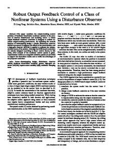
≤ βx˜ (2|x0 |, k) + βx˜ (2kek, 0) + γxe˜ (kek) + kek = βx (|x0 |, k) + γxe (kek). V. O UTPUT FEEDBACK CONTROL OF A B UCK -B OOST DC-DC CONVERTER In this section we illustrate Algorithm IV.1, where instead of xk we use xˆk for feedback. The estimate xˆk is generated by an observer having asymptotically stable error dynamics. The resulting output-based NMPC scheme is employed to control a Buck-Boost DC-DC converter power circuit. BuckBoost circuits are very important and they are widely used in relevant applications, ranging from hybrid and electric vehicles to solar plants, etc. An schematic view of the circuit is given in Fig. 1. A discrete-time nonlinear averaged model of the converter has been developed in [13], i.e. " # m + T xm − T (xm −V )um x in m m 1,k k L 2,k L 2,k xk+1 = , ym m + T xm um + (1 − T )xm k = x2,k , − CT x1,k C 1,k k RC 2,k (23)
3002
WeA12.5 where + Vin + −
ON/OFF (um )
L
C
R
x1m Fig. 1.
bx1 = 0.01 −
x2m
bx2 = −20 − x2ss ,
−
bu = 0.1 −
A schematic representation of a Buck-Boost converter.
m xm ]⊤ ∈ R2 , ym ∈ R and um ∈ R are the where xkm = [x1,k 2,k k k state the output and control, respectively. x1m represents the current flowing through the inductor, x2m the voltage across the capacitor and um represents the duty cycle (i.e. the fraction of the sampling period during which the transistor is kept ON). The sampling period T corresponds to a sampling frequency of 10[kHz], the inductance L = 4.2 × 10⁻³ [H], the capacitance C = 2200[µ F], the load resistance R = 165[Ω] and the source input voltage is equal to Vin = 15[V ]. The control objective is to reach a desired steady state value of the output voltage, i.e. x2ss , as fast as possible and with minimum m , overshoot. In practice only the output, i.e. output voltage x2,k is available for feedback, so output based controllers with a stability guarantee are needed. At the same time, constraints m must be fulfilled. The output based MPC on the current x1,k framework, as proposed in this paper, is used to design a controller for this task. From x2ss one can obtain the steady state duty cycle and inductor current as follows:
uss =
x2ss , ss x2 −Vin
x1ss =
x2ss . R(uss − 1)
(24)
Furthermore, the following physical constraints must be fulfilled at all times k ∈ Z+ : m x1,k ∈ [0.01, 5],
m x2,k ∈ [−20, 0],
um k ∈ [0.1, 0.6].
(25)
To implement the proposed MPC scheme we perform first the following coordinate transformation on (23) m x1,k = x1,k − x1ss ,
m x2,k = x2,k − x2ss ,
ss uk = um k −u .
1 ss ss 1 ss ss x x2 (x2 −Vin ), b 1 = 5 − x (x −Vin ), RVin RVin 2 2
(26)
and
u
b = 0.6 −
fz (yk−1 , yk , uk−1 , uk ) = with
The constants α , β , γ and δ depend on the fixed steady state value x2ss as follows
and
(( ( + 1− T ( RC )((
0
T T C ϖ +α yk−1 + β − L yk−1 uk−1 +γ uk T ϖ +γ u T k−1 + 1− RC yk−1 +δ ϖ +δ (ϖ +α yk−1 C T + β − L yk−1 uk−1
ϖ=
( (
)
(
)
)
)
) ) )
))
,
RC(yk − γ uk−1 − yk−1 ) + Tyk−1 , R(Tuk−1 + δ C) hz (zn,k ) = zn,k .
Using (26) and (24), the constraints given in (25) can be converted to: n o x x X = x ∈ R2 x1 ∈ [bx1 , b 1 ], x2 ∈ [bx2 , b 2 ] o n (28) u U = u ∈ R u ∈ [bu , b ] ,
x2ss . x2ss −Vin
The control objective can now be formulated as to stabilize (27) around the equilibrium (0, 0) while fulfilling the constraints given in (28). 1) Controller: The ISS (w.r.t. additive disturbances) NMPC scheme from Section IV is employed to design the NMPC controller. The method in [12] is applied to find a matrix PV which defines the� proposed � ISS Lyapunov function 0.1 0 V (x) = |P x|. For Q = V V 0 0.1 we have obtained PV = � 2.4545 4.9275 � . The employed NMPC costs defined by F and 5.6292 −6.0353 L are given as F = |Pxk+N|k | and L = |Qxk+i|k | + |Ru uk+i|k |. To achieve good performance, the �NMPC � cost� matrices � 0 , Q = 2 0 and have been chosen as follows: P = 50 10 06 Ru = 0.001. Further we chose the prediction horizon to be N = 5. To conclude about ISS w.r.t. ex (possibly induced by an observer) we rely on Theorem IV.5. 2) Observer: For the observer design we employ the proposed extended observer design methodology proposed in [14]. For the considered system, defined by f and g, we can obtain an observer with asymptotically stable error dynamics. Due to the scope of the paper and space limitations we will not go into further details concerning the observer design. For more details on the employed observer design methodology in relation to NMPC we refer the reader to [15], [16]. However, in order to provide the reader with results that can be reproduced, we give the functions that define an observer from the used observer design methodology, and refer to [15] for more details on this issue. The following functions fz and hz define the employed observer on the domain X × U
This is done in order to obtain a model of the form (8) with f (0, 0) = 0. We obtain then the following vector fields f and g, defining a nonlinear model of form (8): � � x + α x2,k + (β − TL x2,k )uk , f (xk , uk ) = T 1,k T ( C x1,k + γ )uk + (1 − RC )x2,k + δ x1,k (27) g(xk ) = x2,k .
xss T T α = (1 − ss 2 ), β = (Vin − x2ss ), L x2 −Vin L � � x2ss T T γ= x2ss (x2ss −Vin ) and δ = − 1 . RCVin C x2ss −Vin
x2ss x2ss −Vin
x
b 2 = −x2ss ,
(29)
For observer gains ℓ1 = 0.1 and ℓ2 = 0.1 we have an observer with asymptotically stable error dynamics. 3) Simulation: Simulation results for the closed-loop system, i.e. NMPC controller interconnected with the observer and the system, are given in Fig. 2 and Fig. ??. Note that although the NMPC controller and observer computations were performed for the transformed system, defined by (27), we chose to present all variables in Fig. 2 in original coordinates (corresponding to (23)), in order to preserve the
3003
WeA12.5 physical meaning of the results. For the obtained simulation the system was initialized with x0m = [0.01 0]T and the observer was initialized with zˆ0 = [0.1 0.2]T , u−1 = 0 and y−1 = 0 (see [14]). Note the estimation errors ex1 ,k and ex2 ,k converge to zero and the desired steady state value x2ss of system (23) is reached within reasonable time without any overshoot. Moreover, the constraints (25) are satisfied at all times.
0.6
Estimation error (x1 − xˆ1 ) inductor current
0.4
ex1
0.2 0
−0.2 −0.4 0
Duty cycle [-]
0.002 0.004 0.006 0.008
0.01
0.012 0.014 0.016 0.018
time [s]
0.6
0.4
Estimation error (x2 − xˆ2 ) output voltage
um 0.4
0.2
0.2
ex2 0
0.002
0.004
0.006
0.008
0.01
0.012
0.014
0.016
0.018
0
−0.2
Inductor current [A] −0.4
1.5
x1m
0
1
0.002 0.004 0.006 0.008
0.01
0.012 0.014 0.016 0.018
time [s] 0.5
Fig. 3. Estimation error trajectories (in x-coordinates) of the observer error dynamics.
0 0
0.002
0.004
0.006
0.008
0.01
0.012
0.014
0.016
0.018
Output voltage [V] 0 −1
x2m −2 −3 −4 0
0.002
0.004
0.006
0.008
0.01
0.012
0.014
0.016
0.018
time [s] Fig. 2. The state and control trajectories are represented by the solid lines. The dashed and dotted lines represent the constraints and the desired steady state values (x1ss = 0.0307[A], x2ss = −4[V ], uss = 0.2105[−]), respectively.
VI. C ONCLUSIONS We propose a framework for the design of (local) asymptotically stabilizing observer-based output feedback model predictive controllers for nonlinear discrete time Lipschitz continuous systems with input and state constraints. The main result on which the framework is based, is the ability to infer ISS with respect to measurement noise (e.g. presence of observer errors in the state) from ISS with respect to additive disturbances for the considered class of systems. Furthermore, a case study on the output-based control of a Buck-Boost DC-DC power converter is presented. References [1] D. Q. Mayne, J. B. Rawlings, C. V. Rao, and P. O. M. Scokaert, “Constrained model predictive control: stability and optimality,” Automatica, vol. 36, no. 6, pp. 789–814, June 2000. [2] P. O. M. Scokaert, J. B. Rawlings, and E. S. Meadows, “Discrete-time stability with pertubations: application to model predictive control,” Automatica, vol. 33, no. 3, pp. 463–470, March 1997. [3] L. Magni, G. De Nicolao, and S. R., “Output feedback recedinghorizon control of discrete-time nonlinear systems,” in the Proceedings of the IFAC Nonlinear Systems Design Symposium, Enschede, Netherlands, July 1998, pp. 422–427. [4] M. J. Messina, S. E. Tuna, and A. R. Teel, “Discrete-time certainty equivalence output feedback: allowing discontinuous control laws including those from model predictive control,” Automatica, vol. 41, no. 4, pp. 617–628, April 2005.
[5] R. Findeisen, L. Imsland, F. Allg¨ower, and B. A. Foss, “State and output feedback nonlinear model predictive control: An overview,” European Journal of Control, vol. 9, pp. 190–207, 2003. [6] V. Adetola and M. Guay, “Nonlinear sampled-data output feedback receding horizon control,” Journal of Process Control, vol. 15, no. 4, pp. 469–480, June 2005. [7] E. D. Sontag and Y. Wang, “New characterizations of the input to state property,” IEEE Transactions on Automatic Control, vol. 41, no. 9, pp. 1283–1294, September 1996. [8] Z. P. Jiang and Y. Wang, “Input-to-state stability for discrete-time nonlinear systems,” Automatica, vol. 37, no. 6, pp. 857–869, June 2001. [9] M. Lazar, W. P. M. H. Heemels, A. Bemporad, and S. Weiland, “On the stability and robustness of non-smooth nonlinear model predictive control,” in Workshop on Assessment and Future Directions of NMPC, Freudenstadt-Lauterbad, Germany, 2005, pp. 327–334. [10] S. S. Keerthi and E. G. Gilbert, “An existence theorem for discretetime infinite-horizon optimal control problems,” IEEE Transactions on Automatic Control, vol. AC-30, no. 9, pp. 907–909, 1985. [11] D. M. Limon, T. Alamo, and E. F. Camacho, “Input-to-stable MPC for constrained discrete-time nonlinear systems with bounded additive uncertainties,” in the Proceedings of the 41st IEEE Conference on Decision and Control, Las Vegas, Nevada, USA, December 2002, pp. 4619–4624. [12] M. Lazar, W. P. M. H. Heemels, B. J. P. Roset, H. Nijmeijer, and P. P. J. van den Bosch, “Input-to-state stabilizing sub-optimal NMPC with an application to DC-DC converters,” International Journal on Robust Nonlinear Control, 2007, accepted for publication. [13] M. Lazar and R. De Keyser, “Nonlinear predictive control of a DCto-DC converter.” in the Proceedings of the Symposium on Power Electronics, Electrical Drives, Automation & Motion, Capri, Italy, 2004. [14] T. Lilge, “On observer design for non-linear discrete-time systems,” European Journal of Control, vol. 4, pp. 306–319, 1998. [15] B. J. P. Roset, M. Lazar, W. P. M. H. Heemels, and H. Nijmeijer, “A stabilizing output based nonlinear model predictive control scheme,” in the Proceedings of 45th IEEE Conference on Decision and Control, San Diego, USA, December 2006, pp. 4627–4632. [16] ——, “Stabilizing output feedback nonlinear model predictive control: An extended observer approach,” submitted to a journal. To obtain a copy please contact the authors.
3004