Robust Model Predictive Control of Nonlinear Affine Systems. Based on a Two-layer Recurrent Neural Network. Zheng Yan and Jun Wang. AbstractâA robust ...
Proceedings of International Joint Conference on Neural Networks, San Jose, California, USA, July 31 – August 5, 2011
Robust Model Predictive Control of Nonlinear Affine Systems Based on a Two-layer Recurrent Neural Network Zheng Yan and Jun Wang
Abstract— A robust model predictive control (MPC) method is proposed for nonlinear affine systems with bounded disturbances. The robust MPC technique requires on-line solution of a minimax optimal control problem. The minimax strategy means that worst-case performance with respect to uncertainties is optimized. The minimax optimization problem involved in robust MPC is reformulated to a minimization problem and then is solved by using a two-layer recurrent neural network. Simulation examples are included to illustrate the effectiveness of the proposed method.
I. I NTRODUCTION
M
ODEL PREDICTIVE CONTROL (MPC) is a powerful technique for optimizing performance of control systems. MPC applies on-line optimization to the model of the system over a finite horizon of future time. By taking the current state as an initial state, an objective function is optimized at each sample time, and at the next computation time interval, the calculation is repeated with new state information. A sequence of control actions is calculated at each step, but only the first one is implemented. Comparing with many other control techniques, MPC has many desirable features for industrial applications, such as the ability to directly take into account input and output constraints, as well as the capacity to handle multivariable process control. In many control engineering applications, there are always two kinds of uncertainties in a system model. One is caused by the lack of information on the system’s structure and the other one is due to internal and external disturbance [1]. Consequently, the issue of robustness, i.e. the maintenance of certain properties such as performance and stability in the presence of model mismatch and disturbances, is of great importance [2][3][4]. One way to achieve robustness in MPC is the worst-case approach which obtains a sequence of control actions that minimize the worst-case control cost. The worst-case approach requires on-line solution of a minimax optimization problem [5]. Although robust MPC has been widely investigated in theory, most research accomplishments are conceptual controllers that are not suitable for hardware implementation [4][6]. Thus, further investigations on robust MPC controller are necessary. A key issue for robust MPC synthesis lies in on-line optimization. The effectiveness and efficiency of the optimization method determines whether the robust MPC techZheng Yan and Jun Wang are with the Department of Mechanical and Automation Engineering, The Chinese University of Hong Kong, Shatin, New Territories, Hong Kong (email: {zyan, jwang}@mae.cuhk.edu.hk). The work described in the paper was supported by the Research Grants Council of the Hong Kong Special Administrative Region, China, under Grants CUHK417209E and CUHK417608E.
978-1-4244-9636-5/11/$26.00 ©2011 IEEE
nique can be implemented successfully. In the past two decades, recurrent neural networks (RNNs) emerged as a promising computational approach for solving various online optimization problems. There are several advantages for choosing neural network approach: firstly, neural networks can solve problems with time-varying parameters; secondly, they can deal with large scale problems with high parallelizable ability; thirdly, they can be implemented in hardware. Many neural network models have been proposed in recent decade. By the duality and projection methods, Xia, Feng, Liu, Hu and Wang developed several neural networks for solving linear programming, quadratic programming, general convex programming and pseudoconvex optimization problems; such as the primal-dual network [7], the general projection neural network [8], the simplified dual network [9], and the improved dual neural network [10]. These recent neural networks have shown good performance in terms of global convergence and low computational complexity. Many attempts on incorporating neural networks with model predictive control have been made in last two decades. For example, an overview of how neural networks can be used in model predictive control is presented in [11]. In [12], a methodology to design and implement neural predictive controllers for nonlinear systems is discussed. In [13], a dual neural network is employed to deal with the multistage optimization problem involved in generalized predictive control algorithm. The use of neural networks can greatly improve the overall success of MPC implementation. In this paper, a robust MPC scheme on nonlinear affine system which can represent many industrial process models is proposed. An additive bounded disturbance is explicitly taken into consideration. We reformulate the minimax optimization problem to a nonlinear minimization problem. Then we apply a two-layer recurrent neural network model for solving such nonlinear programming problem. We apply the method on two typical industrial models to demonstrate the performance. The rest of this paper is organized as follows. In Section II, robust MPC of nonlinear affine system is formulated. In Section III, a recurrent network is presented to solve the optimization problem. In Section IV, numerical examples are provided. Finally, Section V concludes this paper. II. P ROBLEM F ORMULATION Consider the following discrete-time nonlinear affine system:
24
𝑥(𝑘 + 1) = 𝑓 (𝑥(𝑘)) + 𝑔 (𝑥(𝑘)) 𝑢(𝑘), 𝑦(𝑘) = 𝐶𝑥(𝑘) + 𝐷𝑤(𝑘).
(1)
with constraints:
Define the following vectors:
𝑢min ≤ 𝑢(𝑘) ≤ 𝑢max , Δ𝑢min ≤ Δ𝑢(𝑘) ≤ Δ𝑢max , 𝑤min ≤ 𝑤(𝑘) ≤ 𝑤max , 𝑦min ≤ 𝑦(𝑘) ≤ 𝑦max .
.. . 𝑦(𝑘 + 𝑁 ∣𝑘) =𝐶(𝑓 (𝑥(𝑘 + 𝑁 − 1∣𝑘 − 1)) + 𝑔(𝑥(𝑘 + 𝑁 − 1∣𝑘 − 1))(𝑢(𝑘 − 1) + Δ𝑢(𝑘∣𝑘)) + . . . + (5) Δ𝑢(𝑘 + 𝑁𝑢 − 1∣𝑘)) + 𝐷𝑤(𝑘 + 𝑁 ∣𝑘) 𝑇
𝑦¯(𝑘) = [𝑦(𝑘 + 1∣𝑘) . . . 𝑦(𝑘 + 𝑁 ∣𝑘)] ∈ ℜ𝑁 𝑝 𝑇
𝑢 ¯(𝑘) = [𝑢(𝑘∣𝑘) . . . 𝑢(𝑘 + 𝑁𝑢 − 1∣𝑘)] ∈ ℜ𝑁𝑢 𝑚 𝑇
(2)
𝑟¯(𝑘) = [𝑟(𝑘 + 1∣𝑘) . . . 𝑟(𝑘 + 𝑁 ∣𝑘)] ∈ ℜ𝑁 𝑝
where 𝑥(𝑘) ∈ ℜ𝑛 is the state vector, 𝑢(𝑘) ∈ ℜ𝑚 is the input vector, 𝑦(𝑘) ∈ ℜ𝑝 is the output vector, 𝑤(𝑘) ∈ ℜ𝑞 is the bounded disturbance vector, 𝑓 (⋅), 𝑔(⋅) are nonlinear functions, 𝐶 ∈ ℜ𝑝×𝑛 , and 𝐷 ∈ ℜ𝑝×𝑞 . 𝑢min ≤ 𝑢max , Δ𝑢min ≤ Δ𝑢max , 𝑦min ≤ 𝑦max , and 𝑤min ≤ 𝑤max are vectors of lower and upper bounds. MPC is an iterative optimization technique: at each sampling time 𝑘, measure or estimate the current state, and then obtain the optimal input vector by optimizing a control cost function. When bounded disturbances are explicitly considered, a robust MPC law can be derived by minimizing the maximum cost within the model described by the uncertainty set. The optimal control actions can be obtained by solving the following optimization problem repeatedly over 𝑘:
𝑥 ¯(𝑘) = [𝑥(𝑘 + 1∣𝑘) . . . 𝑥(𝑘 + 𝑁 ∣𝑘)] ∈ ℜ𝑁 𝑛
min max
Δ𝑢(𝑘) 𝑤(𝑘)
𝐽(Δ𝑢(𝑘), 𝑤(𝑘))
+
𝑁∑ 𝑢 −1 𝑗=0
(4) ∥Δ𝑢(𝑘 +
𝑇
Δ¯ 𝑢(𝑘) = [Δ𝑢(𝑘∣𝑘) . . . Δ𝑢(𝑘 + 𝑁𝑢 − 1∣𝑘)] ∈ ℜ𝑁𝑢 𝑚 𝑇
𝑤(𝑘) ¯ = [𝑤(𝑘 + 1∣𝑘) . . . 𝑤(𝑘 + 𝑁 ∣𝑘)] ∈ ℜ𝑁 𝑞 (6) where 𝑟¯(𝑘) is known in advance. The predicted output 𝑦¯(𝑘) is then expressed in the following form: ˜ 𝑤(𝑘) ˜ ˜ 𝑤(𝑘) 𝑦¯(𝑘) = 𝐶˜ 𝑥 ¯(𝑘)+𝐷 ¯ = 𝐶(𝐺Δ¯ 𝑢(𝑘)+𝑓˜+˜ 𝑔 )+𝐷 ¯ (7) ⎡
where
𝐶 ⎢ .. ˜ 𝐶 =⎣. ⎡
2 𝑗∣𝑘)∥𝑅
where 𝑟(𝑘 + 𝑗∣𝑘) denotes the reference of output signal, 𝑦(𝑘 + 𝑗∣𝑘) denotes the predicted output, and Δ𝑢(𝑘 + 𝑗∣𝑘) denotes the input increment, where Δ𝑢(𝑘 + 𝑗∣𝑘) = 𝑢(𝑘 + 𝑗∣𝑘) − 𝑢(𝑘 − 1 + 𝑗∣𝑘). 𝑁 and 𝑁𝑢 are prediction horizon (1 ≤ 𝑁 ) and control horizon (0 < 𝑁𝑢 ≤ 𝑁 ), respectively. 𝑄 2 and 𝑅 are appropriate weighting matrices. ∥⋅∥ denotes the Eulidean norm of the corresponding vector. The first term in (4) represents the error between the predicted output and the reference output while the second term considers the control effort. The previous obtained predicted states are used to estimate the state vectors. So, according to model (1), we have: 𝑦(𝑘 + 1∣𝑘) =𝐶(𝑓 (𝑥(𝑘∣𝑘 − 1)) + 𝑔(𝑥(𝑘∣𝑘 − 1))(𝑢(𝑘 − 1) + Δ𝑢(𝑘∣𝑘))) + 𝐷𝑤(𝑘 + 1∣𝑘) 𝑦(𝑘 + 2∣𝑘) =𝐶(𝑓 (𝑥(𝑘 + 1∣𝑘 − 1)) + 𝑔(𝑥(𝑘 + 1∣𝑘 − 1)) (𝑢(𝑘 − 1) + Δ𝑢(𝑘∣𝑘) + Δ𝑢(𝑘 + 1∣𝑘)))+ 𝐷𝑤(𝑘 + 2∣𝑘)
0
𝐷 ⎢ .. ˜ 𝐷=⎣.
(3)
subject to constraints (2). For model (1), the following cost function with finite horizon quadratic criterion can be used for calculation: 𝑁 ∑ 2 ∥𝑟(𝑘 + 𝑗∣𝑘) − 𝑦(𝑘 + 𝑗∣𝑘)∥𝑄 𝐽(Δ𝑢(𝑘), 𝑤(𝑘)) = 𝑗=1
𝑇
0
⎤ 0 .. ⎥ ∈ ℜ𝑁 𝑝×𝑁 𝑛 .⎦
... .. . ...
𝐶
... .. . ...
𝐷
⎡
𝑔(𝑥(𝑘∣𝑘 − 1)) ⎢ 𝑔(𝑥(𝑘 + 1∣𝑘 − 1)) 𝐺=⎢ .. ⎣ . 𝑔(𝑥(𝑘 + 𝑁 − 1∣𝑘 − 1))
⎤ 0 .. ⎥ ∈ ℜ𝑁 𝑝×𝑁 𝑞 .⎦ ... ... .. . ...
⎤ 0 0 ⎥ ⎥ .. ⎦ . 𝑔(𝑥(𝑘 + 𝑁 − 1∣𝑘 − 1))
∈ ℜ𝑁 𝑛×𝑁𝑢 𝑚
⎡
⎢ ⎢ 𝑓˜ = ⎢ ⎣ ⎡ ⎢ ⎢ 𝑔˜ = ⎢ ⎣
𝑓 (𝑥(𝑘∣𝑘 − 1)) 𝑓 (𝑥(𝑘 + 1∣𝑘 − 1)) .. .
⎤ ⎥ ⎥ ⎥ ∈ ℜ𝑁 𝑛 ⎦
𝑓 (𝑥(𝑘 + 𝑁 − 1∣𝑘 − 1)) 𝑔(𝑥(𝑘∣𝑘 − 1))𝑢(𝑘 − 1) 𝑔(𝑥(𝑘 + 1∣𝑘 − 1))𝑢(𝑘 − 1) .. .
⎤ ⎥ ⎥ ⎥ ∈ ℜ𝑁 𝑛 ⎦
𝑔(𝑥(𝑘 + 𝑁 − 1∣𝑘 − 1))𝑢(𝑘 − 1) Hence, the original optimization problem (3) becomes: 2 ˜ ˜ 𝑤(𝑘) min max ¯ 𝑟(𝑘) − 𝐶˜ 𝑓˜ − 𝐶˜ 𝑔˜ − 𝐶𝐺Δ¯ 𝑢(𝑘) − 𝐷 ¯ Δ¯ 𝑢(𝑘) 𝑤(𝑘) ¯
𝑄
+
2 ∥Δ¯ 𝑢(𝑘)∥𝑅
,
s.t. Δ¯ 𝑢min ≤ Δ¯ 𝑢(𝑘) ≤ Δ¯ 𝑢max , ˜ 𝑢 ¯min ≤ 𝑢 ¯(𝑘 − 1) + 𝐼Δ¯ 𝑢(𝑘) ≤ 𝑢 ¯max ,
˜ ˜ 𝑤(𝑘) 𝑢(𝑘) + 𝐷 ¯ ≤ 𝑦¯max , 𝑦¯min ≤ 𝐶˜ 𝑓˜ + 𝐶˜ 𝑔˜ + 𝐶𝐺Δ¯ 𝑤 ¯min ≤ 𝑤(𝑘) ¯ ≤𝑤 ¯max (8)
25
⎡
where
𝐼 ⎢𝐼 ⎢ 𝐼˜ = ⎢ . ⎣ ..
0 𝐼 .. .
... ... .. .
⎤ 0 0⎥ ⎥ 𝑁 𝑚×𝑁𝑢 𝑚 .. ⎥ ∈ ℜ 𝑢 .⎦
𝐼
𝐼
...
𝐼
⎡
⎤ 𝑏1 ⎢ Δ¯ ⎥ ⎢ 𝑢𝑚𝑎𝑥 ⎥ 4𝑁𝑢 𝑚+2𝑁 𝑝+2𝑁 𝑞 ⎥ 𝑤 ¯ 𝑏=⎢ . ⎢ 𝑚𝑎𝑥 ⎥ ∈ ℜ ⎣−Δ¯ 𝑢𝑚𝑖𝑛 ⎦ −𝑤 ¯𝑚𝑖𝑛
By defining 𝑢 = Δ¯ 𝑢(𝑘) ∈ ℜ𝑁𝑢 𝑚 , 𝑤 = 𝑤(𝑘) ¯ ∈ ℜ𝑁 𝑞 , problem (8) can be rewritten as the following minimax problem: [ ]𝑇 [ ] [ ]𝑇 [ ] 𝑢 𝑢 𝑐 𝑢 + 1 𝑊1 min max 𝑤 𝑤 𝑤 𝑐2 𝑢 𝑤 s.t. Δ¯ 𝑢min ≤ 𝑢 ≤ 𝑢 ¯max , ¯max , 𝑤 ¯min ≤ 𝑤 ≤ 𝑤 𝐸1 𝑢 ≤ 𝑏 1 . (9) where the coefficients are: [ 𝑇 𝑇 ˜ +𝑅 𝐺 𝐶˜ 𝑄𝐶𝐺 𝑊1 = 𝑇 ˜ 𝐷 𝑄𝐶𝐺
𝐺𝑇 𝐶˜ 𝑇 𝑄𝐷 𝐷𝑇 𝑄𝐷
]
𝑐1 = −2𝐺𝑇 𝐶˜ 𝑇 𝑄(¯ 𝑟(𝑘) − 𝐶˜ 𝑔˜ − 𝐶˜ 𝑓˜) ∈ ℜ𝑁𝑢 𝑚 , 𝑐2 = −2𝐷𝑇 𝑄(¯ 𝑟(𝑘) − 𝐶˜ 𝑔˜ − 𝐶˜ 𝑓˜) ∈ ℜ𝑁 𝑞 , ˜ − 𝐶𝐺
˜ 𝐶𝐺
]𝑇
∈ ℜ(2𝑁𝑢 𝑚+2𝑁 𝑝)×𝑁𝑢 𝑚 ,
⎤ ¯(𝑘 − 1) −¯ 𝑢min + 𝑢 ⎥ ⎢ ¯(𝑘 − 1) 𝑢 ¯max − 𝑢 ⎥ ∈ ℜ2𝑁𝑢 𝑚+2𝑁 𝑝 𝑏1 = ⎢ ⎣−¯ ¯ − 1)⎦ 𝑦min + 𝐶˜ 𝑓˜ + 𝐶˜ 𝑔˜ + 𝐷𝑤(𝑘∣𝑘 ¯ − 1) 𝑦¯max − 𝐶˜ 𝑓˜ − 𝐶˜ 𝑔˜ − 𝐷𝑤(𝑘∣𝑘 𝑣 = max 𝑧 𝑇 𝑊1 𝑧 + 𝑐˜𝑇 𝑧 𝑤
where [ ] [ ] 𝑐 𝑢 𝑧= ∈ ℜ𝑁𝑢 𝑚+𝑁 𝑞 and 𝑐˜ = 1 ∈ ℜ𝑁𝑢 𝑚+𝑁 𝑞 𝑐2 𝑤 The optimization problem (9) is then equivalent to: min s.t.
where
⎡
𝐸1 ⎢𝐼 ⎢ 𝐸2 = ⎢ ⎢0 ⎣−𝐼 0
𝑣 ][ ] [ ][ ] [ ]𝑇 [ 𝑊1 0 𝑧 𝑐˜ 𝑧 𝑧 + ≤0 0 0 𝑣 −1 𝑣 𝑣 [ ] [ ] 𝑧 𝐸2 0 ≤ 𝑏2 𝑣
𝛾𝑇 𝑠 𝑠𝑇 𝑊 𝑠 + 𝑐𝑇 𝑠 ≤ 0, 𝐸𝑠 ≤ 𝑏
(11)
where
𝐸 = [𝐸2
⎡
Let
min s.t.
𝛾 = [0, 0, . . . , 0, 1] ∈ ℜ𝑁𝑢 𝑚+𝑁 𝑞+1 , [ ] 𝑧 𝑠= ∈ ℜ𝑁𝑢 𝑚+𝑁 𝑞+1 , 𝑣 [ ] 𝑊1 0 𝑊 = ∈ ℜ(𝑁𝑢 𝑚+𝑁 𝑞+1)×(𝑁𝑢 𝑚+𝑁 𝑞+1) , 0 0 [ ] 𝑐˜ 𝑐= ∈ ℜ𝑁𝑢 𝑚+𝑁 𝑞+1 , −1
∈ ℜ(𝑁𝑢 𝑚+𝑁 𝑞)×(𝑁𝑢 𝑚+𝑁 𝑞) ,
[ 𝐸1 = −𝐼˜ 𝐼˜
Furthermore, the minimization problem (10) can be formulated as the following minimization problem subject to nonlinear inequality constraints:
(10)
⎤ 0 0⎥ ⎥ (4𝑁𝑢 𝑚+2𝑁 𝑝+2𝑁 𝑞)×(𝑁𝑢 𝑚+𝑁 𝑞) 𝐼 ⎥ , ⎥∈ℜ ⎦ 0 −𝐼
0] ∈ ℜ(4𝑁𝑢 𝑚+2𝑁 𝑝+2𝑁 𝑞)×(𝑁𝑢 𝑚+𝑁 𝑞+1) .
The solution to the minimization problem (11) gives the vector of control action Δ¯ 𝑢(𝑘) under the worst-case within the uncertainty domain. The optimal Δ¯ 𝑢(𝑘) can be used to calculate the optimal control input at time 𝑘. III. N EURAL N ETWORK A PPROACH Tank and Hopfiled first proposed a neural network for linear programming [14]. Their work has inspired many researchers to develop neural network models for solving linear and nonlinear optimization problems. Various neural network models have been developed for solving nonlinear optimization problems, e.g. [15][16][17]. In [15], Kennedy and Chua developed a penalty based network for solving nonlinear convex optimization programming, but the model cannot converge to an exact optimal solution due to the penalty parameter. In [16], a multi-layer recurrent neural is proposed for sovling convex quadratic programming problems. The network features global convergence property under weak conditions. In [17], a one-layer recurrent neural network with a discontinuous hard-limiting activation function is proposed for quadratic programming. In [18], Xia and Wang developed a recurrent neural network for nonlinear convex optimization problems. This neural network can handle nonlinear inequality constraints, and it is also shown to be Lyapunov stable and globally convergent to the optimal solution. We employ the proposed neural network here to solve (11).
26
Rewrite (11) in the general form: min
IV. S IMULATION E XAMPLES
𝑓 (𝑠) = 𝛾 𝑇 𝑠
s.t. 𝑐1 (𝑠) = 𝑠𝑇 𝑊 𝑠 + 𝑐𝑇 𝑠 ≤ 0, 𝑐2 (𝑠) = 𝐸𝑠 − 𝑏 ≤ 0
(12)
Because 𝑊1 in (9) is symmetric and positive definite, 𝑊 in (12) is symmetric and positive semi-definite. Thus 𝑐1 (𝑠) and 𝑐2 (𝑠) are both convex and twice differentiable. Problem (12) is shown to be a convex programming problem and it is suitable for applying the neural network presented in [18]. Then the Karush-Kuhn-Tucker (KKT) conditions for (12) can be represented as: 𝜆 ≥ 0, 𝑐(𝑠) ≤ 0, ∇𝑓 (𝑠) + ∇𝑐(𝑠)𝜆 ≥ 0, 𝜆𝑇 𝑐(𝑠) = 0.
(13)
4𝑁𝑢 𝑚+2𝑁 𝑝+2𝑁 𝑞+1
where 𝜆 ∈ ℜ is a dual variable for the 𝑇 corresponding Lagrangian function, 𝑐(𝑠) = [𝑐1 (𝑠) 𝑐2 (𝑠)] , ∇𝑐(𝑠) = (∇𝑐1 (𝑠), ∇𝑐2 (𝑠)) is the gradient of 𝑐(𝑠), and ∇𝑓 (𝑠) is the gradient of 𝑓 (𝑠). The Lagrangian function of (12) is defined as: 𝐿(𝑠, 𝜆) = 𝑓 (𝑠) + 𝜆𝑇 𝑐(𝑠)
(14)
As derived in [18], based on to the well-known saddle point theorem [19] and the projection theorem [20], a recurrent neural network model for solving (12) can be obtained, whose dynamic equations are: ( ) ( ) 𝑑 𝑠 −𝛼(∇𝑓 (𝑠) + ∇𝑐(𝑠)𝜆) = (15) 𝜖 −𝜆 + (𝜆 + 𝛼𝑐(𝑠))+ 𝑑𝑡 𝜆 = where 𝜖 and 𝛼 are positive constants, 𝜆+ + + + = 𝑚𝑎𝑥 {0, 𝜆𝑖 }. The ([𝜆1 ] , . . . , [𝜆𝑚 ] )𝑇 and [𝜆𝑖 ] presented neural network has single-layer structure with 5𝑁𝑢 𝑚 + 3𝑁 𝑞 + 2𝑁 𝑝 + 2 neurons in total and is suitable for hardware implementation. According to the stability analysis in [18], the neural network (15) is Lyapunov stable and globally convergent to the optimal solution. The MPC scheme for nonlinear affine systems based on the proposed recurrent neural network is summarized as follows: 1) Let 𝑘 = 1. Set control time terminal 𝑇 , prediction horizon 𝑁 , control horizon 𝑁𝑢 , sample period 𝜏 , weight matrices 𝑄 and 𝑅. ˜ 𝐷 ˜ and 2) Calculate process model matrices 𝐺, 𝑓˜, 𝑔˜, 𝐶, neural network matrices 𝑊 , 𝑐, 𝐸, 𝑏. 3) Solve the convex optimization problem (11) by using neural network (15) to obtain the optimal control action Δ¯ 𝑢(𝑘). 4) Calculate the optimal input vector 𝑢 ¯(𝑘) and implement 𝑢(𝑘∣𝑘). 5) If 𝑘 < 𝑇 , set 𝑘 = 𝑘 + 1, go to step 2; otherwise end.
In this section, two applications on industrial processes are provided to illustrate the performance of the proposed neural network based MPC method. Example 1: Nonlinear cooling continuous stirred tank reactor (CSTR) is a widely used process in chemical industry, whose dynamic model can be described as [21]: 𝑥2 𝑥2 𝛾
𝑥˙ 1 = −𝛼𝑥1 + 𝐷𝑎 (1 − 𝑥1 )𝑒 1+ 𝑥˙ 2 = −𝛼𝑥2 + 𝐵𝐷𝑎 (1 − 𝑥1 )𝑒
𝑥2 𝑥 1+ 2 𝛾
,
− 𝛽𝑥2 + 𝛽𝑢.
(16)
where 𝑥1 denotes the reactant concentration and 𝑥2 denotes the reactor temperature. Based on the aforementioned nonlinear MPC formulation and Euler discretization, we have: [ ] 0 𝑔= 𝛽 𝑓= ⎡
⎡
𝑥2 (𝑘) 𝑥2 (𝑘) 𝛾
⎤
⎤
⎢ ⎥ ⎦ 𝑥1 (𝑘) + 𝜏 ⎣−𝛼𝑥1 (𝑘) + 𝐷𝑎 (1 − 𝑥1 (𝑘))𝑒 ⎢ ⎥ ⎢ ⎥ ⎢ ⎥ ⎡ ⎤ 𝑥2 (𝑘) ⎢ ⎥ 𝑥2 (𝑘) ⎢ ⎥ ⎣𝑥2 (𝑘) + 𝜏 ⎣−𝛼𝑥2 (𝑘) + 𝐵𝐷𝑎 (1 − 𝑥1 (𝑘))𝑒 1+ 𝛾 − 𝛽𝑥2 (𝑘)⎦⎦ 1+
(17)
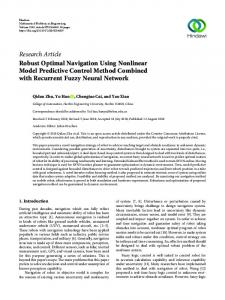
To conduct the numerical simulations, we set parameters 𝛼 = 1.0, 𝛽 = 0.3, 𝛾 = 20.0, 𝐵 = 1.0, 𝐷𝑎 = 0.072. An 𝑇 𝑇 uncertainty [−0.05 − 0.35] ≤ 𝑤 ≤ [0.05 0.35] is considered to affect system outputs. Let 𝐶 = 𝐼 and 𝐷 = 𝐼, so the outputs of CSTR model are: 𝑦1 (𝑘) = 𝑥1 (𝑘) + 𝑤1 (𝑘) and 𝑦2 (𝑘) = 𝑥2 (𝑘) + 𝑤2 (𝑘). The objective is to track the desired regulation trajectory given by [22] with the presence of disturbances: ⎧ ⎨ 0.4472, 𝑡 ≤ 15; 0.7646, 15 < 𝑡 < 30; 𝑟1 (𝑡) = ⎩ 0.4472, 30 ≤ 𝑡 < 45. ⎧ ⎨ 2.7520, 4.7052, 𝑟2 (𝑡) = ⎩ 2.7520,
𝑡 ≤ 15; 15 < 𝑡 < 30; 30 ≤ 𝑡 < 45.
(18)
The constraints are set as 7 ≤ 𝑢 ≤ 18, −1 ≤ Δ𝑢 ≤ 1, 0 ≤ 𝑦1 ≤ 0.85, 0 ≤ 𝑦2 ≤ 5. In the simulation, the initial 𝑇 states are [0, 0] , the prediction horizon and control horizon are 𝑁 = 5 and 𝑁𝑢 = 2, the weighting matrices are 𝑄 = 𝐼 and 𝑅 = 0.2𝐼. Sampling frequency is 10𝐻𝑧. In order to compare the effectiveness and efficiency of the proposed method, we also applied the control approach proposed in [23]. The simulation results are shown in Fig.1 - Fig.3. We can observe that the proposed approach resulted in much better tracking performance. The robustness of the controller is achieved by the proposed method. Example 2: Consider a quadruple-tank process described in [24] whose target is to control the level in the lower two
27
tanks with two pumps. The process model of the quadrupletank process is: 𝑎1 √ 𝑎3 √ 𝛾1 𝜌1 𝑥˙1 = − 2𝑔𝑥1 + 2𝑔𝑥3 + 𝑢1 , 𝐴1 𝐴1 𝐴1 √ √ 𝑎2 𝑎4 𝛾2 𝜌2 𝑥˙2 = − 2𝑔𝑥2 + 2𝑔𝑥4 + 𝑢2 , 𝐴2 𝐴2 𝐴2 𝑎3 √ (1 − 𝛾2 )𝜌2 2𝑔𝑥3 + 𝑢2 , 𝑥˙3 = − 𝐴3 𝐴3 𝑎4 √ (1 − 𝛾1 )𝜌1 2𝑔𝑥4 + 𝑢1 , 𝑥˙4 = − 𝐴4 𝐴1 𝑦1 = 𝜌𝑐 𝑥1 , (19) 𝑦2 = 𝜌𝑐 𝑥2 .
Output 1 0.8 0.7 0.6 0.5
y1
0.4 0.3 0.2 0.1
Proposed method Reference Method in [23] with lower bound w Method in [23] with upper bound w
0 −0.1
0
5
10
Fig. 1.
15
20 25 Time (s)
30
35
40
45
First output response in example 1
Output 2 5 4.5 4 3.5
y
2
3
𝑟2 (𝑡) = 6.3.
2.5
1.5 1
Reference Proposed method Method in [23] with lower bound w Method in [23] with upper bound w
0.5 0
5
10
Fig. 2.
15
20 25 Time (s)
30
35
40
45
Second output response in example 1
Control action 20
u
15
10
5
0
5
10
15
20 25 Time (s)
30
35
40
45
0
5
10
15
20 25 Time (s)
30
35
40
45
1
Δu
0.5
0
−0.5
(21) 𝑇
2
0
where 𝑥𝑖 is the water level in tank 𝑖, 𝑢1 and 𝑢2 are input voltages to the pumps, and 𝑦1 and 𝑦2 are output voltages. The parameters are set as: cross section of tank 𝐴1 = 𝐴3 = 28, 𝐴2 = 𝐴4 = 32; cross section of the outlet hole 𝑎1 = 𝑎3 = 0.071, 𝑎2 = 𝑎4 = 0.057; gravitational acceleration 𝑔 = 9.81; the fraction of water flowing to tank from pump 𝛾1 = 0.7, 𝛾2 = 0.6; gains 𝜌1 = 3.33, 𝜌2 = 3.35, 𝜌𝑐 = 0.5. Assume a disturbance −0.5 ≤ 𝑤 ≤ 0.5 affects both outputs. The objective to to track the reference given by [24] with the presence of disturbance: { 6.2, 𝑡 ≤ 20; (20) 𝑟1 (𝑡) = 7.1, 𝑡 > 20;
Fig. 3.
Control actions in example 1
The initial states are [12.4, 12.7, 1.8, 1.4] , the prediction horizon and control horizon are 𝑁 = 10 and 𝑁𝑢 = 2, the weighting matrices are 𝑄 = 𝐼 and 𝑅 = 0.1𝐼. Sampling frequency is 1𝐻𝑧. The MPC approach in [23] is also applied to this example to compare the performance. At time 𝑘 = 50, a step load disturbance enters in 𝑦2 . From the simulation results in Fig.4 - Fig.6, it can be seen that the proposed method herein resulted in much better control performance. The outputs track the references much faster and more stable compared with the other approach. V. C ONCLUSIONS In this paper, a robust MPC approach based on a recurrent neural network is proposed. An additive bounded disturbance is explicitly considered for nonlinear affine systems. The worst-case approach is adopted to obtain the optimal control actions. The original minimax optimization problem is reformulated to a nonlinear convex minimization problem. A recurrent neural network is applied for solving the reformulated optimization problem. Two simulation examples have demonstrated the usefulness of the proposed approach. With the recurrent neural network’s parallelizable ability, the proposed approach can be further applied in many large-scale multi-variable industrial processes. R EFERENCES [1] H. Khaloozadeh, M. Nekoui, F. Shahni “Adaptive tracking and asymptotic rejection of unknown but bounded disturbances in nolinear MIMO systems,” International Journal of Control, Automation, and Systems, vol. 8, no. 3, pp. 527-533, 2010.
28
Output 1 7.2 7
6.6
y
1
6.8
6.4 6.2 Proposed method Method in [23] with lower extreme w Method in [23] with upper extreme w
6 5.8
0
50
100
150
200
250
Time (s)
Fig. 4.
Output response in tank 1 in example2
Output 2 7
y
2
6.5
6
Proposed method Method in [23] with lower extreme w Method in [23] with upper extreme w 5.5
0
50
100
150
200
250
Time (s)
Fig. 5.
Output response in tank 2 in example 2
Control input 2.2
u
1
2 1.8 1.6 1.4
0
50
100
150
200
250
150
200
250
Time (s) 4
u
2
3.5
3
2.5
0
50
100 Time (s)
Fig. 6.
[2] S. J. Qin and Thomas A. Badgwell, “A survey of industrial model predictive control technology,” Control Engineering Practice, vol. 11, pp. 734-764, 2003. [3] M.Cannon and B. Kouvaritakis, Non-Linear Predictive Control: Theory &Practice. The Institution of Engineering and Technology Press, 2001. [4] D. Mayne, J. Rawlings, C. Rao, P. Scokaert “Constrained model predictive control: stability and optimality,” Automatica, vol. 36, no. 6, pp. 789-814, 2000. [5] J. Lofberg, Minimax Approaches to Robust Model Predictive Control. Ph.D. Thesis, Linkoping University, 2003 [6] Y. Pan and J. Wang, “Robust model predictive control using a discrete-time recurrent neural network,” Advances in Neural Networks - ISNN2008, Lecture Notes in Computer Sciences 5263, pp. 883-892, Springer-Verlag, 2008. [7] Y. Xia, G. Feng, and J. Wang, “A primal-dual neural network for on-line resolving constrained kinematic redundancy in robot motion control,” IEEE Transactions on Systems, Man and Cybernetics - Part B: Cybernetics, vol. 35, no. 1, pp. 54-64, 2005. [8] Y. Xia and J. Wang, “A general projection neural network for solving optimization and related problems,” IEEE Transactions on Neural Networks, vol. 15, pp. 318-328, 2004. [9] S. Liu and J. Wang, “A simplified dual neural network for quadratic programming with its KWTA application,” IEEE Transactions on Neural Networks, vol. 17, no. 6, pp. 1500-1510, 2006. [10] X. Hu and J. Wang, “An improved dual neural network for solving a class of quadratic programming problems and its k-winners-take-all application,” IEEE Transactions on Neural networks, vol. 19, no. 12, pp. 2022-2031, 2008. [11] M. Hagan, H. Demuth, O. Jesus, “An introduction to the use of neural networks in control systems,” International Journal of Robust and Nonlinear Control, vol. 12, no. 11, pp. 959-985, 2002. [12] M. Lazar and O. Pastravanu, “A neural predictive controller for nonlinear systems,” Mathematics and Computers in Simulation, vol. 60, no. 3-5, pp. 315-324, 2002. [13] L. Cheng, Z. Hou, M. Tan, “Constrained multi-variable generalized predictive control using a dual neural network,” Neural Computing and Applications, vol. 16, no. 6, pp. 505-512, 2007. [14] D. Tank and J. Hopfield, “Simple neural optimization networks: An A/D converter, signal decision circuit, and a linear programming circuit,” IEEE Transactions on Circuits and Systems, vol. CAS-33, pp. 533-541, 1986. [15] M. Kennedy and L. Chua, “Neural networks for nonlinear programming,” IEEE Transactions on Circuits and Systems., vol. 35, pp. 554562, 1988. [16] X. Hu and B. Zhang, “A new recurrent neural network for solving convex quadratic programming problems with an application to the kwinners-take-all problem,” IEEE Transactions on Neural Networks, vol. 20, no. 4, pp. 654-664, 2009. [17] Q. Liu and J. Wang, “A one-layer recurrent neural network with a discontinuous hard-limiting activation function for quadratic programming,” IEEE Transactions on Neural Networks, vol. 19, no. 4, pp. 558570, 2008. [18] Y. Xia and J. Wang, “A recurrent neural network for nonlinear convex optimization subject to nonlinear inequality constraints,” IEEE Transactions on Circuits and Systems - Part I: Regular Papers, vol. 51, no. 7, pp. 1385-1394, 2004. [19] M. Bazaraa, H. Sherali and C. Shetty Nonlinear Programming: Theory and Algorithms. New York: Wiley, 1993. [20] D. Kinderlehrer and G. Stampacchia, An Introduction to Variational Inequalities and Their Applications. New York: Academic, 1980. [21] A. Uppal, W.Ray, A. Poore, “On the dynamic behavior of continuous stirred tanks,” Chemical Engineering Science, vol. 29, pp. 957-985, 1974. [22] A. Soukkou, A. Khellaf, S. Leulmi, K. Boudeghdegh, “Optimal control of a CSTR process,” Brazilian Journal of Chemical Engineering, vol. 25, no. 4, pp. 799-812, 2008. [23] Y. Pan and J. Wang, “Model predictive control for nonlinear affine systems based on the simplified dual neural network,” IEEE International Symposium on Intelligent Control, pp 683-688, 2009. [24] K. Johansson, “The quadruple-tank process: a multivariable laboratory with an adjustable zero,” IEEE Transactions on Circuits and Systems, vol. 40, no. 9, pp. 621-626, 1993.
Control inputs in example 2
29