Design Principles of Wireless Sensor Networks Protocols for ... - DiVA

Chapter 9

Design Principles of Wireless Sensor Networks Protocols for Control Applications Carlo Fischione, Pangun Park, Piergiuseppe Di Marco, and Karl Henrik Johansson

Abstract Control applications over wireless sensor networks (WSNs) require timely, reliable, and energy efficient communications. This is challenging because reliability and latency of delivered packets and energy are at odds, and resource constrained nodes support only simple algorithms. In this chapter, a new system-level design approach for protocols supporting control applications over WSNs is proposed. The approach suggests a joint optimization, or co-design, of the control specifications, networking layer, the medium access control layer, and physical layer. The protocol parameters are adapted by an optimization problem whose objective function is the network energy consumption, and the constraints are the reliability and latency of the packets as requested by the control application. The design method aims at the definition of simple algorithms that are easily implemented on resource constrained sensor nodes. These algorithms allow the network to meet the reliability and latency required by the control application while minimizing for energy consumption. The design method is illustrated by two protocols: Breath and TREnD, which are implemented on a test-bed and compared to some existing solutions. Experimental results show good performance of the protocols based on this design methodology in terms of reliability, latency, low duty cycle, and load balancing for both static and time-varying scenarios. It is concluded that a system-level design is the essential paradigm to exploit the complex interaction among the layers of the protocol stack and reach a maximum WSN efficiency. Keywords Wireless sensor networks ( Networked Control ( IEEE 802.15.4 ( Optimization

C. Fischione (!) ACCESS Linnaeus Center, Electrical Engineering, Royal Institute of Technology, Stockholm, Sweden e-mail: [email protected]

S.K. Mazumder (ed.), Wireless Networking Based Control, DOI 10.1007/978-1-4419-7393-1 9, c Springer Science+Business Media, LLC 2011 !

203

204

C. Fischione et al.

9.1 Introduction Wireless sensor networks (WSNs) are networks of tiny sensing devices for wireless communication, actuation, control, and monitoring. Given the potential benefits offered by these networks, e.g., simple deployment, low installation cost, lack of cabling, and mobility, they are specially appealing for control applications in home and industrial automation [1–3]. The variety of application domains and theoretical challenges for WSNs has attracted research efforts for more than one decade. Nevertheless, a lively research and standardization activity is ongoing [2–5] and there is not yet a widely accepted protocol stack for WSNs for control applications. The lack of efficient protocol solutions is due to that the protocols for control applications face complex control and communication requirements. Traditional control applications are usually designed by a top-down approach from a protocol stack point of view, whereby most of the essential aspects of the network and sensing infrastructure that has to be deployed to support control applications are ignored. Here, packet losses and delays introduced by the communication network are considered as nonidealities and uncertainties and the controllers are tuned to cope with them without having any influence on them. The top-down approach is limited for two reasons: (1) it misses the essential aspect of the energy efficiency that is usually required to WSNs [2], and (2) it can be quite conservative and therefore inefficient, because the controllers are built by presuming worst case wireless channel conditions that may be rarely experienced in the reality. On the other side, protocols for WSNs are traditionally designed to maximize the reliability and minimize the delay. This is a bottom-up approach, where controller specifications are not explicitly considered even though the protocols are used for control. This approach is energy inefficient because high reliability and low latency may demand significant energy consumption [2, 6]. Therefore, it follows that there is the essential need of a new design approach. Traditional WSNs applications (e.g., monitoring) need a high probability of success in the packet delivery (reliability). In addition to reliability, control applications ask also for timely packet delivery (latency). If reliability and latency constraints are not met, the correct execution of control decisions may be severely compromised, thus creating unstable control loops [7]. High reliability and low latency may demand significant energy expenditure, thus reducing the WSN lifetime. Controllers can usually tolerate a certain degree of packet losses and delay [8]: For example, the stability of a closed-loop control system may be ensured by high reliable communications and large delays, or by low delays when the packet loss is high. In contrast to monitoring applications, for control applications there is no need to maximize the reliability. A tradeoff between latency, packet losses, and stability requirements can be exploited for the benefit of the energy consumption, as proposed by the system-level design approach [9]. Therefore, we claim that the protocol design for control needs a system-level approach whereby the need of a parsimonious use of energy and the typical requirements of the control applications are jointly taken into account and control and WSNs protocols are co-designed.

9

Design Principles of WSNs Protocols for Control Applications

205

Exploiting such a tradeoff poses extra challenges when designing WSNs protocols for control applications when compared to more traditional communication networks, namely: " Reliability: Sensor information must be sent to the sink of the network with a

"

"

"

"

given probability of success, because missing these data could prevent the correct execution of control actions or decisions concerning the phenomena sensed. However, maximizing the reliability may increase substantially the network energy consumption [2]. Hence, the network designers need to consider the tradeoff between reliability and energy consumption. Latency: Sensor information must reach the sink within some deadline [6]. A probabilistic delay requirement must be considered instead of using average packet delay since the delay jitter can be too difficult to compensate for, especially if the delay variability is large [10]. Retransmission of old data to maximize the reliability may increase the delay and is generally not useful for control application [7]. Energy efficiency: The lack of battery replacement, which is essential for affordable WSN deployment, requires energy-efficient operations. Since high reliability and low delay may demand a significant energy consumption of the network, thus reducing the WSN lifetime, the reliability and delay must be flexible design parameters that need to be adequate for the requirements. Note that controllers can usually tolerate a certain degree of packet losses and delay [8–12]. Hence, the maximization of the reliability and minimization of the delay are not the optimal design strategies for the control applications we are concerned within this chapter. Adaptation: The network operation should adapt to application requirement changes, varying wireless channel and network topology. For instance, the set of control application requirements may change dynamically and the communication protocol must adapt its design parameters according to the specific requests of the control actions. To support these changing requirements, it is essential to have an analytical model describing the relation between the protocol parameters and performance indicators (reliability, delay, and energy consumption). Scalability: Since the processing resources are limited, the protocol procedures must be computationally light. These operations should be performed within the network to avoid the burden of too much communication with a central coordinator. This is particularly important for large networks. The protocol should also be able to adapt to size variation of the network for example, caused by moving obstacles, or addition of new nodes.

In this chapter, we propose a design methodology for WSNs protocols for control application that embraces the issues mentioned above. The remainder of the chapter is organized as follows: in Sect. 9.2, we discuss the related literature. In Sect. 9.3, we describe the design method. Such a method is then applied in Sect. 9.4, where the Breath protocol is described and experimentally evaluated, and in Sect. 9.5, where the TREnD protocol is described and experimentally tested. In Sect. 9.6, we conclude the chapter.

206

C. Fischione et al.

9.2 Background Although the standardization process for WSNs is ongoing, there is not any widely accepted complete protocol stack for WSNs for control [2]. The IEEE 802.15.4 protocol [4], which specifies physical layer and medium access control (MAC), is the base of recent solutions in industrial environments as WirelessHART [13], ISA100 [2], and ROLL [5]. Hence, we consider IEEE 802.15.4 as the reference standard in our investigation. There have been many contributions to the problem of protocol design for WSNs, both in academia (e.g., [2, 14]) and in industry (e.g., [15–17]). New protocols have been built around standardized low-power protocols, such as IEEE 802.15.4 [4], Zigbee [18], and WirelessHART. WirelessHART is a promising solution for the replacement of the wired HART protocol in industrial contexts. However, the power consumption is not a main concern in WirelessHART, whereas the data link layer is based on Time Division Multiple Access (TDMA), which requires time synchronization and pre-scheduled fixed length time-slots by a centralized network manager. Such a manager should update the schedule frequently to consider reliability and delay requirements and dynamic changes of the network, which demands complex hardware equipments. WirelessHART is thus in contrast with the necessity of simple protocols able to work with limited energy and computing resources. In Table 9.1, we summarize the characteristics of the protocols that are relevant to the category of applications we are concerned with in this chapter. In the table, we have evidenced whether indications as energy E, reliability R, and delay D have been included in the protocol design and validation, and whether a cross-layer approach has been adopted. We discuss these protocols in the following.

Table 9.1 Protocol comparison. The letters E, R, and D denote energy, reliability, and communication delay Protocol E R D Layer GAF [19] ! & & bridge SPAN [20] ! & & bridge XMAC [21] ˚ & & MAC Flush [23] ˚ MAC Fetch [25] & ˚ & phy, MAC, routing GERAF [27] ! ! MAC, routing Dozer [26] ˚ ˚ MAC, routing MMSPEED [28] ! ! routing Breath ˚ ˚ ˚ phy, MAC, routing TREnD ˚ ˚ ˚ phy, MAC, routing

The circle denotes that a protocol is designed by considering the indication of the column, but it has not been validated experimentally. The circle with plus denotes that the protocol is designed by considering the indication and experimentally validated. The dot denotes that the protocol design does not include indication and hence cannot control it, but simulation or experiment results include it. The term “bridge” means that the protocol is designed by bridging MAC and routing layers

9


207

GAF [19], SPAN [20], and X-MAC [21] consider the energy efficiency as a performance indicator, which is attained by algorithms under the routing layer and above the MAC layer so-called bridge layer. Simulation results of reliability and delay are reported in [19,20]. These protocols have not been designed out of an analytical modeling of reliability and delay, so there is not systematic control of them. One of the first protocol for WSNs designed to offer a high reliability is RMST [22], but energy consumption of the network or delay have not been accounted for in this protocol. The same lack of energy efficiency and delay requirements can be found in the reliable solutions presented in [23–25]. Dozer [26] comprises the MAC and routing layer to minimize the energy consumption while maximizing the reliability of the network, but an analytical approach has not been followed. Specially, Fetch [25] and Dozer [26] are designed for monitoring application, which mainly deals with lower traffic load than control applications. The latency of Fetch [25] is significantly dependent on the depth of the routing tree and is around some hundred seconds. In addition, experimental results of Dozer [26] show good energy efficiency and reliability under very low traffic intensity (with data sampling interval of 120 s) but the delay in the packet delivery is not considered, which is essential for control applications [7, 8]. Energy efficiency with delay requirement for MAC and randomized routing is considered in GERAF [27], without simulation or experimental validation. The focuses of the protocols mentioned above [19–27] are the maximization of the energy efficiency or reliability, or just minimization of the delay, without considering simultaneously application requirements in terms of reliability and delay in the packet delivery. In other words, these protocols are mostly designed for monitoring applications and do not support typical control application requirements. Control and industrial applications are able to cope with a certain degree of packet losses and delay [8, 10, 11], which implies that the approaches followed in the protocols mentioned above are not the ideal solution for these applications. The maximization of the energy efficiency and reliability may give a long delay, which are bad for the stability of the closed-loop control system. Analogously, the maximization of the reliability may be energy demanding and may give long delay, all of which are not tolerable for control applications. In addition, the protocols mentioned above do not support an adaptation to the changes of the reliability and delay, which may be required by the controllers. The protocols MMSPEED [28] and SERAN [9] are appealing for control and industrial applications. However, MMSPEED is not energy efficient because it considers a routing technique with an optimization of reliability and delay without energy constraints. The protocol satisfies a high reliability requirement by using duplicated packets over multi-path routing. Duplicated packets increase the traffic load with negative effect on the stability and energy efficiency of the network. In SERAN, a system-level design methodology has been presented for industrial applications, but even though SERAN allows the network to operate with low energy consumption subject to delay requirements, it considers neither tunable reliability requirements nor duty-cycling policies, which are essential to

208

C. Fischione et al.

reduce energy consumption. Furthermore, SERAN focuses on low-traffic networks. These characteristics limit the performance of SERAN in terms of both energy and reliability in our application setup. Given the availability of numerous techniques to reduce energy consumption and ensure reliability and low delays, a cross-layer optimization is a natural approach for WSNs protocols. Some cross-layer design challenges of the physical, MAC, and network layers to minimize the energy consumption of WSNs have been surveyed in [29–31]. However, many of the cross-layer solutions proposed in the literature are hardly useful for the application domain we are targeting, because they require sophisticated processing resources, or instantaneous global network knowledge, which are out of the capabilities of real nodes. Moreover, the requirements of the control applications are not taken into account. In the following sections, we present a general approach to the design of WSNs protocols for control. We illustrate this approach by the protocols Breath and TREnD, which are presented in this chapter. These protocols embrace simultaneously the physical layer, the MAC layer, the networking layer, and the control application layer, see Table 9.1.

9.3 Protocol Design for Control Applications In this chapter, we are concerned with the design of protocols for WSNs used to close the loop between plants and controllers, see Fig. 9.1. The nodes connected to the plants take state information and transmit it to the sink via a multi-hop WSN. The controllers are attached to the sink of the network. The sink must receive packets from the nodes of the plants with a desired probability of success and within a latency constraint demanded by the controllers so that the control decision can be correctly taken. We assume that the communication network must be energy efficient to guarantee a long network lifetime. node 1 plant 1

controller 1 node 2 sink

plant 2

controller 2

WSN

node n

controller n

plant n

Fig. 9.1 Control over a wireless sensor network. There are n plants and n controllers. A network closes the loop from sensors attached to plants to the controllers

9


209

Give the system model reported in Fig. 9.1, we formulate the new WSNs protocol design approach for control applications by the following optimization problem, where the parameters of the physical layer, the MAC layer, the networking layer, and the control application layer are co-designed by a joint optimization: min x

s.t.

Etot .x/

(9.1a)

i D 1; : : : ; n; Ri .x/ & ˝i ; PrŒDi .x/ % !i # & 6i i D 1; : : : ; n;

(9.1b) (9.1c)

Each decision variable is a protocol parameter. These decision variables are denoted by the vector x, which can include the radio power used by the nodes, the MAC parameters (e.g., the access probability or the TDMA slot duration, or the random backoff of IEEE 802.15.4 MAC, etc.), and the routing parameters. Etot .x/ is the total energy consumption of the network, which is obviously function of the protocol parameters. Ri .x/ is the probability of successful packet delivery (reliability) from node i to the sink, and ˝i is the minimum desired probability. Di .x/ is a random variable describing the delay to transmit a packet from node i to the sink. !i is the desired maximum delay, and 6i is the minimum probability with which such a maximum delay should be achieved. Notice that Etot .x/, Ri .x/, Di .x/, i D 1; : : : ; n, are implicit functions of the wireless channel, network topology, and traffic load generated by the nodes. We remark that !i , 6i , and ˝i are the control requirements, and x collects the protocol parameters that must be adapted to the wireless channel conditions, network topology, and the control requirements for an efficient network operation. Since controllers may need some reliability and latency during certain time intervals, and a different pair of requirements during some other time intervals, the reliability and latency requirements may change dynamically depending on the state of the plant and the history of the control actions. This means that problem (9.1) must be solved periodically and nodes need to know the optimal solution to adapt their protocol operation so that a global optimum can be achieved. It follows that the proposed design method allows us to perform a systematic co-design between the control requirements of the application and the network energy consumption. Note that problem (9.1) can be a mixed integer-real optimization problem, because some of the protocol parameters can take on integer values. The solution to this problem can be obtained at the sink node, or by distributed algorithms, where each node performs local computation to achieve the optimal global solution. However, as it was noted in [32], the complex interdependence of the decision variables (sleep disciplines, clustering, MAC, routing, power control, etc.) lead to difficult optimization problems even in simple network topologies, where the analytical relations describing reliability, latency, and energy consumption may be highly nonlinear expressions. Such a difficulty is further exacerbated when considering non-TDMA scheme [33]. We propose a design approach that offers a computationally attractive solution by simplifications of adequate accuracy. We show how to model the relations of problem (9.1) and compute the solution to the problem in

210

C. Fischione et al.

the following two sections. Specifically, in Sect. 9.4 we apply this design method to a system where there is only a plant that needs to be controlled over a multi-hop network, whereas in Sect. 9.5, the design method is applied to a system where there are multiple plants.

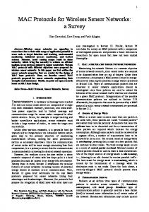
9.4 Breath The Breath protocol is designed for the scenario depicted in Fig. 9.2, where a plant is remotely controlled over a WSN [7, 11]. Outputs of the plant are sampled at periodic intervals by the sensors with total packet generation rate of & pkt/s. We assume that packets associated with the state of the plant are transmitted to a sink, which is connected to the controller, over a multi-hop network of uniformly and randomly distributed relaying nodes. No direct communication is possible between the pant and the sink. Relay nodes forward incoming packets. When the controller receives the measurements, they are used in a control algorithm to compensate the control output. The control law induces constraints on the communication delay and the packet loss probability. Packets must reach the sink within some minimum reliability and maximum delay. The application requirements are chosen by the control algorithm designers. Since they can change from one control algorithm to another, or a control algorithm can ask to change the application requirements from time to time, we allow them to vary. We assume that nodes of the network cannot be recharged, so the operations must conserve energy. The system scenario is quite general, because it applies to any interconnection of a plant by a multi-hop WSN to a controller tolerating a certain degree of data loss and delay [8–12]. A typical example of the scenario described above is an industrial control application. In particular, a WSN with nodes uniformly distributed in the environment (e.g., in the ceiling) can be deployed as the network infrastructure that support the

Controller

Plant

Network Sink

Relays

Cluster 1 Cluster 2

Edge

Cluster h-1 Cluster h

Fig. 9.2 Wireless control loop. An wireless network closes the loop from sensors to controller. The network includes nodes (black dots) attached to the plant, h # 1 relay clusters (grey dots), and a sink (black rectangular) attached to the controller. Note that the lines between the sink and the controller, and between the controller and the plant are not communication links, but control links

9


211

control of the state of the robots in a manufacturing cell [13, 34]. Typically, a cell is a stage of an automation line. Its physical dimensions range around 10 or 20 m on each side. Several robots cooperate in the cell to manipulate and transform the same production piece. Each node senses the state and has to report the data to the controller within a maximum delay. The decision making algorithm runs on the controller, which is usually a processor placed outside the cell. Multi-hop communication is needed to overcome the deep attenuations of the wireless channel due to moving metal objects and save energy consumption. The Breath protocol groups all N nodes between the cluster of nodes attached to the plan and the sink with h $ 1 relay clusters. Data packets can be transmitted only from a cluster to the next cluster closer to the sink. Clustered network topology is supported in networks that require energy efficiency, since transmitting data through relays consumes less energy than routing directly to the sink [35]. In [36], a dynamic clustering method adapts the network parameters. In [35] and [37], a cluster header is selected based on the residual energy levels for clustered environments. However, the periodic selection of clustering may not be energyefficient, and does not ensure the flexibility of the network to a time-varying wireless channel environment. A simpler geographic clustering is instead used in Breath. Nodes in the forwarding region send short beacon messages when they are available to receive data packets. Beacon messages are exploited to carry information related to the control parameters of the protocol. In the following sections, we will describe the protocol stack and state machine of Breath in Sects. 9.4.1 and 9.4.2, respectively.

9.4.1 The Breath Protocol Stack Breath uses a randomized routing, a hybrid TDMA at the MAC, radio power control at the physical layer, and sleeping disciplines. We give details in the following. In many industrial environments, the wireless conditions vary heavily because of moving metal obstacles and other radio disturbances. In such situations, routing schemes that use fixed routing tables are not able to provide the flexibility over mobile equipments, physical design limitations, and reconfiguration typical of an industrial control application. Fixed routing is inefficient in WSNs due to the cost of building and maintaining routing tables. To overcome this limitation, routing through a random sequence of hops has been introduced in [27]. The Breath protocol is built on an optimized random routing, where next hop route is efficiently selected at random. Randomized routing allows us to reduce overhead because no node coordination or routing state needs to be maintained by the network. Robustness to node failures is also considerably increased by randomized routing. Therefore, nodes route data packets to next-hop nodes randomly selected in a forwarding region. Each node, either transmitter or receiver, does not stay in an active state all time, but goes to sleep for a random amount of time, which depends on the traffic and channel conditions. Since traffic, wireless channel, and network topology may be

212

C. Fischione et al.

timevarying, the Breath protocol uses a randomized duty-cycling algorithm. Sleep disciplines turn off a node whenever its presence is not required for the correct operation of the network. GAF [19], SPAN [20], and S-MAC [38] focus on controlling the effective network topology by selecting a connected set of nodes to be active and turning off the rest of the nodes. These approaches require extra communication, since nodes maintain partial knowledge of the state of their individual neighbors. In Breath, each node goes to sleep for an amount of time that is a random variable dependent on traffic and network conditions. Let /c be the cumulative wake-up rate of each cluster, i.e., the sum of the wake-up rates that a node sees from all nodes of the next cluster. The cumulative wake-up rate of each cluster must be the same for each cluster to avoid congestions and bottlenecks. The MAC of Breath is based on a CSMA/CA mechanism similar to IEEE 802.15.4. Both data packets and beacon packets are transmitted using the same MAC. Specifically, the CSMA/CA checks the channel activity by performing clear channel assessment (CCA) before the transmission can commence. Each node maintains a variable NB for each transmission attempt, which is initialized to 0 and counts the number of additional backoffs the algorithm does while attempting the current transmission of a packet. Each backoff unit has duration Tca ms. Before performing CCAs a node takes a backoff of random.0; W $ 1/ backoff units i.e., a random number of backoffs with uniformly distributed over 0; 1; : : : ; W $ 1. If the CCA fails, i.e., the channel is busy, NB is increased by one and the transmission is delayed of random.0; W $ 1/ backoff periods. This operation is repeated at most Mca times, after which a packet is discarded. The Breath protocol assumes that each node has a rough knowledge of its location. This information, which is commonly required for the applications we are targeting [2], can be obtained running a coarse positioning algorithm, or using the Received Signal Strength Indicator (RSSI), which is typically provided by off-theshelf sensor nodes [39]. Some radio chip already provide a location engine based on RSSI [40]. Location information is needed for tuning the transmit radio power and to change the number of hops, as we will see later. The energy spent for radio transmission plays an important role in the energy budget and for the interference in the network. Breath, therefore, includes an effective radio power control algorithm.

9.4.2 State Machine Description Breath distinguishes between three node classes: edge nodes, relays, and the sink. The edge nodes wake-up as soon as they sense packets generated by the plant to be controlled. Before sending packets, an edge node waits for a beacon message from the cluster of nodes closer to the edge. Upon the reception of a beacon, the node sends the packet. Consider a relay node k. Its detailed behavior is illustrated by the state machine of Fig. 9.3, as we describe in the following:

9


Fig. 9.3 State machine description of a relay node executing the Breath protocol

213 Packet Discarded

Calculate Sleep

CSMA / CA Packet Sent

Beacon Received

Time Out Sleep

Active-TX

Time Out

Packet Received

End Sleep

Wake-up

Beacon Sent

Idle Listen

" Calculate Sleep State: the node calculates the parameter /k for the next sleeping

" " "

"

"

time and generates an exponentially distributed random variable having average 1=/k . After this, the node goes back to the Sleep State. /k is computed such that the cumulative wake-up rate of the cluster /c is ensured. Sleep State: the node turns off its radio and starts a timer whose duration is an exponentially distributed random variable with average 1=/k . When the timer expires, the node goes to the Wake-up State. Wake-up State: the node turns its beacon channel on, and broadcasts a beacon indicating its location. Then, it switches to listen to the data channel, and it goes to the Idle Listen State. Idle Listen State: the node starts a timer of a fixed duration that must be long enough to receive a packet. If a data packet is received, the timer is discarded, the node goes to the Active-TX State, and its radio is switched from the data channel to the beacon channel. If the timer expires before any data packet is received, the node goes to the Calculate Sleep State. Active-TX State: the node starts a waiting timer of a fixed duration. If the node receives the first beacon coming from a node in the forwarding region within the waiting time, it retrieves the node ID and goes to the CSMA/CA State. Otherwise if the waiting timer is expired before receiving a beacon, the node goes to the Calculate Sleep State. CSMA/CA State: the node switches its radio to hear the data channel, and it tries to send a data packet to a node in the next cluster by the CSMA/CA MAC. If the channel is not clean within the maximum number of tries, the node discards the data packet and goes to the Calculate Sleep State. If the channel is clear within the maximum number of attempts, the node transmits the data packet using an appropriate level of radio power and goes to the Calculate Sleep State.

The sink node sends periodically beacon messages to the last cluster of the network to receive data packets. Such a node estimates periodically the traffic rate and the wireless channel conditions. By using this information, the sink runs an algorithm to optimize the protocol parameters, as we describe in the following section. Once the results of the optimization are achieved, they are communicated to the nodes by beacons.

214

C. Fischione et al.

According to the protocol given above, the packet delivery depends on the traffic rate, the channel conditions, number of forwarding regions, and the cumulative wake-up time. In the next sections, we show how to model and optimize online these parameters.

9.4.3 Protocol Optimization The protocol is optimized dynamically by the constrained optimization problem (9.1). The objective function, denoted by Etot .h; /c /, is the total energy consumption for transmitting and receiving packets from the edge cluster to the sink. The constraint are given by the end-to-end packet reception probability and end-to-end delay probability. In the Breath specific case, problem (9.1) is written in the following form: min h;*c

s.t.

Etot .h; /c /

(9.2a)

R.h; /c / & ˝; PrŒD.h; /c / % !# & 6;

(9.2b) (9.2c)

h & 2;

/min % /c % /max :

(9.2d) (9.2e)

The decision variables are the cumulative wake-up rate /c of each cluster and the number of relay clusters, h $ 1. R.h; /c / is the probability of successful packet delivery (reliability) from the edge cluster to the sink, and ˝ is the minimum desired probability. D.h; /c / is a random variable describing the delay to transmit a packet from the edge cluster to the sink. ! is the desired maximum delay, and 6 is the minimum probability with which such a maximum delay should be achieved. Constraint (9.2d) is due to that there is at least two hops from the edge cluster to the sink. Constraint (9.2e) is due to that the wake-up rate cannot be less than a minimum value /min , and larger than a maximum value /max due to hardware reasons. Note that Problem (9.2) is a mixed integer-real optimization problem, because /c is real and h is integer. We need to have 6 and ˝ close to one. We let 6 & 0:95 and ˝ & 0:9, namely we assume that the delay ! must be achieved at least with a probability of 95%, and the reliability must be larger than 90%. We remark that !, 6, and ˝ are application requirements, and h, /c and nodes’ radio transmit power are protocol parameters that must be adapted to the traffic rate &, the wireless channel conditions, and the application requirements for an efficient network operation. In the following, we shall propose an approach to model the quantities of Problem (9.2), along with a strategy to achieve the optimal solution, namely the values of h' and /'c that minimize the cost function and satisfy the application requirements. As we will see later, the system complexity prevents us to derive the exact expressions for the analytical relations of the optimization problem. An approximation of the requirements and an upper bound of the energy consumption will be used.

9


215

9.4.3.1 Reliability Constraint In this subsection, we provide an analytical expression for the reliability constraint (9.2b) in Problem (9.2). We have the following result Claim. The reliability constraint (9.2b) is R.h; /c / D

h Y

pi

i D1

1 X

sb .n/ sc .n/;

(9.3)

nD1

where pi denotes the probability of successful packet reception during a single-hop transmission from cluster i to cluster i $ 1, n is the number of nodes in the cluster, 1=& is the data packet transmission period, sc .n/

where 9D

D

m X i D0

9.1 $ 9/n#1 ; 1 $ .1 $ 9/n

bi;0 D

2 : W C3

Proof. A proof is provided in [41].

t u

Since the components of the sum in (9.3) with n & 2 give a small contribution, we set n D 2. In [41], we see that (9.3) provides a good approximation of the experimental results because it is always around 5% of the experiments for reliability values of practical interest (larger than 0.7). The same behavior is found for h up to 4. We can rewrite the reliability constraint R.h; /c / & ˝ by using (9.3) with n D 2, thus obtaining /c & fr .h; ˝/ , & ln.2Cr / ! " q ' ( $ & ln Cr $ 1 C .Cr $ 1/2 $ 4Cr ˝ 1= h =pmin $ 1 ;

(9.4)

where Cr D 9.1 $ 9/=.1 $ .1 $ 9/2 /, and pmin D min.p1 ; : : : ; ph /. Note that we used the worst channel condition of the network pmin , which is acceptable for optimization purpose because in doing so we consider the minimum of (9.3). Since the argument of the square root in (9.4) must be positive, an additional constraint is introduced: h % hr ,

ln.˝/ : ln.pmin /

(9.5)

We will use (9.4) and (9.5) in Sect. 9.4.4 to find the solution of Problem (9.2). Now, we turn our attention to the delay constraint.

216

C. Fischione et al.

9.4.3.2 Delay Constraint In this section, we give the expression for the delay constraint in (9.2c). The delay distribution is approximated by a Gaussian random variable. We have the following result: Claim. The delay constraint given by (9.2c) is approximal by PrŒD % !# * 1 $ Q

%

! $ /D )D

&

(9.6)

& 6;

where h h.Mca C 1/.W $ 1/Tca ; C /c 2 h h.Mca C 1/.W 2 $ 1/Tca2 D 2C : /c 12

/D D

(9.7)

2 )D

(9.8)

p R1 2 and Q.x/ D 1= 20 x e#t =2 dt.


t u

We are now in the position to express the delay constraint in Problem (9.2) by using (9.7) and (9.8) that we just derived. After some manipulations, it follows that (9.6) can be rewritten as

/c &

q # $ 2 C Cd 2 .h $ Cd 3 / 12 Cd1 h C 2 3 Cd 3 h 12 Cd1 2 12 Cd1 $ Cd 2 Cd 3

;

where h.Mca C 1/.W $ 1/Tca ; 2 D h.Mca C 1/.W 2 $ 1/Tca2 ; ' (2 D Q#1 .1 $ 6/ :

Cd1 D ! $ Cd 2 Cd 3

Since Tca2 D 0:1024 ' 10#6 [15], and h, Mca , W are positive integers, it follows that Tca2 + h.Mca C 1/.W 2 $ 1/. Then Cd 2 + Cd1 and (9.6) is approximated by /c & fd .h; !; 6/ ,

h p i 2 h C Q#1 .1 $ 6/ h

2! $ h.Mca C 1/.W $ 1/Tca

Inequality (9.9) has been derived under the additional constraint

:

(9.9)

9


h % hd ,

2! : .Mca C 1/.W $ 1/Tca

217

(9.10)

We will use (9.9) and (9.10) in Sect. 9.4.4 to find the solution of the optimization problem (9.2). Now, we investigate the total energy consumption. 9.4.3.3 Energy Consumption In this subsection, we give an approximation of the energy consumption. Such an energy is the sum of the energy for data packet communication, plus the energy for control signaling. First, we need some definitions. Each time a node wakes up, it spends an energy given by the power needed to wake-up Aw during the wake-up time Tw , plus the energy to listen for the reception of a data packet within a maximum time Tac . After a node wakes up, it transmits a beacon to the next cluster. Let the wireless channel loss probability be 1 $ pi of i cluster, then nodes of i $ 1 cluster have to wake-up on average 1=pi times to create the effect of a single wake-up so that a transmitter node successfully receives a beacon. Recalling that there are h hops and a cumulative wake-up rate per cluster /c , the total cost in a time T . Let Er be the fixed cost of the RF circuit for the reception of a data packet. Let Eca ./c / be the energy spent during the CSMA/CA state. We have the following result: Claim. The total energy consumption is & & % % ! S S Etot .h; /c / D T & Qm C Qm .h $ 1/ h$1 h$1 % &" Arx ' u.h $ 1/ C h C Eca ./c / C Er /c & & ! % % T/c S 2S C Qb .h $ 2/ C 2Qb pmin h$1 h$1

" ' u.h $ 2/ C h .Aw Tw C Arx .Tac $ Tw // ;

(9.11)

where pmin is the worst reception probability, Qb .di / and Qm .di / are the expected energy consumption to transmit a beacon message and the energy consumption for radio transmission, respectively, where di is the transmission distance to which a data packet has to be sent. Proof. A proof is provided in [41].

t u

9.4.4 Optimal Protocol Parameters In this section, we give the optimal protocol parameters used by Breath. Consider the reliability and delay constraints, and the total energy consumption as investigated in

218

C. Fischione et al.

Sects. 9.4.3.1, 9.4.3.2, and 9.4.3.3. The optimization problem (9.2) becomes min

Etot .h; /c /

h;*c

s.t.

(9.12)

/c & max.fr .h; ˝/; fd .h; !; 6//;

2 % h % min .hr ; hd / ; /min % /c % /max ;

where the first constraint comes from (9.4) and (9.5), and the second from (9.9) and (9.10). We assume that this problem is feasible. Infeasibility means that for any h D 2; : : : ; min .hr ; hd /, then /c & max.fr .h; ˝/; fd .h; !; 6// > /max , namely it is not possible to guarantee the satisfaction of the reliability and delay constraint given the application requirements. This means that the application requirements must be relaxed, so that feasibility is ensured and the problem can be solved. The solution of this optimization problem, h' and /'c , is derived in the following. By using the numerical values given for the Tmote sensors [15] for all the constants in the optimization problem, we see that the cost function of Problem (9.12) is increasing in h and convex in /c . This allows us to derive the optimal solution in two steps: for each value of h D 2; : : : ; min .hr ; hd /, the cost function is minimized for /c , achieving /'c .h/. Then, the optimal solution is found in the pair h; /'c .h/ that gives the minimum energy consumption. We describe this procedure next. Let h be fixed. From the properties the cost function of Problem (9.12), the optimal solution /'c .h/ is attained either at the minimum of the cost function or at the boundaries of the feasibility region given by the requirements on /c . The minimum of the cost function can be achieved by taking its derivative with respect to /c . To obtain this derivative in an explicit form, we assume that CSMA/CA energy consumption can be approximated by a constant value since the numerical value is smaller than other factors. Under this assumption, the minimization by the derivative is approximated by 1

/e .h/ D .pmin & Atx / 2

!

& % h$2 2S Qb u.h $ 2/ h h$1 "# 12 & % 2 S C Qb : C Aw Tw C Arx .Tac $ Tw / h h$1 (9.13)

The approximation was validated in [41], where it was shown that the error is less than 2%. By using (9.13), we see that an optimal solution /'c .h/ provided h is given by /e .h/ if /min % /e .h/ % /max and /e .h/ & max.fr .h; ˝/; fd .h; !; 6//, otherwise an optimal solution is given by the value between /max and max.fr .h; ˝/, fd .h; !; 6// that minimizes Etot .h; /c /. Therefore, for any h D 2; : : : ; min .hr ; hd /, we compute /'c .h/. Then, the optimal solution h' and /'c is given by the pair /'c .h/, h that minimizes the cost function.

9


219

9.4.5 Adaptation Mechanisms In the previous sections, we showed how to determine the optimal number of clusters and cumulative wake-up rate by solving an optimization problem. Here, we present in detail some adaptation algorithms that the sink must run to determine correctly h' and /'c as the traffic rate and channel condition changes. These algorithms allow us to adapt the protocol parameters to the traffic rate and channel condition without high message overhead. 9.4.5.1 Traffic Rate and Channel Estimation The sink node estimates the traffic rate & and the worst channel probability pmin of the network. To estimate the global minimum of the worst channel condition, each pi should be estimated at a local node and sent to the sink for each link of the path i D 1; : : : ; h. This might increase considerably the packet size. To avoid this, we propose the following strategy. Consider a relay node of the i th cluster. It estimates pi by the signal of the beacon packet. Then the nodes compares pi with the channel condition information carried by the received data packet and selects the minimum. This minimum is then encoded in the data packet and sent with it to the next-hop node. After the sink node retrieves the channel condition of the route by receiving a data packet, it computes an average of the worst channel conditions among the last received data packets. Using this estimate, the sink solves the optimization problem as described in Sect. 9.4.4. Afterward, the return value of the algorithm, h' and /'c , can be piggybacked on beacons that the sink sends toward the relays closer to the sink. Then, these protocol parameters are forwarded when the nodes wake-up and send beacons to the next cluster toward the edge nodes. During the initial state, nodes set h D 2 before receiving a beacon. 9.4.5.2 Wake-Up Rate and Radio Power Adaptation Once a cluster received /'c , each node in the cluster must adapt its wake-up rate so that the cluster generates such a cumulative wake-up rate. We consider the natural solution of distributing /'c equally between all nodes of the cluster. Let /k be the wake-up rate of node k, and suppose that there are l nodes in a cluster. The fair solution is /k D /'c = l for any node. However, a node does not know and cannot estimate efficiently the number of nodes in its cluster. To overcome this problem, we follow the same approach proposed in [31], where an Additive Increase and Multiplicative Decrease (AIMD) algorithm leads to a fair distribution of the wake-up duties within a single cluster. Specifically, each node that is waiting to forward a data packet observes the time before the first wake-up in the forwarding region. Starting from this observation, it estimates the cumulative wake-up rate /Q c of the forwarding region and it compares it with the optimal value of the wake-up rate /'c when a node receives a beacon. Note that the node retrieves

220

C. Fischione et al.

information on h' ; /'c and location information of the beacon node. If /Q c < /'c the node sends by the data packet an Additive Increase (AI) command for the wake-up rate of next-hop cluster, else it sends a Multiplicative Decrease (MD) command. Furthermore, the node updates the probability of successful transmission pi based on the channel information using the RSSI and distance information dk between its own location and beacon node. After the node updates the channel condition estimation, it sets the data packet transmission power to Pt .dk /, and encodes the channel estimation in the packet as described in Sect. 9.4.5.2. If a data packet is received, the node retrieves information on wake-up rate update: if AI then /k D /k C $, else /k D /k =", where $ and " are control parameters. From experimental results, we obtained that $ D 3 and " D 1:05 achieve good performance. Furthermore, the node runs the reset mechanism for load balancing of wake-up rate as discussed in Sect. 9.4.5.2. The command on the wake-up rate variation is piggybacked on data packets and does not require any additional message. However, this approach may generate a load balancing problem because of different wake-up rates among relays within a short period. Load balancing is a critical issue, since some nodes may wake-up at higher rate than desired rate of other nodes, thus wasting energy. To overcome this situation, each relay node runs a simple reset mechanism. We assign an upper and lower bound to the wake-up rate for each node. If the wake-up rate of a node is larger than the upper bound .1 C %//'c .h' $ 1/=N or is smaller than the lower bound .1 $ %//'c .h' $ 1/=N , then a node resets its wake-up rate to /'c .h' $ 1/=N , where % assumes a small value and .h' $ 1/=N is an estimation of number of nodes per cluster.

9.4.6 Experimental Implementation In this section, we provide an extensive set of experiments to validate the Breath protocol. The experiments enable us to assess Breath in terms of reliability and delay in the packet transmission, and energy consumption of the network both in stationary and in transitionary condition. The protocol was implemented on a test bed of Tmote sensors [15], and was compared with a standard implementation of IEEE 802.15.4 [4], as we discuss next. We consider a typical indoor environment with concrete walls. The experiments were performed in a static propagation (AWGN) and time-varying fading environment (Rayleigh), respectively: " AWGN environment: nodes and surrounding objects were static, with minimal

time-varying changes in the wireless channel. In this case, the wireless channel is well described by an Additive White Gaussian Noise (AWGN) model. " Rayleigh fading environment: obstacles were moved within the network, along a line of 20 m. Furthermore, a metal object was put in front of the edge node, so the edge node and the relays were not in line-of-sight. The edge node was moved on a distance of few tens of centimeters.

9


221

A node acted as edge node and generated packets periodically at different rates (& D 5, 10, and 15 pkt/s). Fifteen relays were placed to mimic the topology in Fig. 9.2. The edge node was at a distance of 20 m far from the sink. The sink node collected packets and then computed the optimal solution as described in Sects. 9.4.4 and 9.4.5. The delay requirement was set to ! D 1 s and the reliability to ˝ D 0:9 and 0:95. In other words, we imposed that packet must reach destination within 1s with a probability of ˝. These requirements were chosen as representative for control applications. We compared Breath against an implementation of the unslotted IEEE 802.15.4 [4] standard, which is similar to the randomized MAC that we use in this chapter. In such an IEEE 802.15.4 implementation, we set nodes to a fixed sleep schedule, defined by C Tac were C is integer number (recall that Tac is the maximum node listening time in Breath). We defined the case L (low sleep), where the IEEE 802.15.4 implementation is set with C D 1, whereas we defined the case H (high sleep) by setting C D 4. The case H represents a fair comparison between Breath and IEEE 802.15.4, while in the case L nodes are let to listen much longer time than nodes in Breath. The power level in the IEEE 802.15.4 implementation where set to $5 dBm. We set the IEEE 802.15.4 protocol parameters to default values macMinBE D 3, aMaxBE D 5, macMaxCSMABackoffs D 4. Details follows in the sequel.

9.4.7 Protocol Performance In this subsection, we investigate the performance of Breath about the reliability, average delay, and energy consumption that can be achieved in a stationary configuration of the requirements, i.e., during the experiment there was no change of application requirements. Data was collected out of 10 experiments, each lasting 1 h. For performance of the protocol when the requirements are time varying, see [41]. 9.4.7.1 Reliability Figure 9.4 indicates that the network converges by Breath to a stable error rate lower than 1 $ ˝ and hence satisfies the required reliability with traffic rate & D 10 pkt/s, the delay requirement ! D 1s, and ˝ D 0:9, 0:95. IEEE 802.15.4 H in AWGN channel provides the worse performance than the other protocols because of lower wake-up rate. Observe that ˝ D 0:9 in Rayleigh fading environment gives the better reliability than ˝ D 0:95 in AWGN channel due to higher wake-up rate to compensate the fading channel condition. Notice that the higher fluctuation of reliability between the number of received packets 2; 500 and 2; 800 for Rayleigh fading environment with ˝ D 0:95 is due to deep attenuations in the wireless channel. Figure 9.5 shows the reliability of Breath and IEEE 802.15.4 L, H as a function of the reliability requirement ˝ D 0:9; 0:95 and traffic rate & D 5; 10; 15 pkt/s

222 1 0.95 0.9

Breath: AWGN, Ω = 0.95 Breath: Fading, Ω = 0.95

0.85 Reliability

Fig. 9.4 Convergence over time of the reliability for IEEE 802.15.4 L, H in AWGN, and Breath with reliability requirements ˝ D 0:9; 0:95 and traffic rates & D 10 pkt/s in AWGN and Rayleigh fading environments

C. Fischione et al.

0.8

Breath: Fading, Ω = 0.90

0.75

IEEE 802.15.4 L : AWGN

Breath: AWGN, Ω = 0.90

0.7

IEEE 802.15.4 H : AWGN

0.65 0.6 0.55 0.5

1000

2000 3000 4000 Number of received packets

5000

6000

1

0.9 Breath: Fading, Ω = 0.90 Breath: AWGN, Ω = 0.90 Breath: AWGN, Ω = 0.95 Breath: Fading, Ω = 0.95

0.8 Reliability

Fig. 9.5 Reliability in IEEE 802.15.4 L, H, and Breath with requirement ˝ D 0:9; 0:95 for traffic rates & D 5; 10; 15 pkt/s in AWGN and Rayleigh fading environments

0


0.7

0.5

0.4

IEEE 802.15.4 L : Fading


0.6

IEEE 802.15.4 H : Fading

5

6

7

8

9

10

11

12

13

14

15

Traffic rate (pcks / s)

in AWGN and Rayleigh fading environments, with the vertical bars indicating the standard deviation as obtained out of 10 experimental runs of 1 h each. Observe that the reliability is stable around the required value for Breath, and this holds for different traffic rates and environments. However, IEEE 802.15.4 L and H do not ensure the reliability satisfaction for large traffic rates. Specifically, IEEE 802.15.4 H shows poor reliability in any case, and performance worsen as the environment moves from the AWGN to the Rayleigh fading. Furthermore, even though IEEE 802.15.4 L imposes that nodes wakes up more often, it does not guarantee a good reliability in higher traffic rates. The reason is found in the sleep schedule of the IEEE 802.15.4 case, which is independent of traffic rate and wireless channel conditions. The result is that the fixed sleep schedule is not feasible to support high traffic and time-varying wireless channels. Moreover, the fixed sleep schedule does not guarantee a uniform distribution of cumulative wake-up rate within certain time in a cluster, which means that there may be congestions. On the contrary, Breath presents an excellent behavior in any situation of traffic load and channel condition.


Fig. 9.6 Temporal average of the delay of Breath and IEEE 802.15.4 L, H with reliability requirement ˝ D 0:9; 0:95 and delay requirement ! D 1 s over traffic rates & D 5; 10; 15 pkt/s in AWGN and Rayleigh fading environment

223

0.12 Breath: AWGN, Ω = 0.90

0.11


0.1


0.09 E2E delay (s)

9


0.08 Breath: AWGN, Ω = 0.95

0.07


0.06 0.05 IEEE 802.15.4 L: Fading

0.04 0.03


5

6

7

8

9 10 11 12 Traffic rate (pcks / s)

13

14

15

9.4.7.2 Delay In Fig. 9.6, the sample average of the delay for packet delivery of Breath, IEEE 802.15.4 L and H are plotted as a function of the reliability requirement ˝ and traffic rate & in AWGN and Rayleigh fading environments, with the vertical bars indicating the standard deviation of the samples around the average. The sample variance of the delay exhibits similar behavior as the average. The delay meets quite well the constrains. Observe that delay decreases as the traffic rate rises. This is due to that Breath increases linearly the wake-up rate of nodes when the traffic rate increases (see (9.4)). The delay is larger for worse reliability requirements. Note that (9.4) increases as the reliability requirement ˝ increases. IEEE 802.15.4 L has lower delay than IEEE 802.15.4 H because nodes have higher wake-up time. Breath has an intermediate behavior with respect to IEEE 802.15.4 L and H after & D 7. From these experimental results, we conclude that both Breath and IEEE 802.15.4 meet the delay requirement. However, notice that the delay for IEEE 802.15.4 is related to only packet successfully received, which may be quite few. 9.4.7.3 Duty Cycle In this section, we study the energy consumption of the nodes. As energy performance indicator, we measured the node’s duty cycle, which is the ratio of the active time of the node to the total experimental time. Obviously, the lower is the duty cycle, the better is the performance of the protocol on energy consumption. Figure 9.7 shows the sample average of duty cycle of Breath, IEEE 802.15.4 L and H with respect to the traffic rates & D 5, 10, 15 pkt/s and ˝ D 0:9; 0:95, both in AWGN and in Rayleigh fading environments, with the vertical bars indicating the standard deviation of the samples. Note that IEEE 802.15.4 L and H do not exhibit a clear relationship with respect to traffic rate and have almost flat duty cycle around

224 50 45 IEEE 802.15.4 L : Fading

40


35 Duty Cycle (%)

Fig. 9.7 Sample average of the node’s duty cycle in IEEE 802.15.4 L, H and Breath with reliability requirement ˝ D 0:9; 0:95 for traffic rates & D 5; 10; 15 pkt/s in AWGN and Rayleigh fading environments

C. Fischione et al.


30


25


20 15


Breath: Fading, Ω = 0.95 Breath: AWGN, Ω = 0.95

10 5 0

6

7

8

9 10 11 12 Traffic rate (pcks / s)

13

14

15

3 2.5

Duty Cycle (%)

Fig. 9.8 Distribution of the duty cycle in each node with N D 15 relays. The reliability requirement is ˝ D 0:95 and traffic rate is & D 5 pkt/s

5

2 1.5 1 0.5 0

1

2

3

4

5

6

7 8 9 10 11 12 13 14 15 Node ID

42 and 18%, respectively, because of fixed sleep time. Considering Breath, observe that the duty cycle increases linearly with the traffic rate and reliability requirement. As for the delay, this is explained by (9.4). Since Breath minimizes the total energy consumption on the base of a tradeoff between wake-up rate and waiting time of beacon messages (recall the analysis in Sect. 9.4.3.3), lower wake-up rates do not guarantee lower duty cycle. Observe that choosing a lower active time for the nodes of the IEEE 802.15.4 implementation would obviously obtain energy savings comparable with Breath; however, the reliability of the IEEE 802.15.4 implementation would be heavily affected (recall Fig. 9.5). In other words, ensuring a duty cycle for the IEEE 802.15.4 implementation comparable with Breath would be very detrimental with respect to the reliability. Figure 9.8 shows the experimental results for the duty cycle of each relay node for & D 5 pkt/s and ˝ D 0:95. A fair uniform distribution of the duty cycles among all nodes of the network is achieved. This is an important result, because the small variance of the wake-up rate among nodes signifies that duty cycle and load are uniformly distributed, with obvious advantages for the network lifetime.


Fig. 9.9 Sample average of the duty cycle in IEEE 802.15.4 L, H and Breath with reliability requirement ˝ D 0:9; 0:95 and traffic rates & D 5; 10; 15 pkt/s in AWGN environment for different networks, each with a different number of relaying nodes

225

45 40 IEEE 802.15.4 L : AWGN

35 Duty Cycle (%)

9

30


25 20 15 Breath: AWGN, Ω = 0.90

10


5 0

5

6

7

8

9 10 11 12 Total number of relays

13

14

15

Figure 9.9 reports the case of several networks, where each network corresponds to a number of relays between the edge and the sink in an AWGN environment. From the figure it is possible to evaluate how much Breath extends the network lifetime compared to IEEE 802.15.4 L and H. Observe that the duty cycle is proportional to the density of nodes. Hence, the network lifetime is extended fairly by adding more nodes without creating load balancing problems. Finally, Breath uses a radio power control, so that further energy savings are actually obtained with respect to the IEEE 802.15.4 implementation.

9.5 TREnD In this section, we present the TREnD protocol. The acronym remarks the significant characteristics simultaneously embraced by the protocol as opposed to other solutions available from the literature: timeliness, reliability, energy efficiency, and dynamic adaptation. TREnD is an energy-efficient protocol for control applications over WSNs organized into clusters.

9.5.1 System Model TREnD considers a general scenario for an industrial control application: the state of a plant must be monitored at locations where electrical cabling is not available or cannot be extended, so that wireless sensor nodes are an appealing technology. Information taken by nodes, which are uniformly distributed in clusters, is sent to the sink node by multi-hop communication. The clustered topology is motivated by the energy efficiency, since transmitting data directly to the sink may consume more than routing through relays. The cluster formation problem has been thoroughly investigated in the literature and is out of the targets of this chapter (see, e.g., [35, 37]).

226

C. Fischione et al.

A:836A A:840

A:830

A:836T A:834

C1

2 *

A:824

C4

A:822

3 4

5

A:814 *

10

1

11 6

7

C2

8

C3 9

15 NC

14

C5

A:810T 12

A:810A A:810B

13

Fig. 9.10 Experimental setup

In Fig. 9.10, the system model is reported. Nodes are deployed in an indoor environment with rooms. Each dotted curve defines a cluster of nodes. Nodes of a cluster can send packets only to the nodes of next cluster toward the controller, which takes appropriate actions upon the timely and reliable reception of source information. Hence, nodes not only send their sensed data, but also forward packets coming from clusters further away from the sink. The network controller is the sink node, which, being a node of the networks, is equipped with light computing resources. We assume that the controller knows cluster locations and the average number of nodes in each cluster, and nodes know to which cluster they belong. The controller can estimate the amount of data generated by each cluster, which is used to adapt the protocol to the traffic regime. These assumptions are reasonable in industrial environments [2].

9.5.2 TREnD Protocol Stack In this section, we introduce the protocol stack of TREnD. Similarly to SERAN [9], the routing algorithm of TREnD is hierarchically subdivided into two parts: a static route at interclusters level and a dynamical routing algorithm at node level. This is supported at the MAC layer by an hybrid TDMA and carrier sensing multiple access (TDMA/CSMA) solution. The static schedule establishes which one is the next cluster to which nodes of a given cluster must send packets by calculating the shortest path from every cluster to the controller. The network controller runs a simple combinatorial optimization problem of latency-constrained minimum spanning tree generation [42]. Alternatively, if the number of clusters is large, the static routing schedule is precomputed offline for a set of cluster topologies and stored in the sink node in a look-up array. No intra cluster packet transmission is allowed. The static routing algorithm is supported at MAC level by a weighted TDMA scheme that regulates channel access among clusters. Nodes are awake to transmit and receive only during the TDMA-slot associated with the cluster for transmission and reception, respectively, thus achieving consistent energy savings. The organization of the TDMA-cycle must consider the different traffic regimes

9


227

depending on the cluster location. Since clusters closer to the sink may experience higher traffic intensity, more than one transmitting TDMA-slot can be assigned to them. It is natural to first forward packets of clusters close to the controller, since this minimizes the storage requirement in the network. To minimize the global forwarding time, the evacuation of packets of a cluster is scheduled path-by-path. By following these rules, the controller is able to generate an appropriate TDMA scheduling table. The dynamic routing is implemented by forwarding the packets to a node within the next-hop cluster in the path chosen at random, as proposed in [27] and [35]. In such an operation, no cluster-head node is needed within clusters, and nodes need to be aware only of the next-hop cluster connectivity. The procedure for random selection of next-hop node is performed by considering a duty cycling in the receiving cluster combined with beacon transmissions. The communication stage between nodes during a TDMA-slot is managed at MAC layer by a p-persistent CSMA/CA scheme to offer flexibility for the introduction of new nodes, robustness to node failures, and support for the random selection of next-hop node. As we will see in Sect. 9.5.5, in hybrid TDMA/CSMA solutions the p-persistent MAC gives better performance than the binary exponential backoff mechanism used by IEEE 802.15.4. MAC operations of nodes are described in the following. Each node in the transmitter cluster having a packet to be sent wakes up in CSMA-slots with probability ˛ and enters in listening state. At the receiver cluster, each node wakes up with probability ˇ and multicasts a small length of beacon message to the nodes in the transmitter cluster. An awake node that correctly receives the beacon at the transmitter side, senses the channel and, if clean, tries to unicast its packet to the beacon sender. An acknowledgement (ACK) may conclude the communication if a retransmission mechanism is implemented. If no beacon is sent or there is a collision, the awake nodes in the transmitter cluster keep on listening in the next CSMA-slot with probability ˛ or go to sleep with probability 1 $ ˛. If we compare TREnD to SERAN [9], we see that SERAN has the drawback that nodes in the receiver cluster have to be listening for the overall TDMA-slot duration, due to a contention-based transmission of the ACKs. In TREnD, the selection of the forwarding nodes follows a random policy regulated by ˇ. The main advantage of this novel solution is the absence of delays between packets exchange during a CSMA-slot. This allows TREnD to work with a much higher traffic regime when compared to SERAN. TREnD offers the option of data aggregation to fairly distribute the traffic load and energy consumption among clusters. The aggregation has the advantage of reducing the number of TDMA-slots per cluster and of the traffic for clusters closer to the sink. However, packet aggregation gives significant advantages only when the traffic is sufficiently high, as we will see in Sect. 9.5.5, because nodes have to idlelisten longer to catch more than one packet per time and perform the aggregation, and idle-listening is energy inefficient.

228

C. Fischione et al.

9.5.3 Protocol Optimization In this section, optimization problem (9.1) to select the TREnD protocol parameters assumes the following form: min

S;˛;ˇ

s: t

Etot .S; ˛; ˇ/

(9.14a)

R.S; ˛; ˇ/ & ˝

(9.14b)

PrŒD.S; ˛; ˇ/ % Dmax # & ˘:

(9.14c)

In this problem, Etot .S; ˛; ˇ/ is the total energy consumption of the network and R.S; ˛; ˇ/ is the reliability constraint and ˝ is the minimum desired reliability imposed by the control application. We denote by D.S; ˛; ˇ/ the random variable describing the distribution of the latency, by Dmax the maximum latency desired by the control application, and by ˘ the minimum probability with which such a maximum latency should be achieved. The parameters ˝, Dmax , and ˘ are the requirements of the control application. The decision variables of the optimization problem are the TREnD parameters, namely the TDMA-slot duration S , the access probability ˛ and the wake-up probability in reception ˇ. In the following, we develop the expressions needed in the optimization problem, and derive the solution. 9.5.3.1 Energy Consumption The total energy consumed by the network over a period of time is given by the combination of two components: listening and transmitting cost.1 Listening for a time t gives an energy consumption that is the sum of a fixed wake-up cost Ew and a time-dependent cost El t. The energy consumption in transmission is given by four components: beacon sending Ebc , CCA Ecca , packet sending Epkt and ACK sending Eack . Consider a general topology with N nodes per cluster and suppose that there are G paths in the static routing scheduling (recall Sect. 9.5.2). Let hi be the number of clusters (hops) per path, we define hmax D maxi D1;:::;G hi . We define also W , as the number of listening TDMA-slots in a TDMA-cycle. Recalling that the TDMA-cycle is Tcyc D SMs , where Ms is the number of TDMA-slots in a TDMA-cycle, we have the following result: Claim. Given traffic rate &, the total energy consumed in a period Ttot is "Tcyc ( ' Ttot X j˛ˇ Ecca C Ttot Ms & Epkt C Eack Etot .S; ˛; ˇ/ D 'S j D1 % & Ew N W Ttot Ebc C C El : Cˇ Ms ı S 1

(9.15)

Note that the costs for the initialization of the network are negligible in the energy balance.

9



229

t u

9.5.3.2 Reliability Constraint Considering the p-persistent slotted CSMA MAC and the duty cycling in reception, we have the following result: Claim. The probability of successful transmission in a CSMA-slot while there are k packets waiting to be forwarded in the cluster is pk D ' pbc .1 $ .1 $ ˛/k / .1 $ pcl /˛.k#1/ ;

(9.16)

where pbc D 'Nˇ .1 $ ˇ/N #1 is the successful beacon probability and pcl is the probability of an erroneous sensing of a node, when it competes with another node. Proof. A proof is provided in [43].

t u

In TREnD, a radio power control is implemented, so that the attenuation of the wireless channel is compensated by the radio power, which ensures a desired packet loss probability, as proposed in [44] and [45]. As a consequence of the power control, the channel can be abstracted by a random variable with good channel probability ' . Such a modeling has been adopted also in other related works (e.g., [9, 22]). Considering the collision probability pcl , we observe that for optimization purposes an upper bound suffices. Experimental results show that a good upper bound is pcl D 0:2. By using Claim 9.5.3.2, we can derive the following result: Claim. Let V .n/ D f1$pn ; 1$pnC1 ; :::; 1$pk g, where pn is the generic term given in (9.16) and A.n/ D Œai;j #S#kCn be a matrix containing all the Mc combinations Mc with repetition of the elements in V .n/, taken in groups of S $ k C n elements. Let hmax be the maximum number of hops in the network. Then, the reliability of TREnD is 0 13hmax Mc S#kCn k k X Y X Y k $ n pl @ ai;j A5 : R.S; ˛; ˇ/ D 4 k nD0 2

i D1

lDnC1

(9.17)

j D1


t u

With packet aggregation enabled, the following result holds: Claim. Let hi be the number of hops in the path i . Let Rz be the reliability in a single hop when z packets are aggregated. The reliability of a packet that experiences j hops to the controller is ag

ag

Rj .S; ˛; ˇ/ D Rj #1 rBi #j C1 ;

(9.18)

230

C. Fischione et al.

where rj D

Pj

i D1 .1

$ ri #1 /

Qj #i C1 zD1

Rz ; with r0 D 0 .


t u

If the data aggregation is disabled or the size of aggregated packets does not change significantly, then we can simplify (9.18) and obtain the relation in (9.17). The previous claims are illustrated and verified by experiments in [43]. 9.5.3.3 Latency Constraint The furthest cluster from the controller is the one experiencing the highest latency. Therefore, the latency of packets coming from such a cluster must be less than or equal to a given value Dmax with a probability ˘ . Recalling that the maximum number of hops in the network is hmax , an upper bound on the TDMA-slot duration S is Smax D Dmax = hmax . Then, we can provide the following result: Claim. The latency constraint in (9.14c) is well approximated by % & A$/ 1 PrŒD.S; ˛; ˇ/ % Dmax # * 1 $ erfc ; 2 ) where A D

/D

(

S

Dmax $ .hmax $ 1/S P k 2 2 j D1 1=pj , and ) D j D1 .1 $ pj /=pj .

Pk


if if

S% S>

(9.19)

Dmax hmax Dmax hmax

t u

9.5.3.4 Protocol Optimization In the previous subsection, we have established the expressions of the energy consumption in (9.15), the reliability in (9.18), and the latency constraint in (9.19). We observe that all these expressions are highly nonlinear in the decision variables. Sensor nodes are not equipped with a high processing capacity to use these equations, therefore, we provide a computationally affordable suboptimal solution to the optimization problem. In the following, we show that such a strategy still gives satisfactorily results. First, we provide an empirical result on the access probability ˛ and wake-up probability ˇ, for a given TDMA-slot duration S . Claim. Let N be the number of nodes is a cluster. Let & be the traffic rate, the access probability ˛ ' , and the wake-up probability ˇ ' , which optimize the reliability in (9.17), are

9


˛' D

c1 & S Ms C c2

ˇ' D

1 : N

231

(9.20)

with coefficients c1 D 2:17, c2 D 1:81. Proof. A proof is provided in [43].

t u

We note here that such choices are suboptimal because are limited to strategies with constant access and wake-up probabilities per each node. By using (9.20) for the access probability and wake-up probability, and by assuming S as a real-valued variable, we can show that Etot , given in (9.15), is a convex and monotonically decreasing function of S . It follows that a simple solution for the TDMA-slot duration, S ' , is given by the maximum integer value of S that satisfies one out of the two constraints in the problem (9.14a), which are given explicitly by (9.18) and (9.19), respectively. The search of the optimal S can be done by a simple additive increasing multiplicative decreasing algorithm, which we initialize by observing that S ' % Smax . Indeed, as shown in Sect. 9.5.3.3, the maximum latency requirement Dmax provides an upper bound for S , given by Smax D Dmax = hmax .

9.5.4 Protocol Operation Suppose that the network user deploys a WSN of nodes implementing the TREnD protocol, and sets the desired control application requirements ˝; Dmax , and ˘ . During an initial phase of operation the sink node retrieves the traffic and the cluster topology by the received packets. After computing or reading from a look-up array the static routing schedule and TDMA-cycle, the sink computes the optimal parameters as described in Sect. 9.5.3.4. Then, the sink communicates these values to the nodes of the network by tokens. Such a token passing procedure ensures synchronization among nodes and allows for initializing and self-configuring of the nodes to the optimal working point of the protocol. The token is then forwarded by the nodes closer to the sink to other nodes of the clusters far away by using the ACK mechanism described in [9]. Such tokens need also to be updated so that our protocol adapts dynamically to new nodes added in the clusters, variations in the source traffic, control application requirements, and time drift of the clocks. We experienced that a 20 TDMA-cycles period for the refreshing procedure gives satisfactory performance to maintain an optimal network operation with negligible extra energy consumption.

9.5.5 Experimental Implementation and Validation In this section, we present a complete implementation of TREnD by using TinyOS 2.x [46] and Tmote Sky nodes[15]. To benchmark our protocol, we implemented

232

C. Fischione et al.

also SERAN [9] and IEEE 802.15.4 [4]. Recall that IEEE 802.15.4 is the base for WirelessHart and other protocols for industrial automation, and that there is no other protocol available from the literature that is energy efficient, and ensures reliable and timely packet transmission, as we summarized in Table 9.1. We used the default MAC parameters of IEEE 802.15.4 so that the protocol fits in the higher level TDMA structure and routing algorithm of SERAN and TREnD. We reproduced the reference test-bed topology reported in Fig. 9.10, where clusters are placed in an indoor environment. Each cluster is composed by 3 sensors, deployed at random within a circle with one meter radius. We analyze different scenarios with different sets of traffic rate & and control application requirements (˝, Dmax , and ˘ ), which we report in Table 9.2. For each scenario, Table 9.2 shows also the optimal TDMA-slot duration, access and wake-up probabilities as obtained by the optimization in Sect. 9.5.3.4. We measured the duty cycle of nodes as indicator of the energy efficiency. 9.5.5.1 Performance Comparison In the first set of experiments, we show the performance improvements in TREnD, when compared to SERAN. In Fig. 9.11, the reliability is reported as function of the traffic rate &, by fixing ˝ D ˘ D 95%, and Dmax D 3; 9 s. TREnD has high reliability for all traffic rate conditions and SERAN is significantly outperformed. In particular with Dmax D 3 s, as traffic rate increases over & D 0:3 pkt/s, the reliability of SERAN significantly decreases.

Table 9.2 Application requirements and experimental results Scenario & Dmax ˘ ˝ S! ˛! ˇ! LR 0.1 pkt/s 9 s 95% 95% 3.3 s 0.41 0.33 HR 0.3 pkt/s 3 s 95% 95% 1.2 s 0.43 0.33 1 0.9 0.8

Reliability

0.7 0.6 0.5

TREnD (Dmax = 3 s) SERAN (Dmax = 3 s) TREnD (Dmax = 9 s)

0.4

SERAN (Dmax = 9 s) 0.3

Fig. 9.11 TREnD and SERAN: reliability vs. traffic rate &, for ˝ D ˘ D 95%

0.2

0.1

0.2

0.3

0.4

0.5

0.6

0.7

Traffic Rate (pkt / s)

0.8

0.9

1

9


Fig. 9.12 TREnD and SERAN: duty cycle distribution among nodes for & D 0:3 pkt/s, ˝ D ˘ D 95%

233

7 SERAN TREnD

6

Duty Cycle (%)

5 4 3 2 1 0

1

2

3

4

5

6

7 8 9 Node ID

10 11 12 13 14 15

In Fig. 9.12, we compare the energy consumption of the two protocols, showing the average duty cycle of each node, for fixed ˝ D ˘ D 95%, Dmax D 3 s and & D 0:3 pkt/s. As discussed above, in this operative condition both SERAN and TREnD meet the reliability and latency constraints. By implementing TREnD with data aggregation, we observe a more balanced duty cycle among clusters, particularly for the last hop clusters. However, the price to pay for having a better load balancing is a slight increasing of the average duty cycle. In fact, TREnD presents a slightly higher duty cycle for most of the nodes, but it reduces to about 30% of the energy consumption for nodes 7, 8, and 9 (cluster C3 ), which are critical for the network operation since they also forward information from clusters C1 and C2 . This suggests that packet aggregation is a viable choice only for the clusters supporting high traffic, as those next to the sink. Hence, it is recommended to implement packet aggregation only for those clusters, while for the others no aggregation is needed. In conclusion, TREnD ensures higher reliability, load balancing and a longer network lifetime than SERAN, without any significant difference in the complexity of the scheme. Given these results, in the following performance evaluation of TREnD we disregard SERAN and consider IEEE 802.15.4. We present two sets of experimental results, evaluated for scenarios LR and HR as specified in Table 9.2. Figure 9.13 reports the average values of reliability, latency, and duty cycle as achieved by the experiments for TREnD and IEEE 802.15.4. Data of clusters belonging to the same paths are joined by lines. We see that TREnD always ensures the satisfaction of the reliability and latency constraints specified in Table 9.2. TREnD guarantees much better reliability, in particular for cluster C1 (3 hops). In fact in C1 , IEEE 802.15.4 does not fulfill the requirement. The average latency of IEEE 802.15.4 is slightly lower than TREnD, but observe that the latency of IEEE 802.15.4 is computed only for packets arriving successfully at the sink. We observe similar behavior also for other scenarios. Finally, we present some results about the duty cycle. According to the traffic load supported by the clusters and their allotted TDMA time slots, we observe that

234

C. Fischione et al.

Reliability

1 TREnD, TREnD, IEEE 802.15.4,

0.9

0.8

IEEE 802.15.4, C1

C2

C3

C4

C5

C1

C2

C3

C4

C5

C1

C2

C3

C4

C5

Delay (s)

10

5

0

Duty Cycle (%)

10

5

0

Path1

Path2

Fig. 9.13 TREnD and IEEE 802.15.4: reliability, latency, and duty cycle for scenarios LR and HR

the duty cycle depends on the number of times a cluster wakes up for the forwarding procedure. The duty cycle is the same for the clusters far away from the sink (C1 and C4 , see Fig. 9.10), but for all other clusters TREnD gives a consistent reduction of the duty cycle with respect to IEEE 802.15.4. We remark here that the duty cycle strongly depends on the traffic load in the network. In Dozer [26], an average duty cycle 0:2% is achieved for a network of 40 nodes with a packet generation period of 120 s each (total traffic load '0:3 pkt/s). TREnD gives an average duty cycle 2:5%, but the total traffic load is much higher ('5 pkt/s) than Dozer. 9.5.5.2 Dynamic Adaptation In the previous section, we used a static network topology where each node is placed at fixed position and the application requirements do not change with time. In this section, we show the dynamical behavior of the protocol. As we discussed before, no protocol in literature allows for a dynamical adaptation of the parameters to the application requirements. We present the experimental results of dynamic changes between two scenarios (LR and HR in Table 9.2) in static and time-varying channel conditions. A Rayleigh fading channel is obtained by moving the nodes around their initial

9


235

position and also by placing metal obstacles in front of the source nodes so that the line-of-sight with the sink is lost. The network starts with scenario LR and static channel, then after 20 TDMA-cycles we introduce a Rayleigh fading channel which persists until the TDMA-cycle 60. At TDMA-cycle 40, the application requirements change to scenario HR. Figures 9.14 and 9.15 report the resulting snapshot of the experiment in terms of reliability and latency. The reliability is measured at the sink node as average on each TDMA-cycle, while the latency is measured for each successfully received packet. In Fig. 9.14, we observe that TREnD guarantees the reliability requirement for both static and Rayleigh fading conditions, continuously adapting to the severe fading. The protocol is also robust to the change of scenario at TDMA-cycle 40. In Fig. 9.15, a snapshot of the latency is reported for clusters at different hops to the controller. We observe that the peaks of delay are limited due to the TDMA structure, the average and dynamics of the delay are slightly increasing in the timevarying stage but the latency constraint is fulfilled. Moreover, the protocol adapts well to the change of scenario at TDMA-cycle 40.

1 0.98 0.96

Reliability

0.94 0.92 0.9 0.88 0.86

Average measurements Reliability requirement

0.84

Fig. 9.14 TREnD: Reliability trace given by the experiments

0.82 0.8

0

10

20

30 40 50 Time (TDMA-cycles)

60

70

11 10 Cluster 1 Cluster 2 Cluster 3 Latency requirement

9 8

Delay (s)

7 6 5 4 3 2

Fig. 9.15 TREnD: Latency trace given by the experiments

1 0

0

10

20

30 40 50 Time (TDMA-cycles)

60

70

236

C. Fischione et al.

9.6 Conclusions We proposed a novel approach to the design of protocols for control applications over WSNs. The approach guarantees the respect of control requirements on reliability and latency while minimizing energy consumption. Duty cycle, routing, medium access control, and physical layers were considered all together to maximize the network lifetime by taking into account the tradeoff between energy consumption and application requirements for control applications. The design approach was based on optimization problems to select the protocol parameters by simple algorithms that can run on resource constrained nodes. The design methodology was illustrated by the proposal of two protocols: Breath and TREnD. The Breath protocol was designed for scenarios, where a plant must be controlled over a multi-hop network. The TREnD protocols were designed for environments where multiple plants have to be controlled by a multi-hop network. For these protocols, we developed the analytical expressions of the total energy consumption of the network, as well as reliability and delay for the packet delivery. These relations allowed us to pose constrained optimization problems to select optimally the number of hops in the multi-hop routing, the wake-up rates of the nodes, and the transmit radio power as a function of the routing, MAC, physical layer, traffic generated by the plants, and hardware platform. We provided a complete test-bed implementation of the protocols that we designed on the base of the method proposed in this chapter. We built a WSN with TinyOS and Tmote sensors. An experimental campaign was conducted to test the validity of Breath and TREnD in an indoor environment with both AWGN and Rayleigh fading channels. Experimental results showed that the protocols achieve the reliability and delay requirements, while minimizing the energy consumption. They outperformed a standard IEEE 802.15.4 implementation in terms of both energy efficiency and reliability. In addition, the protocols showed good load balancing performance, and is scalable with the number of nodes. Given these good performance, Breath and TREnD are good candidates for many control and industrial applications, since these applications ask for both reliability and delay requirements in the packet delivery. Acknowledgements This work was supported by the EU project FeedNetBack, the Swedish Research Council, the Swedish Strategic Research Foundation, and the Swedish Governmental Agency for Innovation Systems. Some parts of this book chapter have been presented to IEEE Communications Society Conference on Sensor, Mesh and Ad Hoc Communications and Networks (IEEE SECON 08), San Francisco, CA, USA, June 2008, and to IEEE International Conference on Communications 2010 (IEEE ICC 10), Cape Town, South Africa, May 2010.

References 1. A. Willig, K. Matheus, and A. Wolisz, “Wireless technology in industrial networks,” Proceedings of the IEEE, 2005. 2. A. Willig, “Recent and emerging topics in wireless industrial communication,” IEEE Transactions on Industrial Informatics, vol. 4, no. 2, pp. 102–124, 2008.

9


237

3. V. C. Gungor and G. P. Hancke, “Industrial wireless sensor networks: Challenges, design principles, and technical approaches,” IEEE Transactions on Industrial Electronics, vol. 56, no. 10, pp. 4258–4265, 2009. 4. IEEE Std 802.15.4-2996: Wireless Medium Access Control (MAC) and Physical Layer (PHY) Specifications for Low-Rate Wireless Personal Area Networks (WPANs), IEEE, 2006. [Online]. Available: http://www.ieee802.org/15 5. Routing Over Low power and Lossy networks (ROLL). [Online]. Available: http://www.ietf. org/dyn/wg/charter/roll-charter.html 6. T. Abdelzaher, T. He, and J. Stankovic, “Feedback control of data aggregation in sensor networks,” in IEEE CDC, December 2004. 7. J. P. Hespanha, P. Naghshtabrizi, and Y. Xu, “A survey of recent results in networked control systems,” Proceedings of the IEEE, 2007. 8. W. Zhang, M. S. Braniky, and S. M. Phillips, “Stability of networked control systems,” IEEE Control Systems Magazine, 2001. 9. A. Bonivento, C. Fischione, L. Necchi, F. Pianegiani, and A. Sangiovanni-Vincentelli, “System Level Design for Clustered Wireless Sensor Networks,” IEEE Transactions on Industrial Informatics, pp. 202–214, August 2007. 10. J. R. Moyne and D. M. Tilbury, “The emergence of industrial control networks for manufacturing control, diagnostics, and safety data,” Proceedings of the IEEE, 2007. 11. L. Schenato, B. Sinopoli, M. Franceschetti, K. Poolla, and S. S. Sastry, “Foundations of control and estimation over lossy networks,” Proceedings of the IEEE, 2007. 12. E. Witrant, P. Park, M. Johansson, C. Fischione, and K. H. Johansson, “Predictive control over wireless multi-hop networks,” in IEEE MSC, 2007. 13. Wirelesshart, 2007. [Online]. Available: http://www.hartcomm.org/ 14. C. Intanagonwiwat, R. Govindan, and D. Estrin, “Directed diffusion: A scalable and robust communication paradigm for sensor networks,” in ACM MobiCOM, 2000. 15. Tmote Sky Data Sheet, Moteiv, San Francisco, CA, 2006. [Online]. Available: http://www. moteiv.com/products/docs/tmote-sky-datasheet.pdf 16. P. Buonadonna, D. Gay, J. Hellerstein, W. Hong, and S. Madden, “TASK: Sensor network in a box,” Intel Research Lab Report, Tech. Rep., 2007. 17. R. Steigman, and J. Endresen, “Introduction to WISA and WPS, WISA-wireless interface for sensors and actuators and WPS-wireless proximity switches,” White paper, 2004. [Online]. Available: http://www.eit.uni-kl.de/litz/WISA.pdf 18. The ZigBee Alliance. [Online]. Available: http://www.zigbee.org 19. Y. Xu, J. Heidemann, and D. Estrin, “Geography-informed energy conservation for ad hoc routing,” in ACM MobiCom, vol. pp. 70–84, 2001. 20. B. Chen, K. Jamieson, H. Balakrishnan, and R. Morris, “Span: An energy-efficient coordination algorithm for topology maintenance in ad hoc wireless networks,” in ACM MobiCom, 2001. 21. M. Buettner, G. Yee, E. Anderson, and R. Han, “X-MAC: A short preamble MAC protocol for duty-cycled wireless sensor networks,” in ACM SenSys, 2006. 22. F. Stann and J. Heidemann, “RMST: Reliable Data Transport in Sensor Networks,” in IEEE SNPA, 2003. 23. S. Kim, R. Fonseca, P. Dutta, A. Tavakoli, D. Culler, P. Levis, S. Shenker, and I. Stoica, “Flush: a reliable bulk transport protocol for multihop wireless networks,” in ACM SenSys, 2007. 24. O. B. Akan and F. Akyildiz, “Event-to-sink reliable transport in wireless sensor networks,” IEEE Transactions on Networking, vol. 13, no. 5, pp. 1003–1016, 2005. 25. G. Werner-Allen, K. Lorincz, J. Johnson, J. Lees, and M. Welsh, “Fidelity and yield in a volcano monitoring sensor network,” in USENIX OSDI, 2006. 26. N. Burri, P. von Rickenbach, and R. Wattenhofer, “Dozer: ultra-low power data gathering in sensor networks,” in IEEE/ACM IPSN, 2007. 27. M. Zorzi and R. R. Rao, “Energy and latency performance of geographic random forwarding for ad hoc and sensor networks,” in IEEE WCNC, 2003. 28. E. Felemban, C. G. Lee, and E. Eylem, “MMSPEED: Multipath multi-speed protocol for QoS guarantee of reliability and timeliness in wireless sensor networks,” IEEE Transactions on Mobile Computing, vol. 5, no. 6, pp. 738–754, 2006.

238

C. Fischione et al.

29. J. Misic, S. Shafi, and V. Misic, “Cross-layer activity management in an 802.15.4 sensor network,” IEEE Communications Magazine, vol. 44, no. 1, pp. 131–136, 2006. 30. L. van Hoesel, T. Nieberg, J. Wu, and P. Havinga, “Prolonging the lifetime of wireless sensor networks by cross-layer interaction,” IEEE Wireless Communications, vol. 11, no. 6, pp. 78–86, 2004. 31. J. Van Greuen, D. Petrovic, A. Bonivento, J. Rabaey, K. Ramchandran, and A. SangiovanniVincentelli, “Adaptive sleep discipline for energy conservation and robustness in dense sensor networks,” in IEEE ICC, 2004. 32. R. Cristescu, B. Beferull-Lozano, M. Vetterli, and R. Wattenhofer, “Network correlated data gathering with explicit communication: NP-completeness and algorithms,” IEEE/ACM Transactions on Networking, vol. 14, no. 1, 2006. 33. P. Chen and S. Sastry, “Latency and connectivity analysis tools for wireless mesh networks,” in IEEE/ACM ROBOCOMM, 2007. 34. Dust Networks Applications, Dust Networks, 2009. [Online]. Available: http://www. dustnetworks.com/applications. 35. W. Heinzelman, A. Chandrakasan, and H. Balakrishnan, “An application-specific protocol architecture for wireless microsensor networks,” IEEE Transactions on Wireless Communications, vol. 1, no. 4, pp. 660–670, 2002. 36. Y. Ma and J. H. Aylor, “System lifetime optimization for heterogeneous sensor networks with a hub-spoke topology,” IEEE Transactions on Mobile Computing, vol. 3, no. 3, pp. 286–294, 2004. 37. O. Younis and S. Fahmy, “HEED: A hybrid, energy-efficient, distributed clustering approach for ad hoc sensor networks,” IEEE Transactions on Mobile Computing, vol. 3, no. 4, pp. 366–379, 2004. 38. W. Ye, J. Heidemann and D. Estrin, “Medium access control with coordinated adaptive sleeping for wireless sensor networks,” IEEE/ACM Transactions on Networking, 2004. 39. CC2420 Data Sheet, Chipcon, Oslo, Norway, 2005. [Online]. Available: http://www.chipcon. com/files/CC2420-Data-Sheet-1-3.pdf. 40. CC2431 Data Sheet, Texas Instruments. [Online]. Available: http://focus.tij.co.jp/jp/lit/ds/ symlink/cc2431.pdf. 41. P. Park, “Protocol design for control applications using wireless sensor networks,” Royal Institute of Technology (KTH), Tech. Rep. TRITA-EE 2009:041, Oct. 2009, licentiate Thesis. 42. C. Oliveira and P. Pardalos, “A Survey of Combinatorial Optimization Problems in Multicast Routing,” Computers and Operations Research, Aug. 2005. 43. P. Di Marco, P. Park, C. Fischione, and K. H. Johansson, “A Cross-Layer Protocol for Wireless Sensor Networks in Control and Automation,” Royal Institute of Technology (KTH), Tech. Rep., August 2009. 44. P. Park, C. Fischione, A. Bonivento, K. H. Johansson, and A. Sangiovanni-Vincentelli, “Breath: a self-adapting protocol for wireless sensor networks in control and automation,” in IEEE SECON, 2008. 45. M. Zuniga, B. Krishnamachari, “Analyzing the transitional region in low power wireless links,” IEEE SECON, 2004. 46. D. Gay, P. Levis, and D. Culler, “Software Design Patterns for TinyOS,” ACM LCTES, 2005.