Jan 8, 2004 - We present a design framework for rapidly exploring the design space for ... design space exploration and provides an initial lower bound estimate ... register files within clusters and the use of explicit data parallelism across clusters [3]. ... The Imagine stream processor, developed at Stanford, is an example ...
Design space exploration for real-time embedded stream processors
Sridhar Rajagopal, Joseph R. Cavallaro, and Scott Rixner Department of Electrical and Computer Engineering Rice University sridhar, cavallar, rixner �@rice.edu
Abstract We present a design framework for rapidly exploring the design space for stream processors in realtime embedded systems. Stream processors enable hundreds of arithmetic units in programmable processors by using clusters of functional units. However, to meet a certain real-time requirement for an embedded system, there is a trade-off between the number of arithmetic units in a cluster, number of clusters and the clock frequency as each solution meets real-time with a different power consumption. We have developed a design exploration tool that explores this trade-off and presents a heuristic that minimizes the power consumption in the (functional units, clusters, frequency) design space. Our design methodology relates the instruction level parallelism, subword parallelism and data parallelism to the organization of the functional units in an embedded stream processor. We show that the power minimization methodology also provides insights into the functional unit utilization of the processor. The design exploration tool exploits the static nature of signal processing workloads, providing an extremely fast design space exploration and provides an initial lower bound estimate of the real-time performance of the embedded processor. A sensitivity analysis of the design tool results to the technology and modeling also enables the designer to check the robustness of the design exploration. Key words: design space exploration, wireless systems, real-time, low power, data parallelism, instruction level parallelism, stream processors
1 Introduction Progress in processor technology and increasing consumer demand have brought in interesting possibilities for embedded processors in a variety of platforms. Embedded processors are now being applied in real-time, high performance, digital signal processing applications such as video, image processing and wireless communications. The application of programmable processors in high performance and real-time embedded applications poses new challenges for embedded system designers. Although programmable embedded processors trade flexibility for Preprint for IEEE Micro
8 January 2004
power-efficiency with custom solutions, power awareness is an important goal in embedded processor designs. Stream processors [1] are high performance digital signal processors (DSPs). Stream processors employ clusters of functional units in a data-parallel fashion and have shown the ability to support 100’s of arithmetic units (ALUs). These processors exploit instruction-level parallelism (ILP) and subword parallelism (SubP) within each cluster and exploit data parallelism (DP) across clusters in a single instruction multiple data (SIMD) method. Given a workload with a certain real-time design constraint, there is no clear design methodology on designing such an embedded stream processor that meets performance requirements while simultaneously meeting some power efficiency metric in the programmable architecture design space. The number of clusters in the stream processor, the number of arithmetic units and the clock frequency – each can be varied to meet real-time constraints but can have a � � � variation in power consumption. Processor designs needs to explore processor configurations to attain real-time while simultaneously optimizing on power. An exhaustive search for finding the lowest power processor solution for a workload to meet real-time is hard due to both the vast parameter space in a processor and the scheduling efficiency of the compiler. Along with variations in the number and organization of functional units, all programmable architectures have a large number of parameters such as pipelining depth, instruction issue width, memory latency and register file sizes that can affect the performance of the workload [2]. The compiler also interacts with the architecture parameters and plays a significant role in the architecture exploration for embedded processor designs. Compilers for stream processors face challenges due to the use of distributed register files within clusters and the use of explicit data parallelism across clusters [3]. Making changes to the architecture configurations such as the number of clusters currently requires the application code to be re-written. Even for an exhaustive simulation, there is no insight to find the range over which to vary parameters or how the exploration will attain functional unit and power efficiency. Hence, design space exploration heuristics are needed for embedded stream processors that guarantee real-time solutions and also provide power efficiency. We provide a tool to explore the choice of ALUs within each cluster, the number of clusters and the clock frequency that will minimize the power consumption of the stream processor. Our design methodology relates the instruction level parallelism, subword parallelism and data parallelism to the organization of the functional units in an embedded stream processor. We exploit the relationship between these three parallelism levels and the stream processor organization to decouple the joint exploration of the number of clusters and the number of ALUs within each cluster, providing a drastic reduction in the design space exploration and in the programming effort for various cluster configurations for design exploration. The design exploration methodology also provides insights to the functional unit utilization of the processor. The design exploration tool exploits the static nature of signal processing workloads, providing an extremely fast design space exploration at compile time and provides an initial lower bound estimate of the real-time performance. Our design exploration tool also automates machine description exploration and functional unit efficiency calculation at compile time. A sensitivity analysis of the design to the technology and modeling enables the designer to check the robustness of the design exploration. 2
Internal Memory (banked to the number of clusters) Internal Memory
+ + + x x x
ILP SubP
+ + + x x x
ILP SubP
(a) Traditional embedded processor (DSP)
+ + + x x x
...
+ + + x x x
DP (b) Data-parallel embedded stream processor
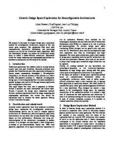
Fig. 1. Parallelism levels in traditional embedded processors and data-parallel embedded stream processors
2 Background 2.1 Stream processors Special-purpose processors for wireless communications perform well because of the abundant parallelism and regular communication patterns within physical layer processing. These processors efficiently exploit these characteristics to keep thousands of arithmetic units busy without requiring many expensive global communication and storage resources. The bulk of the parallelism in wireless processing can be exploited as data parallelism, as identical operations are performed repeatedly on incoming data elements. An embedded stream processor can also efficiently exploit this kind of data parallelism. Figure 1 shows the different parallelism levels exploited in such an embedded processor. Traditional programmable embedded processors such as DSPs exploit instruction level parallelism (ILP) and subword parallelism (SubP) [4]. Embedded stream processors exploit data parallelism (DP), in addition to ILP and subword parallelism, enabling high performance programmable architectures with hundreds of ALUs. All clusters in the data-parallel embedded processor perform the same operations on different sets of data. The compiled application code is loaded into the micro-controller from a host processor (not shown) during run-time. The micro-controller then schedules the cluster operations to be performed on the data. The Imagine stream processor, developed at Stanford, is an example of such an embedded stream processor [1]. We use this architecture and its simulator to evaluate the design methodology presented in this paper. A stream processor simulator based on the Imagine stream pro3
cessor is available for public distribution from Stanford. The Imagine simulator is programmed in a high-level language and allows the programmer to modify the machine description features such as number and type of functional units and their latency. The cycle-accurate simulator and retargetable compiler also gives detailed insights into the ALU utilization, memory stalls, and execution time of the algorithms. A power consumption and VLSI scaling model is also available to give a complete picture of the power and performance of the resulting architecture. 2.2 Application domain Wireless communications provide a great example for exploring embedded processor configurations, requiring high performance while minimizing on metrics such as power. Over the last few years, the data rates for wireless systems have increased rapidly from Kbps for voice applications to Mbps for multimedia applications. Moreover, sophisticated signal processing algorithms are now being used to reliably process a bit of information received over the wireless channel. The increase in the amount of bits needed to be processed in unit time along with the increase in computational complexity now requires the support of hundreds of arithmetic units for real-time processing. The need for flexibility in wireless systems have also increased due to the need to support different environments and wireless standards and allow algorithm designers to quickly design and implement algorithms on these systems. This paper addresses the challenges in the design of an embedded processor that can provide large number of arithmetic units to meet real-time requirements and provides flexibility by being fully programmable, in the sense that there is no hardware customization provided for any application such as co-processors for decoding in DSPs [5]. We choose a wireless base-station as a design workload that requires 24 billion computations per second [6], employing sophisticated signal processing algorithms such as multiuser estimation, multiuser detection and Viterbi decoding and providing 128 Kbps data rate per user for 32 users in the base-station. 2.3 Related work Design space exploration for embedded systems have traditionally been in the low power, heterogeneous system domain [7], where the focus has been to find the best partition of algorithms among the different types of hardware used in the design. On the other hand, design space exploration for power minimization or attaining real-time has not been a focus for high performance programmable processors supporting � � ’s of functional units. The combination of programmable solutions for embedded systems along with the need for high performance with � � ’s of arithmetic units presents new design challenges for the embedded system designer. Design space exploration has been studied for VLIW-based embedded processors [8, 9] for performance and power. These techniques directly relate to a design exploration for a single cluster stream processor. However, exploring the number of clusters in the design adds an additional dimension to the search space and it is not clear as to how to partition the arithmetic units into clusters and the number of arithmetic units to be put within each cluster. Design space exploration has also been studied for on-chip MIMD multiprocessors based on linear programming 4
methods [10] to find the right number of processors (clusters) for performance and energy constraints, assuming a fixed configuration for parameters within a cluster. The design space exploration using these techniques for stream processors need a more exhaustive and complex search for simultaneous optimization for the number and types of arithmetic units within a cluster. The tradeoffs between exploiting ILP within a cluster and across clusters increases the complexity of the design exploration. We show that the explicit use of data parallelism across clusters in a stream processor can be exploited to provide a simpler method to find the right number of clusters and the number and types of arithmetic units within a cluster for stream processors. The base Imagine stream processor [1] was designed by running experiments with the media processing algorithms and picking the solution that was thought reasonable to build and that yielded the best performance and utilization. Our design methodology tool seeks to formalize an approach to designing stream processors in the future, optimizing on metrics such as power.
3 Design exploration framework We present a design space exploration tool heuristic based on two important observations. Observation 1 Signal processing workloads are compute-bound and their performance can be predicted at compile-time. The execution time of signal processing workloads is fairly predictable at compile time due to the static nature of signal processing workloads. Figure 2 shows the execution time for a workload being composed of two parts: computations ���� � �� , and stalls ��
. The memory stalls are difficult to predict at compile time as the exact area of overlap between memory operations and computations is determined only at run-time. The microcontroller stalls depends on the data bandwidth required by the arithmetic units in the clusters and varies with the algorithms, the number of clusters and the availability of the data in internal memory. Some parts of the memory and microcontroller stalls are constant due to internal memory size limitations or bank conflicts and do not change with the computations. The processor clock frequency needed to attain real-time is directly proportional to the execution time and we will use frequency instead of time in the analysis in the rest of the paper. As the computation time decreases due to addition of arithmetic units (since we are compute-bound), some of the memory stalls start getting exposed and are thus, variable with ���� � � �� . The real-time frequency needed to account for constant memory stalls that do not change with computations is denoted by ��� �� . The worst-case memory stalls, �� �� occurs when the entire ILP, DP and SubP are exploited in the processor, which changes the problem from compute bound to memory bound. Hence, the memory stall time is bounded by � �� �� and �� �� .
� � ��� � � �� � � ��
� � � � � ��� �� � � ��
� �� ��
5
(1)
Microcontroller stalls
tstall
Exposed memory stalls
t mem
Hidden memory stalls
Total Execution Time (cycles) t compute
Computations
Fig. 2. Breakdown of the real-time frequency (execution time) of a workload
Definition 1 Data Parallelism (DP) can be defined as the number of data elements that require the exact same operations to be performed in an algorithm and is architecture-independent. In this paper, we define a new term, cluster data parallelism (CDP � DP), as the parallelism available in the data after exploiting SubP and ILP. Thus, cluster data parallelism is the maximum DP that can be exploited across clusters without significant decrease in ILP or SubP. ILP exploitation within a cluster is limited due to finite resources within a cluster such as finite register sizes, inter-cluster communication bottlenecks and finite number of input read and output write ports. Increasing some of the resources such as register file sizes are less expensive than adding an extra inter-cluster communication network [11], which can cause a significant impact on the chip wiring layout and power consumption. Any one of these bottlenecks is sufficient to restrict the ILP. Also, exploiting ILP across basic blocks in applications with multiple loops is limited due to the compiler [3]. Signal processing algorithms tend to have significant amounts of data parallelism [1, 6, 11, 12]. Hence, DP is available even after loop unrolling due to finite resources, and can be used for setting the number of clusters as CDP. Observation 2 Due to limited resources within a cluster, not all DP can be exploited as ILP in stream processors via loop unrolling. The unutilized DP can be exploited across clusters as CDP. This observation allows us set the clusters according to the CDP and set the arithmetic units within the clusters based on ILP and SubP, decoupling the problem of a joint exploration of clusters and arithmetic units within a cluster into independent problems. This provides a drastic reduction in the exploration space and in programming effort for various cluster configurations. The observation is best demonstrated by an example of the Viterbi decoding algorithm used in 6
5
Rate 1/2 Viterbi decoding for 32 users
10
Execution time (cycles)
Constraint length = 9 Constraint length = 7 Constraint length = 5
4
10
3
10 0 10
1
10
2
10
Number of clusters
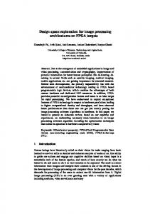
Fig. 3. Viterbi decoding performance for varying constraint lengths and clusters, assuming a cluster has 3 adders and 3 multipliers
wireless communication systems. Figure 3 shows the performance of Viterbi decoding with increasing clusters in the processor for � users done sequentially assuming a constant cluster configuration of adders and multipliers in a cluster. The data parallelism in Viterbi decoding is proportional to the constraint length, � , which is related to the strength of the error control code. A constraint length � Viterbi decoder has �� � � � �� states, and hence has DP of � �� , and can use 8-bit precision to pack 4 states in one cluster (SubP ), reducing the CDP to �� � � . Hence, increasing the number of clusters beyond � does not provide performance benefits. However, as the clusters reduce from � to for � � , we can see an almost linear relationship between clusters and execution time, showing again that the ILP and SubP being exploited can be approximated as independent of the CDP. Ideally, the CDP should be automatically determined by the compiler after it automates loop unrolling for increasing ILP and exploits SubP. Since the compiler does not automate loop unrolling, the burden of deciding the CDP is currently left to the programmer. The deviation of the performance curve with clusters from a slope of � represents the variation of ILP with CDP.
3.1 Design exploration framework We base our design exploration framework on the two assumptions that were discussed in the previous section. Let the workload , consist of algorithm kernels executed sequentially on the data-parallel embedded processor; given by � , �� , ... , �� . Let the functional units in � the embedded processor be assumed to be solely adders and multipliers, for the��purpose of �� � � � � � � � � �� this�� analysis. Let the respective execution time of the kernels be , � , ..., � � � �� �� � � , where ( , , ) be the number of adders per cluster, the number of multipliers per � cluster and the number of clusters respectively. Let the cluster data parallelism in each of these 7
kernels be defined as
� � �
,
� �
� , � � �,
� �
�.
The design phase consists of a worst-case workload that needs to be designed to meet realtime constraints in a programmable architecture. The exploration tool then searches for the �� � � �� best ( � ) configuration that minimizes the power consumption of the processor for that workload. Once the chip is designed, the architecture can run the workload as well as other �� � � �� application workloads by dynamically adapting ( � ) parameters to match that of the application [13]. Thus, the solution provides possibilities for using this designed architecture for investigating run-time variations in the workload and adapting to the variations. Our design goal � � � is to find ( , , , � ), such that the power � � �� �� �� � is minimized. �
� �� �� ��
� � �� � � � � � � �� � � � �� � �� �� ��
(2)
� �� � � � � �
�� � � � � �
where is the loading capacitance, is the supply voltage and � is the clock frequency needed to meet real-time requirements. The model for the capacitance is derived from the Imagine stream processor implementation and is presented in the appendix. Now, to achieve the real-time frequency � , the processor voltage also needs to be set. The voltage is dependent on the clock frequency needed in the processor. � �
where
�
�
�� �
(3)
is the threshold voltage [14]. Hence, from equations (2) and (3), we get
�
� �� ��
� � �� � � � � �
� � �� �� � �� ��
(4)
The design space exploration tool shown in the next section optimizes equation (4) to find the number and organization of the arithmetic units that minimizes the power consumption. 3.2 Sensitivity analysis As transistors have gone towards the deep-submicron regime, the transistors are getting shorter and saturating at lower drain-to-source voltages [15]. The relationship between the drain current and the gate-to-source voltage has gone down from quadratic to linear [16]. This effect is also known as velocity saturation due to short channel effects. Velocity saturation thus affects the delay variation in the transistor with voltage from being quadratic as shown in equation (3) to being linear with voltage. Hence, the relationship of power with frequency is changing from being cubic to being quadratic with frequency. Decreasing the threshold voltage helps but the trends still continue as the threshold voltage cannot be decreased at the same rate as the drain-to-source voltage [15]. The actual 8
value of the relationship between power and frequency is very much technology dependent. Hence, to analyze the sensitivity of the design to the technology, we assume, � � �� �� �
�
�
� �� ��
� ��� �
� �
�
� � �� � � � ��
�� ��
� � �
�
�
(5) (6) (7)
� � � �� �� �
where � is the velocity saturation model for the transistor, with � representing full velocity saturation. This model thus allows the designer to set � according to the technology, and explore the sensitivity of the design to � . Similarly, functional units in an actual physical realization can have different power consumption values than those used in a power model. If we assume two types of functional units such as adders and multipliers in the design, we need to model the power consumption of one relative to the other to make the values used independent of the technologies and actual implementations. Adder and multiplier power consumptions are linear and quadratic multiplier with the bit-width � respectively [17]. � -bit adder designs and � � � multiplier designs can have relative power ratios varying between � � % after normalizing their bit-widths to � [18]. Hence, for our paper, using equally aggressive � -bit adders and � � � multipliers, we will assume variations in adder power to be between � �� and � � of the multiplier power. As will be seen later, this variation is not critical as the additional register files and the intra-cluster communication network that gets added with the functional units dominate the power consumption instead of the functional units by themselves. � � � ��
�
� � � � �� � � �
�
� � � ��
�� � �� � �
� �
� � � � �� � � �
� ��� �
� � ��
� � �
��
�
(8) (9) (10)
The organization of the stream processor provides a bandwidth hierarchy, which allows prefetching of data and mitigates memory stalls in the stream processor [12, 19]. Memory stalls have been shown to account for � � � % of the total execution time in media processing workloads [19] and �� % of the execution time in wireless communication workloads [13]. Stalls are caused in stream processors due to waits for memory transfers (both external memory and microcontroller stalls), inefficiencies in software pipelining of the code, and time taken to dispatch microcontroller code from the host processor to the microcontroller [19]. However, with more effort on developing the compiler tools and programming using techniques such as stripmining [19], these memory stalls can be mitigated. In order to model memory stalls and observe the sensitivity of the design to the stalls, we model the worst-case stall �� �� to be �� % of the workload at the minimum clock frequency that is needed for real-time � �� � where the entire available ILP, DP and SubP are exploited. We then back off the stalls with increase in � by a parameter . 9
Hence, we will model variations in between � and tools to the stalls. Hence, from equation (1),
� ��
� ��
�
�
� �� �
�
�
�� ��
�
�
� ��� �
�
�
� �
�
�� �
to explore the sensitivity of the design
(11) (12)
represents the no-stall case and � represents the worst-case memory stall �� �� . The minimum real-time frequency, �� � , is computed during the design exploration. There are other parameters in an embedded stream processor that can affect performance and need exploration such as the number of registers and pipelining depth of arithmetic units [2, 8, 9]. These parameters affect the ILP for a cluster and hence, indirectly affect the CDP. Although an exploration for these parameters will affect the actual choice for the design, the design exploration methodology does not change as we decouple ILP and DP in our design exploration. In �� order to stress � � � �� � � for the design methodology and our contributions, we focus on the exploration of � � �� � �� � � � � � � � have power minimization and their sensitivity to three parameters: � . Once been decided, other parameters can be decided based on this configuration.
4 Design space exploration We start the design exploration with an over-provisioned hypothetical architecture, having infinite clusters and infinite arithmetic units within each cluster. This hypothetical architecture exploits ILP, SubP and DP to the maximum to provide the minimum real-time frequency possible in the embedded stream processor. We then curtail the ALUs in each cluster and the number of clusters to decrease the capacitance to a point until which there is no loss in performance with the decrease in the number and organization of the arithmetic units. At this point, further decrease in either clusters or ALUs within a cluster increases the clock frequency and hence, this provides the revised starting point for exploring the trade-offs between frequency and capacitance in equation (7). The observations presented in the previous section decouple the joint exploration of clusters and arithmetic units within a cluster to independent explorations, providing a drastic reduction in the exploration space and in programming effort for exploring different cluster configurations. Thus, the exploration of ILP and SubP to set the arithmetic units within a cluster and the CDP to set the number of clusters in the embedded stream processor can be done independently. However, it has been observed in [11, 12] that it is more efficient and lower power to exploit DP across clusters than within a cluster. Hence, our design tool heuristic explores the cluster space first to maximize the number of clusters based on the CDP before exploring the arithmetic units within a cluster. 10
4.1 Setting the number of clusters To find the number of clusters needed, we compile all kernels at their maximum data parallelism (CDP) levels, assuming a sufficiently large number of adders and multipliers per cluster, large enough to exploit the� maximum ILP available in the cluster. i.e. we run kernel with � �� �� � �� ( � � � � � ) where � � � � are a sufficiently large enough number of adders and multipliers per cluster to exploit the available ILP in all kernels. The compile-time execution for kernel is given by � �� � � � �� � � � �� �� � � . Hence, the real-time frequency � � � �� �� �
�� � � � ��
for c clusters is
(MHz) Real-time target(Mbps) * Execution time per bit(a,m,c) � �� � � � � �� � � �� � Real-time target * Execution time per bit( � � � � � ) �
� � � � � �� � � � �� � � ��
�
Real-time target �
� ��
�
�
�
�
� � � � � �� � � � �� �� � �
(13) (14) (15)
�
Equation (15) reduces the frequency by half with cluster doubling based on the observation of linear benefits of frequency with clusters within the CDP range. It also shows that if the number of clusters chosen are greater than the available CDP, then there is no reduction in execution time. The � ��
term accounts for stalls in the execution time that are not predicted at compiletime, and is computed using equations (14) and (1). The number of clusters that minimizes the power consumption is given by �
� � � � � �� � � � �� �� � � ��
�� � �� � � � �� � � � � � � � � � �� � � � �� � � ��
(16)
Thus, by computing � � � � � �� � � � �� ��� � at compile time and plotting this function for the desired range of clusters and for varying , the number of clusters that will minimize the power consumption is determined.�This function essentially says that if we double the number of clusters in the processor and if , the frequency should drop by at least �� �� % of the original frequency for the architecture to be lower power than the original cluster configuration. The reliability of the chosen cluster solution can be decided by the difference between the solutions � provided by exploring sensitivity to . The choice of clusters is independent of � as it gets factored out in the minimization of equation (16).
4.2 Setting the number of functional units per cluster �
Once the number of clusters is set, the ILP vs. clock frequency trade-off now needs to be evaluated for setting the number of arithmetic units within each cluster. Hence, we vary the � � � �� �� � number of adders and multipliers from to � � � � to find the trade-off point that minimizes the power consumption of the processor. Since the re-targetable compiler can handle varying arithmetic units without any changes in the application software code, an exhaustive 11
Parameter
Min
Max
CDP range
�
� ��
�
�
�
�
�
� �� �
�
Table 1 Design parameters for architecture exploration and wireless system workload
compile-time search can be now done to set the right number of adders and multipliers that meet real-time with minimum power consumption. The power minimization is now done using �
�� ��
� � �� �� �� �
� � �� � � � � �
�� ��
� � � �� �� �
(17)
�� � � �
and exploring exhaustively. The design tool also spits out information about the arithmetic unit efficiencies based on the schedule. It can be shown (not shown due to space considerations) that this power minimization is related to maximization of the ALU utilization, providing us with insights about the relation between power minimization and the ALU utilization. The � choice of arithmetic units inside a cluster is dependent on � , and .
5 Results For evaluation of the design exploration methodology, the design concept was applied for designing a � base-station embedded processor that meets real-time requirements. For the purposes of this paper, we consider a � -user base-station with � Kbps/user (coded), employing multiuser channel estimation, multiuser detection and Viterbi decoding [6, 13]. This was considered to be the worst-case workload that the processor needed to support in the design. The design boundary conditions used for the workload are shown in Table 1. Ideally, the CDP range should be decided by the exploration tool with the help of the compiler. The compiler should automatically exploit all the available ILP (using loop unrolling) and SubP and set the remaining DP as CDP. In the absence of the compiler’s ability to automate this process, the CDP has been set manually after exploring different amounts of loop unrolling and finding out the changes in ILP. At least clusters are needed to make up for the loss in performance due to vectorization of the algorithms and there is no benefit in performance after � � clusters as that is the maximum CDP available. Similarly, the adders and multipliers are varied between and � for the adder and and for the multiplier as we have seen ILP saturating above these configuration levels with no benefits in performance. These ranges will be confirmed in the design exploration process. Table 2 shows the break-up of the workload computations for attaining the lowest real-time � � � � � �� � � frequency that is obtained at compile-time using equation (15) and replacing � by � . 12
Algorithm
Estimation
Detection
Decoding
Kernel
CDP
Cycles
Correlation update
�
Matrix mul
�
�� ���
Iteration
�
�� �
�
transpose
� ��
��
� �
�
�
��
Matrix mul L
�
�
Matrix mul C
�
��
Matched filter
�
� ���
Interference Cancellation
�
�� �� �
Packing
�� �
Re-packing
�
Initialization
�
Add-Compare-Select
�
Decoding output
�
� � � �
MHz needed
�
�� �� � �
�
� �
���
� �
� �
�
�
��� �
��
��
�� �
�
Min real-time frequency � � � � � �� � �� � �
� �
�
Mathematically required ALU op count
�
�
�
GOPs
Table 2 Real-time frequency needed for a wireless base-station providing �� � Kbps/user for � users
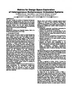
We can see that the CDP varies in the algorithms between � and � � , justifying the range for CDP exploration in Table 1. We also note that since more than � � % of the real-time frequency is needed by kernels that require � and � clusters, there is little advantage in exploring higher number of clusters. The minimum real-time frequency needed �� � is � MHz, where the available ILP, DP and SubP are exploited to the maximum degree in the processor. Figure 4 shows the real-time frequency of the workload with increasing clusters as is varied, using equations (15). Since the minimum CDP is � , the execution time decreases linearly until � and then no longer provides a linear decrease as seen from equation (15). Further increasing the clusters above � clusters has almost no effect on the execution time as the algorithms using the higher CDP take less than % of the workload time, as shown in Table 2. Figure 5 shows the variation of the normalized power with increasing clusters as clock frequency decreases to achieve real-time execution of the workload. This is obtained from equation (16). The thick lines show the ideal, no stall case of and the thin lines show the variation as decreases to � . The figure shows that as the number of clusters increase, the power consumption comes down drastically up to � � � less than the original power consumption as the number of clusters reaches � clusters from a cluster architecture. After � clusters, the increase in capacitance outweighs the small performance benefits, increasing the power consumption. Sec13
4
10
Frequency (MHz)
β=0 β = 0.5 β=1
3
10
2
10 0 10
1
2
10
3
10
10
Clusters
Fig. 4. Variation of real-time frequency with increasing clusters 0
Normalized Power
10
−1
10
−2
10
2
Power ∝ f 2.5 Power ∝ f 3 Power ∝ f
−3
10
0
1
10
2
10
10
3
10
Clusters
Fig. 5. Minimum power point with increasing clusters and variations in
and �
ondly, the figure shows that the design choice for clusters is actually independent of the value � of and as all variations show the same design solution. �
�
Cluster choice : � clusters � ( , � , )
Once the number of clusters are set, a similar exploration is done within a cluster to choose the number of adders and multipliers within a cluster and minimizing power using equation (17). Figure 6 shows the variation of the real-time frequency with increasing adders and multipliers in the workload. The utilization of the adders and multipliers are obtained� from the compile-time � � analysis of the workload using the design tool and are represented as � � respectively. The figure shows that after the ( adder, multiplier) point there is very little benefit in performance due to the addition of more adders or multipliers, which implies that, that is the point where 14
(78,18)
(78,27) 1200
(50,31)
(78,45)
(39,28)
(65,46) (51,42) (67,62)
600
(55,62)
400 1 2
(43,56)
(42,37)
(36,54)
(33,34) 2
3
ip lie rs
800
(32,28)
ul t
1000
(64,31)
3 4
#Adders
5
1
#M
Rea l-T im e Freq ue nc y (in MHz) with AL U utilizatio n(+,*)
Initial (5,3,64) (541 MHz)
Final (3,1,64) (567 MHz)
Fig. 6. Real-time frequency varying adders and multipliers for � � � � , �� � � �variation � � with �� � �� � , refining on the � � � solution
� � �� �, �
= 1,
the entire ILP is exploited and adding more units does not produce any benefits. However, the ( � adder, multiplier) point has a higher functional unit utilization. Hence, one could expect one of these configurations to� be� � a low power solution as well. The actual low power point � � � � �� , = 1,
depends on the variation of in the design. For the case of , the �� � � � � � � � � �
� obtains the minimum power as computed from equation (17). Figure 7 shows the power minimization sensitivity of the arithmetic units within each cluster � � with , and � . The columns in Figure 7 represent the variations in . The first 3 rows show the sensitivity of the design to variations in memory stalls , while the last row shows the sensitivity of the design to � . By looking at the array of subplots, we make the following observations. First, �� � � � � � there are only 2� configurations of that the exploration yields after a sensitivity analysis: � � � � � � � � � � and � . Second, the design is most sensitive to variations in . We can see that � � � � � �
� always has the � � configuration and always has the (3,1,64) configuration. � This is expected as variations in affect the power minimization in the exponent. We can see � � � � � � � � � have among the highest ALU utilizations and from Figure 7 that the � � and this shows the correlation between power minimization and ALU utilization for our design. Third, we see that the design is also sensitive to memory stalls . We can see that for � , � � � � which represents the worst-case memory stall, the design choice is � � and it changes to � � � � � as increases. Thus, memory stalls affect the design in a manner similar to reduction � in . Finally, we see that from the last row that the design is relatively insensitive to � variations. This is because, the register files and associated intra-cluster communication network that get added with increase in arithmetic units dominate the power consumption, taking � � � � � % of the cluster power for the configurations studied. The cluster power, on the other hand, take between 15
�� � �
% of the total chip power for the designs explored.
α = 0.01, β = 0, p = 2 Min = (2,1,64)
0 3 2 1 1
Multipliers
3
2
4
5
2 1.5 1 1
Multipliers
Adders
α = 0.01, β = 0.5, p = 2 Min = (2,1,64)
0.5
0 3 2 1.5 1 1
3
2
Multipliers
2.5 2 1.5 1 1
Multipliers
α = 0.01, β = 0.5, p = 2.5 Min = (3,1,64)
4
5
2 1.5 1 1
3
2
Multipliers
4
5
2.5 2 1.5 1 1
Min = (3,1,64)
0.5
1 1
Multipliers
3
2
5
2 1.5 1 1
Multipliers
α = 0.1, β = 1, p = 2
Min = (2,1,64)
0.5
0 3
3
2
4
5
2 1.5 1 1
2
Multipliers
3
4
5
1.5 1 1
Multipliers
α = 0.1, β = 1, p = 2.5 Min = (3,1,64)
(a) p = 2
3
2
4
5
Adders
α = 0.1, β = 1, p = 3
Min = (3,1,64)
1
0.5
0.5
0 3 2.5 2 1.5 1 1
Adders
2.5 2
0 3 2.5
0.5
Adders
1 Power
1
Min = (3,1,64)
0 3 2.5
Adders
5
Adders
1
Power
1.5
4
4
α = 0.01, β = 1, p = 3
0 3 2.5
3
2
Multipliers
Power
Power
0 3 2
Min = (3,1,64)
0.5
Adders
1
0.5
5
Adders
α = 0.01, β = 1, p = 2.5
Min = (2,1,64)
1
4
0 3 2.5
Adders
3
2
α = 0.01, β = 0.5, p = 3
1
0.5
α = 0.01, β = 1, p = 2
Power
5
0 3 2.5
Power
3
2
4
Adders
1 Power
1
0.5
0 3 2.5
Power
1.5
Power
0.5
0 3 2.5
Min = (3,1,64)
1 Power
0.5
α = 0.01, β = 0, p = 3
Min = (2,1,64)
1 Power
1 Power
α = 0.01, β = 0, p = 2.5
Multipliers
3
2
4
5
2.5 2 1.5 1 1
Adders
(b) p = 2.5
Fig. 7. Sensitivity of power minimization to ,
2
Multipliers
3
4
5
Adders
(c) p = 3 and � for � � clusters
5.1 Cluster utilization The design exploration for the workload shows in Figure 5 that the � cluster architecture to be � � lower power than the � cluster case, due to the cubic dependency of power on frequency. However, the � cluster architecture attains cluster utilization of only � % in cluster numbers � � as opposed to � � % utilization in a � cluster architecture (or in the first � clusters of a � cluster architecture). Thus, it is interesting to note that a � cluster architecture which will 16
never obtain �� % cluster utilization for the workload will have a lower power consumption than a � cluster architecture with a � � % cluster utilization, merely due to the ability to lower the clock frequency, which balances out the increase in capacitance. When the CDP during execution falls below � (which occurs for algorithms having CDP = � in the workload), clusters � � remain unused for 46% of the time as there is not enough CDP in those algorithms to utilize those clusters. It is clear from the plot that further power savings can be obtained by dynamically turning off entire clusters when the CDP falls below � clusters during execution. Since clusters in the � cluster architecture consume � � � � % of the total power consumption of the chip, turning off the � unused clusters can reduce the power consumption by up to � % during run-time. A multiplexer network between the internal memory and clusters can be used to provide this dynamic adaptation for power savings by turning off unused clusters [13] using power-gating. Further power can also be saved by turning off unused functional units when workloads having different ALU utilizations are getting executed. The benefits due to this adaptation are limited as the ALUs consume only � � � % of the power consumption in a � cluster architecture configuration.
5.2 Verifications with detailed simulations �
The design exploration tool gave two configurations as the output for variations in , � and . � �
Design Design
�� � � � � �
�� � � � � �
� � �
�
� � � �
�
� � � �
�
: �� � � � �� �� � � � � � �� � �� � �� � � � � � � � � � � � � � � � :
� � � � � � � �
Table 3 provides the design verification of the tool (T) with a cycle-accurate simulation (S) using the Imagine stream processor simulator that can produce details on the execution time, such as the computation time, memory stalls and microcontroller stalls. From the Table, we can observe the following things. First, the design tool models the compute part of the workload very realistically. The relatively small errors are due to the assumption of ILP being independent of CDP and due to the prologue and epilogue effects of loops in the code that were ignored. Second, we can see that both the design configurations are very close in their� power consumptions, � � � � � � � � configuration being only � � with the % different than the � � configuration. We compare this design tool by a carefully chosen human analysis for a configuration, which we had performed earlier [6, 13]. We had observed that most operations in the workload were additions and multiplications and the mathematical op count for them were approximately the �� � � � � � � same [6]. Hence, we had chosen an = configuration as a good choice for the design. Secondly, due to the fact that cluster configurations above � clusters never achieve more than � % utilizations in our workload, made us choose that configuration as the choice of clusters and � � � � � � � � we made a choice of � as our architecture for exploration in [13]. The reason � � � � � � and � are chosen by the design tool is that the adder, multiplier ratio is skewed in an actual implementation due to extraneous operations that occur in an algorithm to processor mapping such as loop increments, dependencies between the operations and number and types of arithmetic units. Secondly, the � additional clusters in the � cluster configuration provide 17
�
Choice
�� � � � � �
Design �
� � � �� � � �
� � � �� � �
� � �
�
�
Exposed
Total
Real-time
time
stalls
stalls
time
frequency
(cycles)
(cycles)
(cycles)
(cycles)
(MHz)
�
�� ���
��
�� � �
��
T
� ��
�� ���
�����
� ��� ��
��
T
�
�� ���
�
�� � ��
�� �
��� �
��
�� � �
�
�
� � ��
���
T
�
� � � � ��
��
� � ��
T
� ��
� � � � ��
�����
�� � � �
�
T
�
� � � � ��
�
� � � � ��
��
� �� � � �
� � �
� � �� �
���
� ��
���
� � �� � �
��
�� ���
�� �
�
S Human
C
T
S Design � �
Compute
�
��
� � � �
�� � ��
T
�
� � �� � �
��
T
� ��
� � �� � �
�����
T
�
� � �� � �
�
S
��
�
�
� ��� �
��� � �
�
Relative Power
�� � � � � �
Consumption � �
� � ��
�
�
�
�
� �� �
� � ��
� �� �
� �� �
� � ��
� �� �
��
�
� ���
�� �
Table 3 Verification of design tool output (T) with a detailed cycle-accurate simulation (S)
% performance improvement and meets the criteria for increasing a benefit of �more than �� � clusters for � and . It tells us that even an inefficient implementation with lower cluster utilization can be lower power if it reduces the clock frequency by the right amount. Thus, we see that the design tool provides us with lower power configurations than a carefully chosen human configuration and beats it by a factor of �� � � � �.
6 Conclusions Trade-offs exist between the choice and arrangement of arithmetic units and clock frequency of embedded stream processors to minimize metrics such as power consumption. We have developed a design exploration tool that explores this trade-off and presents a heuristic that minimizes the power consumption in the (functional units, clusters, frequency) design space. Our design methodology relates the instruction level parallelism, subword parallelism and data parallelism to the organization of the functional units in an embedded stream processor. We base our heuristic on the assumptions of the compute-intensive nature of the workloads, independence of ILP with cluster variations over a range of clusters, and the fact that cluster variations have a more significant impact on the power than variations in arithmetic units within a cluster. This heuristic enables us to decouple the exploration phase of clusters and arithmetic units per cluster into independent explorations, providing a drastic reduction in the search space and decreasing 18
�
programming effort. The design exploration tool also provides insights into the functional unit utilization of the processor and provides a quick lower bound estimate of the processor performance and power. Our design exploration tool can be applied to all embedded stream processor design applications in signal and media processing for meeting real-time requirements while minimizing power consumption. With improvements in compilers for embedded stream processors, the design exploration tool heuristic can also be �� improved by incorporating techniques such as integer linear programming � � � �� � for jointly exploring � as well as exploring other processor parameters such as register file sizes and pipeline depths of arithmetic units. Also, once the design is done for the worst case, techniques such as voltage-frequency scaling, turning off unused clusters and functional units [13] can be used to adapt such data-parallel embedded processors to provide further power efficiency against run-time variations in the workload.
References [1] U. J. Kapasi, S. Rixner, W. J. Dally, B. Khailany, J. H. Ahn, P. Mattson, and J. D. Owens. Programmable stream processors. IEEE Computer, 36(8):54–62, August 2003. [2] D. Marculescu and A. Iyer. Application-driven processor design exploration for power-performance trade-off analysis. In IEEE International Conference on Computer-Aided Design (ICCAD), pages 306–313, San Jose, CA, November 2001. [3] P. Mattson, W. J. Dally, S. Rixner, U. J. Kapasi, and J. D. Owens. Communication Scheduling. In 9th international conference on Architectural support for programming languages and operating systems(ASPLOS), volume 35, pages 82–92, Cambridge, MA, November 2000. [4] R. Leupers. Instruction Scheduling for clustered VLIW DSPs. In International Conference on Parallel Architectures and Compilation Techniques (PACT’00) , pages 291–300, Philadelphia, PA, October 2000. [5] S. Agarwala et al. A 600 MHz VLIW DSP. In IEEE International Solid-State Circuits Conference, volume 1, pages 56–57, San Fransisco, CA, February 2002. [6] S. Rajagopal, S. Rixner, and J. R. Cavallaro. A programmable baseband processor design for software defined radios. In IEEE International Midwest Symposium on Circuits and Systems, volume 3, pages 413–416, Tulsa, OK, August 2002. [7] H. Blume, H. Hubert, H. T. Feldkamper, and T. G. Noll. Model-based exploration of the design space for heterogeneous systems on chip. In IEEE International Conference on Application-specific Systems, Architectures and Processors, pages 29–40, San Jose, CA, July 2002. [8] V. S. Lapinskii, M. F. Jacome, and G. A. de Veciana. Application-specific clustered VLIW datapaths: Early exploration on a parameterized design space. IEEE Transactions on Computer-Aided Design of Integrated Circuits and Systems, 21(8):889–903, August 2002. [9] J. Kin, C. Lee, W. H. Mangione-Smith, and M. Potkonjak. Power efficient mediaprocessors: Design space exploration. In ACM/IEEE Design Automation Conference, pages 321–326, New Orleans, LA, June 1999.
19
[10] I. Kadayif, M. Kandemir, and U. Sezer. An integer linear programming based approach for parallelizing applications in on-chip multiprocessors. In ACM/IEEE Design Automation Conference, pages 703–708, New Orleans, LA, June 2002. [11] B. Khailany, W. J. Dally, S. Rixner, U. J. Kapasi, J. D. Owens, and B. Towles. Exploring the VLSI scalability of stream processors. In International Conference on High Performance Computer Architecture (HPCA-2003), pages 153–164, Anaheim, CA, February 2003. [12] S. Rixner, W. Dally, U. Kapasi, B. Khailany, A. Lopez-Lagunas, P. Mattson, and J. Owens. A bandwidth-efficient architecture for media processing. In 31st Annual International Symposium on Microarchitecture, pages 3–13, Dallas, TX, November 1998. [13] S. Rajagopal, S. Rixner, and J. R. Cavallaro. Reconfigurable stream processors for wireless basestations. Rice University Technical Report TREE0305, October 2003. [14] A. P. Chandrakasan, S. Sheng, and R. W. Brodersen. Low Power CMOS Digital Design. IEEE Journal of Solid-State Circuits, 27(4):119–123, 1992. [15] J. A. Butts and G. S. Sohi. A static power model for architects. In 33rd Annual International Symposium on Microarchitecture (Micro-33), pages 191–201, Monterey, CA, December 2000. [16] M. M. Khellah and M. I. Elmasry. Power minimization of high-performance submicron CMOS circuits using a dual- � � dual- � � (DVDV)approach. In IEEE International Symposium on Low Power Electronic Design (ISLPED’99), pages 106–108, San Diego, CA, 1999. [17] A. Bogliolo, R. Corgnati, E. Macii, and M. Poncino. Parameterized RTL power models for combinational soft macros. In IEEE International Conference on Computer-Aided Design (ICCAD), pages 284–288, San Jose, CA, November 1999. [18] A. Beaumont-Smith, N. Burgess, S. Cui, and M. Liebelt. GaAs multiplier and adder designs for �� high-speed DSP applications. In � Asilomar Conference on Signals, Systems and Computers, volume 2, pages 1517–1521, Pacific Grove, CA, November 1997. [19] J. D. Owens, S. Rixner, U. J. Kapasi, P. Mattson, B. Towles, B. Serebrin, and W. J. Dally. Media processing applications on the Imagine stream processor. In IEEE International Conference on Computer Design (ICCD), pages 295–302, Freiburg, Germany, September 2002.
A
Capacitance model for embedded stream processors
To estimate the capacitance, we use the derivation for energy of a stream processor from [11], which is based on the capacitance values extracted from the Imagine stream processor fabrica� �� � � � �� in our tion. The equations in [11] have been modified to relate to the calculation of paper instead of energy in [11]. Also, the equations now consider adders and multipliers as separate arithmetic units instead of a global ALU as considered in [11]. Due to space considerations, we refer the reader to [11] for details on the capacitance model.
20