John W. Suh, Samuel B. Homans & Mark H. Yim. Telecubes: mechanical design of a module for self-reconfigurable robotics. In IEEE Int. Conf. on Robotics and ...
Designing Modular Lattice Systems with Chiral Space Groups Nicolas Brener, Faiz Ben Amar, Philippe Bidaud Universit´e Pierre et Marie Curie - Paris 6 Institut des Syst`emes Intelligents et de Robotique, CNRS FRE 2507 4 Place Jussieu, 75252 Paris Cedex 05 , France Email : {brener, amar, bidaud}@robot.jussieu.fr October 31, 2007 Abstract We propose to use the concept of chiral space groups used by the crystallography science to define and design lattice robots. Chiral space groups are of great interest because they give all possible sets of discrete displacements having a group structure and a translational symmetry. We explain the analogy between lattice robot kinematics and crystal symmetry, and identify three fundamental properties of lattice robots such as (1) discreteness (2) translational symmetry and (3) composition. Then we give the possible connectors symmetries and orientations into a chiral space group, and the possible sliding and hinge joints locations and orientations compatible with the displacements in chiral space groups. We present a framework for the design of lattice robots by assembling compatible joints and connectors into a chiral space group. Several 2D and 3D examples of design are given to illustrate the framework. Moreover, we list the symmetries of the two chiral space groups P432 and P622 because they contain the symmetries of all the 65 chiral space groups and allow to design any lattice system.
1
Introduction
A modular robotic system (MRS) is composed of multiple building blocks (i.e. mechatronic modules) having docking interfaces to connect them together. Structure and operating modes of such a system depend on the way the modules are connected together. It is possible to reconfigure the MRS topology by adding/removing one or several modules to the system, or by changing the way the modules are connected together. A reconfiguration is a sequence of connections, disconnections, and displacements of modules. Moreover, self-reconfigurable MRS can change their structure by themselves - to meet the demands of different tasks or different working environments. Such systems must be able to control the state of their connectors and move their modules around. These systems have several advantages: they are rapidly deployable, the modules can be reused and they are intrinsically versatile and robust. Among the potential applications one can mention locomotion on hazardous terrain for planetary exploration, modular manipulation, self assembly, etc... A detailed review of these systems can be found in [Brener 04]. One can distinguish chain type systems such as Polybot [Duff 01], Conro [Castano 02], and lattice systems such as I-Cube [Unsal 00], Telecube [Suh 02], Molecule [Kotay 99], Microunit [Yoshida 01], Stochastic Modular Robots [Napp 06, ], Hexagonal Metamorphic Robot [Chirikjian 96, Chiang 01, Walter 02, Walter 05]. In lattice systems, connections and disconnections occur at discrete coordinates in a virtual lattice at each step of a reconfiguration, this is not the case in chain type systems. Other systems can have both lattice and chain type configurations, such as Atron [Jorgensen 04], Molecube [Zykov 05], M-Tran [Murata 02] and Superbot [Salemi 06]. One of the main difficulty in the design of MRS concerns the definition of the module kinematics that provides a self-reconfigurable system. Lattice systems are simpler because they can take only discrete configurations but so far no method has been proposed to assist their design.
1
Figure 1: Transformation groups taxonomy. This figure shows the relation between the different transformation groups. Up: continuous groups. Down: discrete groups. Right: transformations preserving orientation. Left: transformations not preserving orientation. A box represents a unique group, and an ellipse represents a set of groups. The set of chiral space groups is underlined in bold.
This paper proposes a framework for the design of lattice systems. It relies on the discretization of the module representation on two levels. In the first one, the symmetries of the connectors are represented by point groups and in the second one the discrete configurations which can be produced on the connectors by the MRS actuators are represented by discrete displacements groups. For representing the different kinematical structures of the system we use special discrete displacement groups, the space groups provided by the crystallography science. Various methods are based on group theory, to enumerate non-isomorphic assemblies of modules [Chen 98], to perform motion planning [Pamecha 97], to automatically derive dynamical properties of several assembled modules[Fei 01], and others. These works consider different modules types, but do not answer the question ”how to design modules?”. In our approach we propose a method to design the kinematics of modules in lattice systems. First, we introduce chiral space groups. Second, we explain the analogy between crystal symmetries and modular lattice systems. Then we propose a framework for the design of lattice robots kinematics. Finally, we point out through existing and new examples, the advantages and the limitations of this method.
2
Introduction to chiral space groups
In the late 19th century Fedorov, Shoenflies and Barlow have introduced space groups to define and describe crystal symmetries. Using space groups, they determined the complete set of all possible crystallographic symmetries. A complete description of the theory on this subject Exhaustive data is available in [ITA 02]. Here we are only interested in a subset of the space groups, which are the chiral space groups also called Sohncke groups. Transformations involved in space groups are isometries, i.e transformation which preserve lengths like identity, rotation, translation, screw, glide, reflexion, inversion and rotoinversion. In chiral space groups, transformations are restricted to displacements which are isometries preserving orientation, like identity, rotation, translation and screw. Chiral space groups do not have isometries like glide, reflexion, inversion and
2
Figure 2: The figure describes the symmetry operations of the plane group p4 by geometric elements which are geometric items allowing symmetry operations to be located and oriented. 4-fold and 2-fold rotation axes are represented by squares and rhombus and correspond to rotations of respectively 90◦ and 180◦ . The arrows show the two elementary translations of the lattice. The nodes represent equivalent positions by translations, and are chosen coincident with the highest symmetry sites (on 4-fold rotation axes). The primitive unit cell, represented by a square in dotted lines, is a surface which tiles the plane by using only the translation symmetries, and has its vertices on nodes. The asymmetric cell represented by a dashed square tiles the plane by using all the symmetry operations. Any 90 degrees rotation along a 4-fold axes belongs to the group, any 180 degrees rotation along a 2-fold axis belongs to the group, any translation between two nodes belongs to the group. Any element of the group is one of these rotations or translations (there is no screw operation in this group), and any combination of these rotations and translations belongs to the group (it can be reduced to one rotation or one translation). The plane group p4 has two point subgroups: (1) point group 4 corresponding to the rotations along an 4-fold axis, and (2) point group 2 corresponding to the rotations along a 2-fold axis. It has also a lattice subgroup which contains the combinations of the two elementary translations. A generator of p4 can be defined by two elements: (1) one 90 degrees rotation and (2) one elementary translation orthogonal to it. Any element of p4 is a combination the two elements of the generator.
rotoinversion. To understand space groups it is useful to introduce the concepts of point groups and lattice groups. Point groups describe local symmetries, which leaves a point invariant. Lattice groups describe global symmetry with translational symmetry. Space groups combine symmetries of point groups and lattice groups to describe global symmetry having translation and other transformations. In chiral space groups, only point groups with rotations are involved. Therefore we give in the following section the definition of 3-dimensional chiral space groups, as well as point groups and lattice groups. These concepts are introduced in the Fig.2 with a 2-dimensional example.
2.1 2.1.1
Definitions and properties Chiral space group
A chiral space group (G, ∗) is an infinite set of transformations in a 3 dimensional euclidean space with the following properties: • Elements of G are displacements (identity, rotation, translation, screw), (G, ∗) is a subgroup of SE(3), • G contains 3 independent translations, • (G, ∗) has a group structure, • (G, ∗) has a discrete topology. 3
Figure 3: In (a),(b),(c),(d) the rotation axes of rotation groups 432 are shown. (a) the 3 4-fold rotation axes are parallel to the cube edges. (b) the four 3-fold rotation axes are aligned with the diagonals between the opposite vertices of the cube. (c) six 2-fold rotation axes are aligned with the diagonals of the cube faces. (d) shows all the rotation axes of the group 432. In (e) the geometric elements of group 622 are shown, there are six 2-fold rotation axes going through the opposite vertices and edges of an hexagon, and a central 6-fold rotation axis orthogonal to them.
A space group contains only discrete transformations. The crystallographic restriction theorem claims that only rotations of 0, 60, 90, 120, 180, 240, 270 or 300 degrees are compatible with discrete translations. Therefore, only such rotations will occur in space groups. The translations are combinations of the three independent elementary translations (see 2.1.4). 2.1.2
Space group type
Two space groups (G, ∗) and (H, ∗) are of same type if and only if there exists an affine transformation preserving orientation (see Fig. 1) which maps the elements of G onto the elements of H. There exists an infinite number of chiral space groups, but they are exactly 65 chiral space group types. 2.1.3
Point group, crystallographic rotation group
Point groups are discrete set of transformations which leave a point invariant. We consider only point groups which are subgroup of chiral space groups. Such point groups have only rotations (translation and screw do not leave a point invariant), we call them crystallographic rotation groups (see Fig. 1). Since these groups are subgroups of space groups the crystallographic restriction theorem applies, therefore only angles of 0, 60, 90, 120, 180, 240, 270 or 300 degrees are possible. An example is the crystallographic rotation group 432 which has 24 elements. One can represent the rotation axes of its transformations. A n-fold axis corresponds to rotations of (360/n) ∗ k degrees with 0 ≤ k < n. For example a 4-fold axis can make 0, 90, 180, 270 degrees rotations. We denote a direction vectors (x, y, z) with x, y, z ∈ {−1, 0, 1} by [x, y, z]. In an orthonormal coordinate frame, the group 432 has three 4-fold rotation axes with direction vectors [1,0,0], [0,1,0], [0,0,1], four 3-fold rotation axes with directions [1,1,1], [1,-1,-1], [-1,1,-1], [-1,-1,1], and six 2-fold rotation axes with directions [1,-1,0], [1,1,0], [0,1,-1], [0,1,1], [-1,0,1], [1,0,1]. Considering a cube, these axis directions can be viewed as, respectively, its edges, the diagonals between its opposite vertices, the diagonals of its faces, as shown in figure 3. Another example is the crystallographic rotation group 622 which has 12 elements. It has one 6-fold rotation axis and six 2-fold rotation axes perpendicular to the first one (fig 3). Thereafter, we will call the crystallographic rotation groups simply point group, because we never use point groups which are not crystallographic rotation groups. Table 2 gives the list of the 11 point group types involved 4
in the 65 chiral space groups. 2.1.4
Lattice group
A lattice group (G, ∗) is an infinite set of transformations in a 3 dimensional euclidean space with the following properties: • G contains only translations, • G contains 3 independent translations, • (G, ∗) has a group structure, • (G, ∗) has a discrete topology. In a lattice group there exists an infinite set of translations, which are equivalent to the combination of three independent elementary translations. Therefore the elements of the lattice group can be generated by combining three elementary translations which represent its translational periodicity. One can associate a parallelepiped called primitive unit cell to each lattice group in which the edges have the same lengths and orientations than the elementary translation vectors of the lattice group. The primitive unit cell can tile the space without gap. Six lattice parameters are needed to completely describe a lattice group (see [ITA 02]). The lattices can be categorized into 14 Bravais lattices depending on the lattice parameters (see [ITA 02]). 2.1.5
Orbit, site symmetry, Wyckoff site
Consider a chiral space group G, and a position e of an euclidean space E, the action of the group G on e yields an infinite set of equivalent positions called orbit. G(e) = {x ∈ E|g ∈ G, x = g(e)} Each position in the space may be (1) at the intersection of several rotation axes, (2) along individual rotation axes, or (3) elsewhere. Therefore it is possible to associate a point group to each position in the space, called site symmetry. For instance, Fig.4 shows a position and its orbit with two different site symmetries: 1. In the first case the positions are not on any symmetry axes, the site symmetry is the point group identity. 2. In the second case the positions are on 4-fold symmetry axes, the site symmetry is the point group 4. The figure shows that the number of equivalent positions per unit cell depends on their site symmetry. A set of positions X may also have an orbit G(X). For instance the group action on the set of positions X along a rotation axis yields the equivalent rotation axes G(X) into the euclidean space. In chiral space groups there exists three interesting types of sets: (1) a position at the intersection of several rotation axes, (2) the set of positions along a particular rotation axis, and (3) elsewhere. Such a set of positions corresponds to a particular site symmetry described by a point group. The orbits of such a set is called a Wyckoff site. For example the group action on the set of points along a 2-fold axis yields the equivalent 2-fold axes. The Wyckoff sites describe the equivalent locations of the site symmetries into the euclidean space associated to the space group, they give the location of symmetry invariants, such as lines along rotation axes, and points where several axes intersect. The [ITA 02] gives a description of the Wyckoff sites for each space groups. The Wyckoff sites are categorized by Wyckoff letter with higher letter matching lower symmetry. Lattice nodes are, by convention, on Wyckoff site with highest symmetry, and therefore they are on site with Wyckoff letter a.
5
Figure 4: The drawings show the 2-dimensional space group p4 with its geometric elements. Left: the cross is a position e in the euclidean space. Right: the crosses are the equivalent positions obtained by applying the transformation of p4 on the coordinate e. Top: the positions are not on rotation axes, there are 4 equivalent positions per unit cell. Bottom: the positions are on 4-fold rotation axes, there is 1 equivalent position per unit cell.
Figure 5: The four different Wyckoff sites a,b,c,d in the plane group p4
6
For instance, in the plane group p4 (Fig. 2) there are 4 different Wyckoff sites with letters a,b,c,d (depicted in Fig. 5) corresponding to 3 different site symmetries: (a) positions along the 4-fold axes at the corners of the unit cell (on the nodes) with point group 4, (b) positions along the 4-fold in the center of the unit cell (point group 4), (c) positions along the 2-fold axes in the middle of the edges of the unit cell (point group 2) and (d) positions elsewhere rotation axes (point group 1). In case (c) the 2-fold axes are equivalent because they belong to the same orbit, while the 4-fold axes in case (a) and (b) have the same site symmetry but are not equivalent (they have two different orbits). 2.1.6
Space group hierarchy
Space groups have a hierarchy. A space group G is a subgroup (respectively supergroup) of a space group H if it can be obtained by removing (resp. adding) elements of (resp. to) H. Subgroups and supergroups for each group are listed in [ITA 02]. Figure 6 shows a simplified hierarchy diagram of the 65 chiral space groups. At the bottom there is only one group called P 1 which has only translations. On the top there are four groups. One is the hexagonal P622 group with hexagonal lattice. The three others are the isometric groups P432, I432 and F432 with cubic, cubic centered and cubic face-centered lattices (see [ITA 02]). The arrows show that I432 and F432 are direct subgroups of P432, and P432 is also direct subgroup of I432 and F432. By transitivity I432 and F432 are also subgroups from each other. Therefore these three isometric groups are subgroup from each other, that means that one can be mapped to another by removing elements and applying an affine transformation preserving orientation (see 2.1.2).
Figure 6: Space groups hierarchy. Only the maximum and minimum groups are shown. On the top, the 4 maximum groups: one hexagonal and 3 isometric, on the bottom the minimum space group P1. In the middle, the remaining 60 chiral groups, whose hierarchy is not shown. The arrows show the maximum subgroups. The 3 maximum isometric groups are all subgroups of each other.
In the appendix we give a description of P432 and P622 which are at the top of the hierarchy. Any other chiral space group type can be obtained by removing elements of these groups. Instead of P432 we could take F432 or I432, but their description is more complex and P432 is in the ”middle” of I432 and F432 (see Fig.6). The space groups P622 and P432 are at the top of the chiral space group hierarchy. Nevertheless P432 has more symmetries, its point group has order 24, while P622 has order 12. Moreover P432 is ”more isotropic” than P622 because it has three equivalent orientations for its highest symmetry 4-fold rotation axes, while P622 has only one orientation for its highest symmetry 6-fold rotation axis.
2.2
Space groups in one or two dimension(s)
Space groups in one dimension are called frieze groups, and in two dimensions, plane groups or wallpaper groups. They have the same features as in 3D but less types of isometries. 7
There are 17 wallpaper groups and 7 frieze groups. The difference with space groups is that they contain respectively 2 and 1 elementary translation, instead of 3. These groups contain reflexion and glide symmetries but reflexion and glide in the plane are equivalent to rotation and screw displacement in the 3D space, therefore all these groups can be used to design lattice robots. These groups are subgroups of the chiral space groups, and therefore they are subgroups of the space groups P432 and P622. Plane groups are written with a lowercase letter while space groups are written with an uppercase one with the Hermann-Mauguin notation. An example of plane group is the plane group p4 shown in Fig.2.
3
Lattice robots and analogy with crystals
In this section we give an example of construction of a lattice robot within the space group p4 and explain the features of such systems. This is useful to define what is a lattice system. Then we give the analogy and differences between such lattice systems and crystal symmetries.
3.1
Fundamental properties of a lattice robot
We explain through an example the role of space groups in the design of lattice robot in an example. Fig.8 shows a set of equivalent coordinates (orbit) into the plane group p4. We denote G the set of displacements of p4 and X the orbit.
Figure 7: The frames represent equivalent coordinates of an orbit into the 2-dimensional space group p4. The 4-fold and 2-fold rotation axes are represented by squares and rhombus. The unit translations correspond to the edges of the unit cell drawn in dotted lines.
The figure shows also a set of 2 coordinates for black and white connectors with same position and opposite ¯ X ¯ is such that orientations. The orbit of the black connector is X, and the orbit of the white connector is X. ¯ for each x ¯ in X and for each x in X, x ¯ has the same position than x but with opposite orientations as illustrated in figure 7. By convention two connectors can be connected only if they have the same position and opposite orientations. We may use these sets of positions to construct a module with 4 configurations and two connectors shown on Fig.9. To do this we select a white coordinate x¯0 for a white connector, and four black coordinates x0..3 for the black connectors. The four black coordinates define the four configurations of the module. In this example the mechanism is implemented by two hinge joints: one has its axis aligned with a 4-fold axis of the space group, and can have two configurations of 0 degree and 90 degrees, the other one has its axis aligned with a 2-fold axis of the space group, and can have two configurations (0 and 180 degrees). The combinations of the 8
Figure 8: In (a) a connector with coordinate x corresponding to a position u and an orientation v. In (b) a connector with coordinate x0 corresponding to position u0 and orientation v 0 . In (c) two connectors with opposite coordinates x = (u, v) and x ¯ = (u, −v) are connected together.
configurations of the two hinges yield the 4 configurations of the module. The Fig.9 shows that when several modules are connected in various configurations, the black connectors have their coordinates into X, and the ¯ We denote T the lattice subgroup of G. The orbit X and X ¯ white connectors have their coordinates into X. have a translation symmetry: ∀x ∈ X, ∀t ∈ T, t(x) ∈ X ¯ ∀t ∈ T, t(¯ ¯ ∀¯ x ∈ X, x) ∈ X
Figure 9: On the left: a lattice module is built in plane group p4 by selecting a set of positions for its connectors. In this example the module has two connectors, one position is chosen for the white connector into the white orbit, and four positions are chosen for the black connector into the black orbit. Therefore the module has 4 configurations. The mechanism is implemented by two hinge joints having their axes coincident with the 4-fold and 2-fold rotation axes of the group. On the right: 3 modules are interconnected in various configurations. In each of these configurations the white connectors have their positions into the white orbit and the black connector have their positions into the black orbit. It is easy to see that for any configuration of interconnected modules the connectors have their positions into their orbit. This is due to the space group symmetry.
In this example we have three fundamental properties: 1. Discreteness: The connectors of the modules are in discrete positions into a set of coordinate called orbit. Different types of connectors can have different orbits (in the example there are a black orbit and a white orbit). 2. Translation symmetry: The orbits have a discrete translational symmetry. 3. Composition : any set of interconnected modules in any configuration have their connectors into their orbit.
9
Therefore any lattice system having these three properties can be designed by using the displacements of a space group for the joint and the corresponding orbits for the positions of the connectors. These three properties are found in lattice systems such as M-Tran [Murata 02], Molecube [Zykov 05], Molecule [Kotay 99], I-Cube [Unsal 00], Telecube [Suh 02] and Atron [Jorgensen 04]. Moreover, it is not possible to have these properties if the set of connector positions for are not into orbits of a space group.
3.2
Analogy with crystals
Space groups allow to describe the symmetries of crystals by giving the transformations between the atoms of the crystal (considered as infinite at nanoscale). Crystals and lattice robots share the following common features: 1. In a crystal each type of atom has an infinite set of equivalent positions called orbit. In a lattice robot each type of connector has its coordinate into an infinite set of possible positions corresponding to an orbit. 2. The space group corresponding to a crystal gives the set of symmetries between the positions of the atoms of same orbit (for atoms of other orbits the set of transformation is the same). The space group corresponding to a lattice robot gives the set of transformations between the coordinates of connectors of same orbit (for connector of other orbits the set of transformations is the same). 3. The Wyckoff sites locate and orient the invariants of the symmetry operations associated to the crystal, such as rotation axes, reflexion planes or inversion points. The Wyckoff sites give the possible rotation axes of the hinge joints of a lattice robots, and the rotation axes for the symmetries of the connectors. The differences are: 1. In crystals the symmetries apply to existing positions of the atoms while for lattice robots the symmetries apply to the possible positions for the connectors. 2. In crystals an atom has only a position while in a lattice robot a connector has a position and an orientation. 3. For crystals any isometry can be considered while for lattice robots only displacements are involved. 4. In crystals the transformations are symmetries on motionless atoms while for lattice robots the transformations move the connectors.
4
Design of lattice robots
We propose a framework for the preliminary design of lattice modules. The design concerns here only their kinematical structure, and the symmetries of the connectors, the geometric shape of the module is not considered. From a kinematical point of view, a module is defined by a set of configurations of its connectors. In our framework the displacements between the configurations of the connectors are elements of a chiral space group. Moreover, the connectors are also described by symmetries of the space groups. Since space groups have a hierarchy, it is possible to design all lattice systems in only 2 space groups which are at the top of the hierarchy: P622 and P432 (see 2.1.6).
4.1 4.1.1
Connectors Connector orbit
In space groups the sets of equivalent positions are called orbits. The connectors have a position but are also oriented. Therefore we consider that the coordinate x of a connector is defined by its position and its orientation. 10
Figure 10: Connector plate symmetries: the drawings show the symmetries of a two-fold hermaphrodite connector (its type is 22 as explained in the latter). We distinguish tangential and normal symmetries. Dashed line and rhombus represent 2-fold rotation axes in profile and face view. Left : a normal two fold rotation leaves the connector unchanged. Right : a tangential two fold rotation leaves the surface of the connector unchanged.
The orbit X of a connector is the set of coordinates having equivalent positions and orientations as in Fig.8. By convention, two connectors can connect together only if they have the same position and two opposite orientations. We call ”opposite coordinates” and denote x ¯ a coordinate which has the same position than x but ¯ an orbit such that ∀x ∈ X, x ¯ with opposite orientations. Likewise, we call ”opposite orbits” and denote by X ¯ ∈ X. ¯ is the set of opposite coordinates of X. For example, in section 3.1, x and x X ¯ are opposite coordinates, likewise ¯ are opposite orbits. X and X We have seen in the previous section (2.1.5) that there exists a relation between the positions and the symmetries, described by the Wyckoff sites. In the following, we will see what are the possible symmetries for the connectors in space groups, and the relation between their position, orientation and symmetry. 4.1.2
Connector type
We consider only connection plates and not punctual connectors. The set of contact points of a connector may have symmetries. We distinguish two types of connector symmetries: (1) if the connector has a 2-fold tangential rotation symmetry then it is hermaphrodite (see Fig.10) else it is male or female, (2) it may have a normal rotation symmetry which allows to connect it with several orientations to another fixed connector, this symmetry can be a 2-fold, 3-fold 4-fold or 6-fold rotation. Combining both types of symmetry yields nine types of possible point groups: 1, 2, 3, 4, 6, 222, 32, 422, 622. Connectors with point group having only one rotation axis (such as groups 1, 2, 3, 4, 6) have only one symmetry type; else they have both types of symmetry. Nevertheless, this is not sufficient to distinguish all possible connector symmetries because symmetry group 2 can be a tangential 2-fold rotation or a normal 2-fold rotation, therefore a connector type must be added, generating in this way 10 types. We propose another way to denote the connector symmetry using two digits AB, where A is the normal symmetry and can be 1, 2, 3, 4 or 6, and B is 2 if the connector is hermaphrodite, else it is 1 for identity. Moreover connectors without tangential symmetry can have two genders + or -. Therefore we can denote A+ and A- connectors of type A1 with gender + and -. Using this notation we list the 10 possible types: 11 (with subtypes 1+ and 1- for gender + and -), 21 (2+, 2-), 31 (3+, 3-), 41 (4+, 4-), 61 (6+, 6-), 12, 22, 32, 42 and 62. The 10 different types of connector are graphically represented in Fig.11. 4.1.3
Connector position
A simple way to define the coordinates of a connector is to consider that it is inside a Wyckoff site matching its symmetry. 11
Figure 11: Connector plates symmetries. The 10 possible symmetries for connector plates compatible with space groups are listed. For each connector its point group is printed in the the top of it, and its type is printed on its right with two digits as explained in section 4.1.2. Moreover, in the first row the connectors do not have tangential symmetry, therefore a ’+’ and a ’-’ version exist for each connector. Dashed line are two-fold tangential rotations. Rhombus, triangle, square and hexagon are, respectively, 2, 3, 4 and 6-fold normal rotation axes. On the bottom, connectors have 2-fold tangential symmetry (hermaphrodite connectors).
12
The point group of the connector must be a subgroup of the point group of its Wyckoff site. For example a connector having a 4-fold symmetry axis must be on a 4-fold rotation axis of the space group, but a connector with a 2-fold symmetry can be on a 2-fold, 4-fold or 6-fold rotation axis. To define the position of the connector it is only necessary to set the values of its corresponding Wyckoff site. The number of parameters of a site depends on its symmetry. Therefore a connector without symmetry (but identity) can be anywhere: three parameters are needed to define its position. If its symmetry is one rotation axis, its site symmetry is a line, one parameter must be set. If it has two or more symmetry axes, its site symmetry is a point, no parameter must be set, only one position is possible. There exists 11 possible point groups for the site symmetry (1, 2, 3, 4, 6, 222, 23, 32, 422, 432, 622) and 9 possible point groups for the connector symmetry (1,2,3,4,6,222,32,422,622), the tables 3 and 4 give the possible connectors at the Wyckoff sites for space groups P432 and P622. If a connector position is compatible with several different Wyckoff sites, we associate it with the Wyckoff site with lowest symmetry. For example, in table 3 a connector with type 41 at position (0, 0, 0) could be associated with Wyckoff letter a, but it is already associated with Wyckoff letter e at position (x, 0, 0) by choosing x = 0. The connectors must also be oriented. Below we explain how connectors are oriented in chiral space groups. 4.1.4
Connector orientation
For a given position, the connector may have several possible orientations but some orientations can be equivalent because of the normal symmetry of the connector. Since a connector is invariant by its normal rotation symmetry, the number of possible orientations of the connector at a position is equal to the order of its Wyckoff position point group, divided by the order of its normal rotation point group. For instance a connector of type 42 on a Wyckoff position c in P432 has 4 rotations in its normal symmetry point group and the Wyckoff site c with point group 422 has 8 elements, therefore the connector has 8/4 = 2 possible orientations at this site position. Connector without symmetry: The connector has type 11, its Wyckoff site has three free parameters (first entry of table 3 and 4). To locate the connector the three parameters must be set by three constants. Its orientation depends only on its position. Connector with a normal symmetry only: Such a connector has type 21, 31, 41 or 61. The connector is on a line and its Wyckoff site has one free parameter. To locate the connector along the line, one parameter must be set. The connector normal symmetry axis is aligned with the line of its Wyckoff site. When it rotates along its normal symmetry it is invariant if the rotation is an element of its normal symmetry point group. For example a connector with a 4-fold normal axis is invariant when it rotates with 90 degrees along its normal axis. A connector with a 2-fold normal axis has its orientation changed when it rotates 90 degrees along its normal axis, but it is invariant by a 180 degrees rotation. Thus a 4-fold connector has only one possible orientation on a 4-fold axis, and a 2-fold axis has two possible orientations on a 4-fold axis. Hermaphrodite connector without normal symmetry: Only the connector with type 12 has this symmetry. The connector is on a line and its Wyckoff site has one free parameter. To locate the connector along a line, one parameter must be set. The connector tangential axis is aligned with the line of its Wyckoff site. Moreover, the Wyckoff site must have a 2-fold, 4-fold or 6-fold rotation symmetry because a 3-fold axis is not compatible with the 2-fold rotation of the tangential axis. Hermaphrodite connector with normal symmetry: This concerns connectors of type 22, 32, 42 and 62. This is possible only on Wyckoff sites where several rotation axes intersect. The Wyckoff site has no free parameter. The connector is at a point of the Wyckoff site. The two symmetry axes of the connector are
13
orthogonal and the axis of its tangential symmetry can not be a 3-fold axis. Therefore the Wyckoff site must have an axis different to a 3-fold rotation axis, and another rotation axis orthogonal to it. The connector has its tangential axis aligned with a 2-fold, 4-fold or 6-fold rotation axis of the Wyckoff site, and its normal axis aligned with another axis of the Wyckoff site, orthogonal to the first one. The possible Wyckoff sites for space groups P432 and P622 are listed in tables 3 and 4. When the connector rotates along its normal symmetry axis it is invariant if the rotation is an element of its normal symmetry point group.
4.2
Joints
In our framework, mechanical parts have to produce displacements which are elements of the space group G in which the system is designed. To implement such mobilities any suitable mechanism can be used. Nevertheless, the rotations of G have their axes on Wyckoff sites, therefore, to produce a rotation of G it is convenient to use a hinge joint whose axis is aligned with its corresponding Wyckoff site. For instance in the space group P432, a 120 degrees rotation is in a Wyckoff site having 3-fold axis, with Wyckoff letter g (see table 3), for example on a line (x, x, x). Therefore it can be implemented by using a hinge joint with its axis aligned with (x, x, x). Combinations of rotations of G can be implemented by using several hinge joints with their axes aligned with their corresponding Wyckoff sites (as in Fig.9). Universal joints and ball joints are equivalent to several hinge joint with concurrent axes, therefore these joints are located in Wyckoff sites with no free parameter. Translations of G can be implemented by sliding joints. Slide joints can have their translation axes anywhere. The tables (3) and (4) give the lists of the possible joint types at the different Wyckoff sites in P432 and P622. 4.2.1
Sliding joint
Such joints produce displacements equal to translations of G. The position of the translation axis can be anywhere, and its orientation is equal to the orientation of the translation. Since such joints can have any position we associate them with Wyckoff sites with three free parameters (first entry of table 3 and 4). 4.2.2
Hinge joint
Such joints have their rotation axes aligned with Wyckoff sites with one free parameter. 2-fold hinge joints must be on Wyckoff sites with site symmetry 2, 4 or 6. 3-fold hinge joints must be on Wyckoff sites with site symmetry 3 or 6. 4-fold hinge joints must be on Wyckoff sites with site symmetry 4. 6-fold hinge joints must be on Wyckoff sites with site symmetry 6. 4.2.3
Universal and Ball joints
Such joints are located on Wyckoff sites with zero free parameter. They are equivalent to several hinge joints with concurrent rotation axes, therefore the coordinates of their Wyckoff sites are the intersections of Wyckoff sites with one free parameter (corresponding to hinge joints). For example in a cell of space group P432 the combination of a 3-fold hinge with letter g (see table 3) and a 2-fold hinge with letter i yields an universal joint with letter a. 4.2.4
Screw joint
In P432 (as for P622) there exists elementary screw displacements whose aligned rotation and translation elements do not belong to this group. The screw axes of such displacements are listed in [ITA 02]. Nevertheless such screw displacements could be generated by other rotations and translations which are elements of the group.
14
4.3
Building modules
From a kinematical point of view, a module can be considered as a set of connectors and a set of relative configurations between them. In our framework we consider only displacements of the connectors which are elements of a particular space group G. Consider, for instance, a module with two connectors associated to frames A and B, separated by one or several joints. With A fixed, there exists a finite set Θ of discrete configurations of B. Every displacement g between B and a reference configuration B0 of B is an element of the space group. Let call M the set of displacements between the configurations of B corresponding to Θ, it has the following properties: • Card(Θ) = Card(M ), M is finite, • M is a subset of G, it can contains only displacements (such as identity, rotation, translation, screw), • M contains the element identity (displacement to reference configuration B0 ). Any mechanism which implements the displacements of M may be used. But for rotations or combinations of rotations, it is convenient to use joints having their rotation axes corresponding to parametrized Wyckoff sites (see table 3). Hinges are located along lines, ball or universal joints at points, and slide joints anywhere. The possible hinge joints and connectors at the different Wyckoff sites in P432 and P622 are listed in tables 3 and 4. In simple cases, as it is in current existing systems, M has few elements and the corresponding mechanism consists in one or two hinges or sliders. Let us see some examples (Fig. 12). For the Telecube system [Suh 02] each connectors has two configurations, therefore between two connectors A and B, 4 configurations are possibles (Card(M ) = 4). The mechanism is implemented by two slider joints which produce translations equal to the unit translations of G (the two sliders may be aligned or orthogonal, depending on which connectors are considered). For the M-tran system [Murata 02], there are 9 possible configurations between two connectors, M contains 9 displacements. The mechanism is implemented by two hinges with parallel axes, and aligned with 4-fold rotation axes of G. Each hinge can produce three rotations of 0, 90, -90 degrees. The combination of the three rotations of the two hinges yields the 9 displacements of M .
Figure 12: On the left the figure shows the 4 configurations of a connector B when a connector A is fixed for the Telecube module. On the right: the 9 configurations of a connector B when the connector A is fixed. The mechanism is implemented by two hinge joints corresponding to 4-fold rotation axes.
A module can be built by putting together several connectors and joints. In our framework, the joints must produce displacements of the space group G and the connectors must have their types and coordinates compatible with the Wyckoff sites of the group G. First a set of connectors and a set of displacements are selected, then a set of bodies is associated to the displacements and connectors. This defines the structure of the module.
15
4.3.1
Constraints on the connectors
The system may have several different modules and different types of connectors in different orbits. It is important that the connectors of the modules can connect together, therefore the modules must have at least one connector. In our framework, connectors can only connect if they have opposite coordinates (see section 4.1.1), and same type. ¯ It can be connected to For an hermaphrodite connector, the orbit is equivalent to its opposite one, X = X. any connectors of same type and same orbit, provided by an identical module (see Fig.14 and Fig.13b) or by a different one. On the contrary, non-hermaphrodite connector can connect only to its opposite one (with opposite orbit and gender), provided by an identical module (as in Fig. 9) or by a different one (see Fig.13a). For example, for the I-cube system [Unsal 00] the cube modules have connectors with one orbit and the link module have connectors with an opposite orbit.
Figure 13: (a) A system built in p4 with connectors in the same orbit as in Fig.8. The connectors have no symmetry, the system must be equipped with connectors with opposite orientation and gender (type 1+ and 1-). (b) The connectors are on 2-fold rotation sites, the connectors are hermaphrodite (type 12), one type of connector is sufficient to connect modules together.
4.4 4.4.1
Examples A three dimensional example
We give an example of construction of a module in space group P432, illustrated in Fig.14. In this example the module component are embedded into an unique primitive cubic unit cell, with parameter a = 1. The design process can be decomposed in three steps: 1. In the first step we choose the connector types and coordinates. First we select two orbits for the connectors: For one orbit we choose a Wyckoff site with letter a (at the vertices of the unit cell, see table 3), for the other orbit we choose letter c (at the center of the faces of the unit cell). For both orbits we choose connector type 42 which is compatible with sites a and c. Two connectors are selected in orbit a and four connectors are selected in orbit c (see table 3). The positions are selected into the entry ”coordinates” in table 3 eventually incremented with lattice translations; we denote (x, y, z)+(a, b, c) the position (x, y, z) incremented with the lattice translation (a, b, c), the resulting position is (x + a, y + b, z + c). For the four connectors in orbit c we choose (1) position (1/2, 1/2, 0) and orientation [0, 0, −1], (2) position (1/2, 0, 1/2) and orientation [0, −1, 0], (3) position (0, 1/2, 1/2) and orientation [−1, 0, 0] and (4) position (1/2, 1/2, 0) + (0, 0, 1) and orientation [0, 0, 1]. For the two connectors in orbit a we choose (1) position (0, 0, 0) + (1, 1, 0) and orientation [1, 0, 0] and (2) position (0, 0, 0) + (1, 1, 1) and orientation [0, 1, 0] 16
Figure 14: An example of design of a lattice module. It has 1 symmetry type for its connectors, 2 orbits for its connectors, 3 hinge joints, 4 bodies, and 5 connectors. The module is designed in space group P432 within an unique primitive cubic unit cell. The design process has several steps: in (a) 2 coordinates are selected for connectors with letter a and four coordinates are selected for connectors with letter c, in (b) 3 rotation axes are selected, in (c) 4 bodies are attached to connectors and rotations, in (d) the resulting lattice module.
2. In the second step we choose a set of displacements. We choose to produce displacements by hinge joints. Three Wyckoff sites compatible with hinge joints are selected for the rotations (see table 3): (1) a 4-fold rotation axis into site with letter e with coordinates (1/2, 1/2, x), (2) a 3-fold axis into site with letter g with coordinates (x, x, −x), (3) a-2 fold axis into site with letter i with coordinates (y, y, 0) + (0, 0, 1). Together the three hinges provide 4 ∗ 3 ∗ 2 = 24 displacements of P432. 3. In the third step we choose 4 bodies S1, S2, S3 and S4 to link the joints and connectors together. As shown in Fig.14, S1 is attached to a connector with orbit a and to the 3-fold hinge. S2 is attached to the 3-fold hinge, to the 4-fold hinge, and to 3 connectors of the orbit c. S3 is attached to the 4-fold hinge, to the 2-fold hinge and to a connector of the orbit c. S4 is attached to the 2-fold hinge and to a connector with orbit a. This module has connectors with 2 different orbits. Therefore the connectors with orbits a and c cannot connect together. But the connectors are hermaphrodite (type 42) therefore it is possible to connect a module to another one by using connectors with the same orbit. It is possible to build another version of this module with all the connectors in the same orbit. If we multiply the size of the module by 2 with respect to unit cell size, all the connectors are on the nodes of the lattice at Wyckoff sites with letter a, as shown in figure 15. In this version, any connector of the module can connect to any connector of another module, therefore this version is ”better” than the previous one. 17
Figure 15: Another version of the example of Fig. 14. This system is built in 8 unit cells of P432. The unit cell is the cube in dotted lines.
4.4.2
A two dimensional heterogeneous system
We give an example of design of a system in plane group p4 (see Fig. 2) with three different modules M1, M2 and M3. For this example we use the Wyckoff positions of p4 described in section 2.1.5, aka letter a at the nodes of the lattice (4-fold rotation), letter b at the 4-fold rotation in the center of the lattice cell, letter c at the 2-fold rotation axes, and letter d elsewhere. Module M1 has three configurations implemented by a hinge joint with Wyckoff site a , and two hermaphrodite connectors with type 12 with Wyckoff site b. We denote X its orbit. Module M2 has two configurations implemented by a hinge joint with letter c, and two connectors with type 11 and gender ’+’ (type 1+) and with letter d. We call Y its orbit. Module M3 is a rigid module with only one configuration. It has three connectors: the first one has type 12 into the orbit X (letter a), the second one has type 12 with letter b into its orbit called Z, and the last one has type 11 and gender ’-’ into the orbit Y .
Figure 16: Design of a 2D lattice system with 3 different modules M1, M2 and M3. M1 has three possible configurations, M2 has two configurations and M3 has only one configuration.
An hermaphrodite connector into orbit X or Z can connect to a connector with the same orbit, while a non-hermaphrodite connector into orbit Y can connect only to a connector into the opposite orbit Y . The 18
module M1 can connect to M1 or M3 by using its connectors into orbit X. The module M2 can connect to M3 by using its connector into orbit Y . The module M3 can connect to M1 by using its connector into orbit X, it can connect to M2 by using its connector with orbit Y , and it can connect to M3 by using connectors with orbit X or Z. Moreover a module M1 can not connect directly to a module M2, but both can connect to a module M3. Figure 17 shows an example of assembly of several modules in various configurations.
Figure 17: Several modules M1, M2 and M3 connected together in various configurations. Each connector of the system has its coordinates inside its orbit.
5
Discussion
Based on this framework we can design in P432 and P622 any modular system having the three features described in section 3.1 such as (1) discreteness, (2) translational periodicity, (3) composition. The translational periodicity allows to have no limitation of the number of interconnected modules into an assembly, therefore there is no limit in the number of possible topologies. The properties (1) and (3) allow to have discrete positions for the connectors into the euclidean space, in any configuration of interconnected modules. Therefore such system are more capable to have topologies with cycles than any discrete systems. This is important because cyclic topologies are necessary to perform self-reconfiguration. Moreover our framework allows to design any existing lattice system such as Atron, Crystal, I-Cube, Metamorphic Hexagonal Robot, Molecube, Molecule, Miniturized Unit, M-tran, Stochastic Modular Robot, Superbot, Telecube, 3D Universal... It is possible to give a complete description of each of these systems into the space groups P432 or P622. A lattice module can be described by giving the set of the coordinates of each of its connectors in each of its configuration when a reference connector is attached. It is also necessary to give the type of the connectors for each orbit. But for modules of existing systems, the relative displacements between connector coordinates for the different module configurations are operated by ”simple” joints, such as hinge joints with their axis aligned with Wyckoff sites, or sliding joints. Therefore instead of giving the set of coordinates of the connectors in each configuration, it is sufficient to give only one configuration, and the Wyckoff site, point group, and coordinates of the joints, as given in the example 4.4.1. The main drawback of such a description is that it does not take into account the joint stops. For instance the M-tran has 4-fold rotation axes but in practice with only 3 configurations per joint. It is possible to give a description of every existing systems in P432 or P622, but it is more meaningful to describe them into groups matching exactly their displacements. We must distinguish the ”reconfiguration group” and the ”self-reconfiguration group”.
19
The reconfiguration group is the set of displacements that we can carry out on modules when reconfiguring them ”manually”. A module is moved from one connection place x to another x0 by an external manipulating device. The set G of possible displacements g between any pair of places (x, x0 ) in any assembly yields an infinite set of displacements (if the system has an infinite size). If the system has a lattice structure, this set of displacements matches a space group. The self-reconfiguration group is the set of displacements that the system can produce by itself during the self-reconfigurations. It is a subgroup of the reconfiguration group. In most existing systems the reconfiguration group and the self-reconfiguration groups are the same. Most actual existing lattice systems have their self-reconfiguration group in one of the isometric groups P432, F432 or I432 because only these groups contain orthogonal 90 degrees rotation axes (4-fold rotation axes). The table give a description of some existing lattice systems into their reconfiguration group, by giving the wyckoff position and types of their connectors and joints. The table gives also the self-reconfiguration groups of these systems. Table 1: The table gives a description of some lattice systems in their reconfiguration group. The last column gives the self-reconfiguration group of these systems.
6
Conclusion
Thanks to the crystallography theory, we could find out what are all possible discrete displacement groups. We have identified three fundamental properties that characterize lattice robots. We proposed a framework for the design of the kinematics of all possible lattice robots by using space groups. Moreover, the two displacement spaces P622 and P432 where identified as been sufficient to build all possible systems, therefore we gave the generators of these groups, the possible positions and orientations for joints, and the possible positions and symmetries for the connectors. Geometrical features of some existing systems are exhibited and permits a preliminary classification of their symmetry properties.
20
References [Brener 04]
Nicolas Brener, Faiz Ben Amar & Philippe Bidaud. Analysis of Self-Reconfigurable modular systems. A Design Proposal for Multi-Modes Locomotion. In Proceedings of the 2004 IEEE International Conference of Robotics and Automation, pages 996–1001, April 2004.
[Castano 02]
Andres Castano, Alberto Behar & Peter Will. The Conro modules for reconfigurable robots. IEEE/ASME Transactions on Mechatronics, vol. 7(4), pages 403–409, 2002.
[Chen 98]
I-Ming Chen & Joel W. Burdick. Enumerating the Non-Isomorphic Assembly Configurations of Modular Robotic Systems. The International Journal of Robotics Research, vol. 17 No.7, pages 702–719, 1998.
[Chiang 01]
Chiang, Chirikjian CJ & GS. Modular robot motion planning using similarity metrics. Autonomous Robots, vol. 10 (1), pages 91–106, January 2001.
[Chirikjian 96] Chirikjian, Pamecha G, Ebert-Uphoff A & I. Evaluating efficiency of self-reconfiguration in a class of modular robots. Journal of Robotic Systems, vol. 13 (5), pages 317–338, May 1996. [Duff 01]
David G. Duff, Mark H. Yim & Kimon Roufas. Evolution of PolyBot: a modular reconfigurable robot. In Proc. of the Harmonic Drive Int. Symposium and Proc. of COE/Super-MechanoSystems Workshop, November 2001.
[Fei 01]
Yanqiong Fei, Zigang Zhao & Libo Song. A Method for Modular Robots Generating Dynamics Automatically. Robotica, vol. 19(1), pages 59–66, 2001.
[ITA 02]
International tables for crystallography, volume a: Space group symmetry. International Tables for Crystallography. Theo Hahn, 2002.
[Jorgensen 04] Morten Winkler Jorgensen, Esben Hallundaek Ostergaard & Henrik Hautop Lund. Modular ATRON: Modules for a self-reconfigurable robot. In Proceedings of 2004 IEEE/RSJ International Conference on Intelligent Robots and Systems, September 2004. [Kotay 99]
Keith Kotay & Daniela Rus. Locomotion versatility through selfreconfiguration. In Robotics and Autonomous Systems, 1999.
[Murata 02]
Satoshi Murata, Eiichi Yoshida, Akiya Kamimura, Haruhisa Kurokawa, Kohji Tomita & Shigeru Kokaji. M-TRAN: self-reconfigurable modular robotic system. In IEEE/ASME Trans. Mech. Vol. 7, No. 4, pages 431–441, 2002.
[Napp 06]
Nils Napp, Samuel Burden & Eric Klavins. The Statistical Dynamics of Programmed SelfAssembly. In Proceedings of the 2006 IEEE International Conference of Robotics and Automation, pages 1469– 1476, May 2006.
[Pamecha 97] Amit Pamecha, Imme Ebert-Uphoff & Gregory Chirikjian. Useful metrics for modular robot motion planning. IEEE Transactions on Robotics and Automation, vol. 13(4), pages 531–545, 1997. [Salemi 06]
Behnam Salemi, Mark Moll & Wei-Min Shen. SUPERBOT: A Deployable, Multi-Functional, and Modular Self-Reconfigurable Robotic System. In Proceedings of the 2006 IEEE/IRSJ International Conference on Intelligent Robots and Systems, Beijing, China, October 2006.
[Suh 02]
John W. Suh, Samuel B. Homans & Mark H. Yim. Telecubes: mechanical design of a module for self-reconfigurable robotics. In IEEE Int. Conf. on Robotics and Automation (ICRA), 2002.
[Unsal 00]
Cem Unsal & Pradeep Khosla. Solutions for 3-D selfreconfiguration in a modular robotic system: implementation and motion planning. In Sensor Fusion and Decentralized Control in Robotic Systems III, 2000.
21
[Walter 02]
JE Walter, EM Tsai & NM Amato. Concurrent metamorphosis of hexagonal robot chains into simple connected configurations. In IEEE Transactions on Robotics and Automation, volume 18 (6), pages 945–956, December 2002.
[Walter 05]
JE Walter, EM Tsai & NM Amato. Algorithms for fast concurrent reconfiguration of hexagonal metamorphic robots. In IEEE Transactions on Robotics, volume 21 (4), pages 621–631, August 2005.
[Yoshida 01]
Eiichi Yoshida, Satoshi Murata, Shigeru Kokaji, Kohji Tomita & Haruhisa Kurokawa. Micro selfreconfigurable modular robot using shape memory alloy. Journal of Robotics and Mechatronics, vol. 13 no.2, pages 212–219, 2001.
[Zykov 05]
Victor Zykov, Efstathios Mytilinaios, Bryant Adams & Hod Lipson. Self-reproducing machines. Nature, vol. 435, pages 212–219, 2005.
A
Appendices
A.1
The point groups and their corresponding chiral space groups
Table 2: The first column lists the 11 crystallographic rotation groups in Hermann-Mauguin notation. The second column give the order of each group. The third column lists the corresponding 65 chiral space groups in Hermann-Mauguin notation
A.2
Crystallographic rotation group
Order
Chiral space groups
1
1
P1
2
2
P2, P21 , C2,
222
4
P222, P2221 , P21 21 2, P21 21 21 , C2221 , C222, F222, I222, I21 21 21
4
4
P4, P41 , P42 , P43 , I4, I41
422
8
P422, P421 2, P41 22, P41 21 21 , P42 22, P42 21 2, P43 22, P43 21 2, I422, I41 22
3
3
P3, P31 , P32 , R3
32
6
P312, P321, P31 12, P31 21, P32 12, P32 12, R32
6
6
P6, P61 , P65 , P63 , P62 , P64
622
12
P622, P61 22, P65 22, P62 22, P64 22, P63 22
23
6
P23, F23, I23, P21 3, I21 3
432
24
P432, P42 32, F432, F41 32, I432, P43 32, P41 32, I41 32
Space groups P432 and P622
To give a complete description of the group it is sufficient to give a generator of the group, because any element of the group is a composition of the generator elements. For P432 we can choose, for example, a generator with 3 elements: one rotation of 90 degrees along axis (x, 0, 0), one rotation of 90 degrees along axis (0, y, 0) and one unit translation along an axis (x, 0, 0). For P622 we can choose a generator with 4 elements: one rotation of 180 degrees along axis (x, 0, 0), one rotation of 60 degrees along axis (0, 0, z), one unit translation along axis (x, 0, 0) and one unit translation along axis (0, 0, z). The set of rotation axes corresponding to these groups can be characterized by giving their Wyckoff sites. We give a description of the Wyckoff sites and the corresponding possible connectors and joints, for the space groups P432 and P622 in tables 3 and 4. The Wyckoff sites are located by giving a triplet of parameters (x, y, z). The site is the set of coordinates (X, Y, Z) which satisfies X = x, Y = y, Z = z. If the three parameters are constant the site is a point, if one is variable, it is a line. For example: 22
1. site (x, 12 , 0) represents a line with direction [1, 0, 0] going through coordinate (0, 21 , 0) 2. site ( 12 , y, y) represents a line with direction [0, 1, 1] going through coordinate ( 21 , 0, 0) 3. site (x, x, x) represents a line with direction [1, 1, 1] and going through the origin. 4. site ( 12 , 0, 0) represents a point which coordinate is ( 21 , 0, 0). Most coordinates are not on any symmetry axis and have only identity symmetry (point group 1). These sites are parameterized with three variables (x, y, z). Only zero, one or three free parameters are possible. Two free parameters is not possible in chiral space groups because this case corresponds to reflexion planes. It is sufficient to give the site symmetries only in the unit cell, since the other sites can be deduced by adding lattice translations: equivalent positions of (x, y, z) are (x + k1 a, y + k2 b, z + k3 c) where a, b, c are the elementary translations of the lattice and k1 , k2 , k3 ∈ N . Table 3 and 4 list all the Wyckoff sites for space groups P432 and P622. The ”coordinates” column gives the parameterized coordinates of the sites. Column ”multiplicity” gives the number of equivalent positions of the Wyckoff site into the cell, column ”Wyckoff letter” gives the letter of the Wyckoff site in the standard enumeration with higher letter matching lower symmetry, column ”site symmetry” gives the point group of the Wyckoff site, column ”coordinates” gives the equivalent positions in the cell. Table 3: Wyckoff sites in a P432 cell, and the corresponding possible connectors and equivalent joints. The coordinates are given in a primitive cubic cell with parameter a = 1 (see [ITA 02]). The other equivalent sites can be deduced by adding lattice translations: equivalent positions of (x, y, z) are (x + k1 , y + k2 , z + k3 ) where k1 , k2 , k3 ∈ N. Multiplicity
Wyckoff letter
Site symmetry
Coordinates
Possible connectors
Equivalent joints
24
k
1
(x, y, z) (−x, −y, z) (−x, y, −z) (x, −y, −z) (z, x, y) (z, −x, y) (−z, −x, y) (−z, x, −y) (y, z, x) (y, z, −x) (y, −z, −x) (−y, −z, x) (y, x, −z) (−y, −x, −z) (y, −x, z) (−y, x, z) (x, z, −y) (−x, z, y) (−x, −z, −y) (x, −z, y) (z, y, −x) (z, y, x) (−z, y, x) (−z, −y, −x)
11
slide
12
j
. . 2
( 12 , y, y) ( 12 , −y, y) ( 12 , y, −y) ( 12 , −y, −y) (y, 12 , y) (y, (−y, 12 , −y) (y, y, 12 ) (−y, y, 21 ) (y, −y, 12 ) (−y, −y, 12 )
1 2 , y)
21, 12
hinge
12
i
. . 2
(0, y, y) (0, −y, y) (0, y, −y) (0, −y, −y) (y, 0, y) (y, 0, −y) (−y, 0, y) (−y, 0, −y) (y, y, 0) (−y, y, 0) (y, −y, 0) (−y, −y, 0)
21, 12
hinge
12
h
2. .
(x, 12 , 0) (−x, 12 , 0) (0, x, 12 ) (0, −x, 12 ) ( 12 , 0, x) ( 12 , 0, −x) ( 12 , x, 0) ( 12 , −x, 0) (x, 0, 12 ) (−x, 0, 12 ) (0, 21 , −x) (0, 12 , x)
21, 12
hinge
8
g
. 3.
(x, x, x) (−x, −x, x) (−x, x, −x) (x, −x, −x) (x, x, −x) (−x, −x, −x) (x, −x, x) (−x, x, x)
31
hinge
6
f
4. .
(x,
41, 21, 12
hinge
6
e
4. .
(x, 0, 0) (−x, 0, 0) (0, x, 0) (0, −x, 0) (0, 0, x) (0, 0, −x)
41, 21, 12
hinge
3
d
42 . 2
( 12 , 0, 0) (0,
42, 22
universal
3
c
42 . 2
(0,
42, 22
universal
1
b
432
1 1 2, 2) ( 12 , 21 , 12 )
42, 22
universal, ball
1
a
432
(0, 0, 0)
42, 22
universal, ball
1 1 2, 2)
(−x,
1 1 2, 2)
( 21 , x,
1 2)
1 1 2 , 0) (0, 0, 2 ) 1 1 1 1 ( 2 , 0, 2 ) ( 2 , 2 , 0)
23
( 12 , −x,
1 2)
( 21 ,
1 2 , x)
( 12 ,
1 2 , −y)
1 2 , −x)
(−y,
Table 4: Symmetries in a P622 cell. The coordinates are given in a primitive hexagonal cell with parameter a = 1, c = 1 (see[ITA 02]). The other equivalent sites can be deduced by adding lattice translations: equivalent positions of (x, y, z) are (x + k1 , y + k2 , z + k3 ) where k1, k2, k3 ∈ N. Multiplicity
Wyckoff letter
Site symmetry
Coordinates
Possible connectors
Equivalent joints
12
n
1
(x, y, z) (−y, x−y, z) (−x+y, −x, z) (−x, −y, z) (y, −x+y, z) (x−y, x, z) (y, x, −z) (x − y, −y, −z) (−x, x + y, −z) (−y, −x, −z) (−x + y, y, −z) (x, x − y, −z)
11
slide
6
m
. . 2
(x, −x,
21, 12
hinge
6
l
. . 2
(x, −x, 0) (x, 2x, 0) (−2x, −x, 0) (−x, x, 0) (−x, −2x, 0) (2x, x, 0)
21, 12
hinge
6
k
. 2.
(x, 0,
21, 12
hinge
6
j
. 2.
(x, 0, 0) (0, x, 0) (−x, −x, 0) (−x, 0, 0) (0, −x, 0) (x, x, 0)
21, 12
hinge
6
i
2. .
( 12 , 0, z) (0,
21, 12
hinge
4
h
3. .
31
hinge
3
g
222
22
universal
3
f
222
1 1 1 1 1 2 , z) ( 2 , 2 , z) (0, 2 , −z) ( 2 , 0, −z) ( 13 , 32 , z) ( 23 , 31 , z) ( 32 , 13 , −z) ( 13 , 32 , −z) ( 12 , 0, 21 ) (0, 21 , 12 ) ( 21 , 21 , 12 ) ( 12 , 0, 0) (0, 21 , 0) ( 12 , 21 , 0)
22
universal
2
e
6. .
(0, 0, z) (0, 0, −z)
61, 31, 21
hinge
2
d
3. 2
( 13 ,
32
universal
2
c
3. 2
32
universal
1
b
622
2 1 2 1 1 3, 2) (3, 3, 2) ( 13 , 32 , 0) ( 23 , 13 , 0) (0, 0, 12 )
62, 32, 22
universal
1
a
622
(0, 0, 0)
62, 32, 22
universal
1 2)
1 2)
(x, 2x,
(0, x,
1 2)
1 2)
(−2x, −x,
(−x, −x,
1 2)
24
1 2)
(−x, x,
(−x, 0,
1 2)
1 2)
(−x, −2x,
(0, −x,
1 2)
( 12 ,
1 2)
(x, x,
(2x, x,
1 2)
1 2 , −z)
1 2)