We formally define N-PolyVector fields, describe their topology, and provide a ..... this complies with the regular definition of singularities for. N-RoSy fields.
Eurographics Symposium on Geometry Processing 2014 Thomas Funkhouser and Shi-Min Hu (Guest Editors)
Volume 33 (2014), Number 5
Designing N-PolyVector Fields with Complex Polynomials Olga Diamanti1
Amir Vaxman2
Daniele Panozzo1
Olga Sorkine-Hornung1
1 ETH 2 Vienna
Zurich, Switzerland Institute of Technology, Austria
0%
1%
Figure 1: A smooth 4-PolyVector field is generated from a sparse set of principal direction constraints (faces in light blue). We optimize the field for conjugacy and use it to guide the generation of a planar-quad mesh. Pseudocolor represents planarity. Abstract We introduce N-PolyVector fields, a generalization of N-RoSy fields for which the vectors are neither necessarily orthogonal nor rotationally symmetric. We formally define a novel representation for N-PolyVectors as the root sets of complex polynomials and analyze their topological and geometric properties. A smooth N-PolyVector field can be efficiently generated by solving a sparse linear system without integer variables. We exploit the flexibility of N-PolyVector fields to design conjugate vector fields, offering an intuitive tool to generate planar quadrilateral meshes.
1. Introduction The design of tangent vector fields on discrete surfaces is a basic building block for many geometry processing applications. Such fields are often used as target gradient vectors for surface remeshing [BLP∗ 13, NPPZ12], parametrization [LZX∗ 08] and texture synthesis [LH06]. In addition, they can be used to study and detect symmetries on surfaces [BCBSG10], and for architectural geometric design [LXW∗ 11, PBSH13]. Many applications require the design of multiple vector fields (vector sets) coupled in a nontrivial way. Notable examples are principle curvature directions, which are defined up to a sign permutation, or vectors representing compression forces in architectural structures. Sets of more than two vectors are used for meshing of triangular, quadrilateral and hexagonal meshes [NPPZ12]. The ubiquitous Rotationally-Symmetric fields, commonly denoted as “N-RoSy fields”, are special vector sets comprisc 2014 The Author(s)
c 2014 The Eurographics Association and John Computer Graphics Forum Wiley & Sons Ltd. Published by John Wiley & Sons Ltd.
ing N unit-length vectors related by a rotation of an integer multiple of 2π/N. The 4-RoSy fields are particularly attractive since they commonly represent the ideal candidate gradients of a surface parametrization. The π/2-rotation invariance is employed in the generation of quad meshes on surfaces with a nontrivial topology [BLP∗ 13]. However, N-RoSy fields are often too restrictive for practical applications. Designers often wish to manually control the anisotropy of the field and allow deviation from uniformlysized quads and right angles in order to increase the design space and, e.g., better adapt the discretization to the underlying shape, its semantics and articulation [TPSHSH13]. We introduce a novel representation for general unordered vector sets in which no vector is necessarily related by any symmetry or magnitude to another. We call such vector sets and their representation N-PolyVectors (N-PV). We support arbitrary angles between vectors and an arbitrary magnitude for each vector. We represent an N-PolyVector by the set of
O. Diamanti & A. Vaxman & D. Panozzo & O. Sorkine-Hornung / Designing N-PolyVector Fields with Complex Polynomials
coefficients of a complex polynomial, where the individual vectors are the roots of that polynomial. This representation generalizes N-RoSy vector sets in an intuitive way: an NRoSy is the root set of the polynomials of the form zN − uN . Our representation supports efficient design of vector sets requiring neither integer period jumps, nor explicit pairings of vectors between adjacent sets on a manifold. We formally define parallel transport, smoothness and singularities of NPolyVector fields of arbitrary degree N. N-PolyVector fields can be used to design discrete conjugate vector fields [LPW∗ 06, BS08]. Such fields are necessary in the remeshing of surfaces using planar quad (PQ) and planar hexagonal elements. These meshes recently gained considerable interest for their use in architectural applications, since they can be realized by planar glass, steel or wooden structures. Using orthonormal N-RoSy fields is far too restrictive for that purpose because only principal direction fields are both conjugate and orthogonal. Moreover, minimal and maximal principal directions cannot be interchanged, and therefore the singularities of a principal-direction field are limited to ±k/2 indices, instead of the ±k/4 indices possible for general 4-RoSy fields. The contributions of this paper are the following: 1. We formally define N-PolyVector fields, describe their topology, and provide a consistent definition of parallel transport, smoothness and singularities. 2. We show how to compute smooth N-PolyVector fields with prescribed bounds on angles. 3. We show how to compute conjugate N-PolyVector fields for remeshing with planar elements. 2. Related work N-RoSy fields. 4-RoSy fields, commonly called cross fields, were introduced in [HZ00] for cross hatching, a technique for non-photorealistic rendering of surfaces. They were generalized to N-RoSy fields of arbitrary degree N in [PZ07] and [RVLL08]. N-RoSy fields represent natural quantities on surfaces, such as the principal curvature directions, but they can alternatively be designed using a given set of constraints. Common design approaches generate smooth N-RoSy fields with a prescribed set of topological singularities [RVLL08, CDS10], or alternatively opt for smooth fields that satisfy some directional constraints [BZK09, RVAL09, KCPS13]. Non-orthogonal vector sets. Zadravec et al. [ZSW10] generalize cross fields, allowing them to be non-orthogonal, while focusing on the generation of conjugate vector fields with strong restrictions on the allowed singularities. Nonorthogonal conjugate vector-field design was further expanded in [LXW∗ 11]; however, their method still requires explicit derivation of the matchings between the vector sets on the two sides of a face. In order to avoid the hard, nonlinear and integer program involved in finding these matchings, they replace it with an equivalent (but still significantly involved)
nonlinear problem involving only real variables and periodic functions . As we show in Section 4.3, our representation makes it possible to optimize for the same constraints, incorporating the vector magnitude, providing a larger solution space and a simpler, continuous optimization. [PPTSH14] introduces frame fields, which are a composition of a cross field and a field of affine transformations of the tangent planes. Frame fields can be used for anisotropic quadrilateral remeshing: the field induces an altered Euclidean metric that leads to an anisotropic parametrization. However, the frame field representation they introduce cannot be extended to handle arbitrary vector sets, in contrast with the one we present in this paper (see Section 4.4). Applications. As already mentioned, 4-RoSy fields can be used to create non-photorealistic renderings based on a crosshatching pattern [HZ00,PZ07]. A 4-RoSy field can also guide the remeshing of a triangle mesh into a pure quadrilateral mesh whose edges are aligned with the field [BLP∗ 13]. Similarly, in [NPPZ12] a 6-RoSy field is employed to generate isotropic triangle meshes. Cross fields are used in [PBSH13] to estimate the flow of forces in self-supporting (masonry) structures. Finally, a non-orthogonal cross field, also called conjugate direction field, has been proposed in [LXW∗ 11] to create planar tilings for architectural applications. NPolyVector fields provide a general framework to represent and process the fields used by all these applications.
3. N-PolyVector fields with complex polynomials Given a triangle mesh M = {V, E, F}, we consider the plane of every triangle f ∈ F as a discrete tangent space, and the entire collection of these planes as the tangent bundle of the surface. Consequently, in our framework, tangent vectors are defined on the faces of the triangles, and the tangent vector fields are thus piecewise constant. A vector field is defined as a given assignment of a single vector per face (formally, a section of the tangent bundle). A general N-PolyVector, N > 0, is an unordered set of N tangent vectors in a single face, and an N-PolyVector field is defined accordingly. In the following, we provide some background on a representation of N-RoSy by the complex parametrization of faces, and then show how it generalizes to represent N-PolyVector fields. 3.1. Piecewise-constant complex N-RoSy fields We identify every tangent space (face) f with the complex plane C by choosing an arbitrary orthonormal basis (Figure 2). A vector in the tangent plane is then defined by a single complex number. However, two adjacent faces have different bases, and in order to compare adjacent vectors we require a discrete connection [dC76], which defines a parallel transport between neighboring bases. The discrete Levi-Civita (LC) connection [CDS10] is the change of basis between two neighboring faces f , g ∈ F c 2014 The Author(s)
c 2014 The Eurographics Association and John Wiley & Sons Ltd. Computer Graphics Forum
O. Diamanti & A. Vaxman & D. Panozzo & O. Sorkine-Hornung / Designing N-PolyVector Fields with Complex Polynomials
to unambiguously encode a general unordered set of facebased vectors {u0 , u1 , · · · , uN−1 }: Pf (z) = (z − u0 ) · (z − u1 ) · . . . · (z − uN−1 ).
(4)
Alluding to the polynomial representation, we denote these unordered vector sets and their polynomial representation as N-PolyVectors, or N-PV in short. If there is a subset of M symmetric vectors (M ≤ N) within an N-PolyVector, its term within the polynomial is zM − uM . An example is shown in Figure 3. Figure 2: Complex Levi-Civita connection. The vectors u f , ug , though represented by different complex numbers in different coordinate systems, are LC-parallel since they are the same vector w.r.t. a unified representation, as in Eq. (1).
across a common edge e ∈ E, which is represented in the respective bases by the edge vectors e f , eg ∈ C. Formally, the vector u f in the tangent space of face f is LC-parallel to the corresponding vector ug in the tangent space of face g if and only if ug = u f (e f )−1 eg ; for normalized edge vectors this reduces to ug = u f e¯ f eg , where we denote by x¯ the complex conjugate of x. Note that the complex conjugate should not be confused with the notion of conjugate vector fields that we introduce in Section 4.3. This formulation is conceptually equivalent to unfolding the triangle flap ( f , g) onto a plane and simply translating the vector. This intuition leads to an equivalent, symmetric and more intuitive formulation: Following the flattening of the flap, we may unify the two representation bases by assigning a new mutual basis, so that the mutual edge vector e becomes the canonical real axis in both. Then the two vectors, one in each face, are LC-parallel if and only if they have an identical representation with respect to the unified basis (see Figure 2): ug e¯g = u f e¯ f .
Figure 3: An LC-parallel N-PolyVector field comprising two independent vector fields u1 , u2 and a 2-RoSy field (u3 )2 . Its polynomial is P(z) = (z − u1 )(z − u2 )(z2 − u23 ). Notice that the equivalence is invariant to change of order and sign across the common edge. The resulting coefficients are (−u1 − u2 , u1 u2 − u23 , (u1 + u2 )u23 , −u1 u2 u23 ).
(1)
An N-RoSy vector field consists of the following N vectors per face: � � � � 2πk u f exp i | 0 ≤ k ≤ N −1 , (2) N which can be compactly expressed as the N-th order roots of a complex number (u f )N . Two adjacent N-RoSy vectors u f , ug are LC-parallel if there is a matching of the individual roots such that matching roots are LC-parallel. This reduces to the following condition: (ug e¯g )N = (u f e¯ f )N .
In essence, a polynomial represents an unordered root set by the polynomial coefficients in the monomial basis. For example, consider a 2-PolyVector consisting of two vectors u and v: the corresponding polynomial is P(z) = (z − u)(z − v) = z2 − (u + v)z + uv. The coefficients we use to represent this 2-PolyVector are then −(u + v) and (uv) (the coefficient of zN is always 1), and they determine the u, v explicitly up to order. Also notice that if u = −v, the 2-PolyVector is in fact a 2-RoSy, and the coefficients “degenerate” to 0 for z1 and −u2 for z0 , as expected.
(3)
3.2. Complex N-PolyVectors as complex polynomials An N-RoSy field can be represented as the variety (root set) of the following complex polynomial: Pf (z) = zN − (u f )N . It is then immediately clear how to generalize this representation c 2014 The Author(s)
c 2014 The Eurographics Association and John Wiley & Sons Ltd. Computer Graphics Forum
LC-transport for N-PV fields. We can generalize Eq. (1) (see Section 3.1) in a similar spirit as above. LC-parallel N-PolyVectors are defined by having individual matching LC-parallel roots across edges. The main advantage of NPolyVector fields, compared to [LXW∗ 11], is that we can define transport without the explicit matchings, avoiding integer variables and/or challenging nonlinear energies in the subsequent optimizations. Instead of transporting the roots directly, we transport the coefficients of the polynomials (which are also “vectors”, or complex numbers) by substituting the polynomial in Eq. (4) with Eq. (1). Suppose we have two N-PolyVectors {u f ,0 , u f ,1 , · · · , u f ,N−1 } and {ug,0 , ug,1 , · · · , ug,N−1 } on face f and face g, respectively. Then the two N-PolyVectors are LC-parallel if and only if the following polynomials: Pf |e f (z) = (z − u f ,0 e¯ f ) . . . (z − u f ,N−1 e¯ f ) Pg|eg (z) = (z − ug,0 e¯g ) . . . (z − ug,N−1 e¯g )
(5)
O. Diamanti & A. Vaxman & D. Panozzo & O. Sorkine-Hornung / Designing N-PolyVector Fields with Complex Polynomials
are equivalent (respective coefficients are equal). See Figure 3 for an example. Notice that every coefficient is then transported by the corresponding power of the common edge vector. For instance, the constant coefficient ∏N−1 m=0 (−u f ,m ) N is transported by (e¯ f ) . This generalizes the LC-transport in the N-RoSy case. 3.3. Smooth N-PolyVector fields Connections, as parallel transports, induce curvature inside closed domains. This curvature is measured by the change in vectors as they are parallel-transported around the boundary of that domain. The LC connection induces the Gaussian curvature, which, in the discrete setting, amounts to the sum of angle defects enclosed within the transport path [CDS10]. Thus, Eq. (5) cannot be satisfied globally on a surface unless it is developable (has vanishing Gaussian curvature). Consistent vector field design is equivalent to defining a trivial connection between faces. A N-PV field is considered perfectly smooth across an edge if its polynomial coefficients are LC-transported, which then means that every vector on one face is LC-transported to a single vector on another face. Therefore, we wish to solve for N-PV fields that define a trivial connection that is “as-LC-as-possible”. We model this by satisfying Eq. (5) in the least squares sense. Suppose that the coefficients of the N-PolyVector in face f are denoted as {x f ,m }, where coefficient xm belongs to the monomial zm . Thus, the energy we seek to minimize is: N
Esmooth =
∑
∑
x f ,m (e¯ f )m − xg,m (e¯g )m 2 .
alent to the topology of the associated “canonical” N-RoSy field. Consider an N-PV field {u f ,0 , u f ,1 , . . . , u f ,N−1 }, and assume w.l.o.g. that the vectors on each face are indexed in a counterclockwise (CCW) order. Again, w.l.o.g., we consider per-vector transports that preserve CCW order, i.e., if vector u f ,m is matched with vector ug,n in the adjacent face, then u f ,m+1 is matched with ug,n+1 as well (indices are always considered modulo N). The entire matching can then be parametrized by (m, n). Suppose that a closed matching path around a 1-ring of vertex v returns to vector m + k in the original face. We then define the singularity index of vertex v as k N . Regular vertices are defined by k = 0, where no mismatch occurs , and we return to the same initial vectors. Notice that this complies with the regular definition of singularities for N-RoSy fields.
(6)
m=0 ( f ,g)≡e∈E
The connection vectors (the deviation from LC) are defined as: Te,m = xg,m (e¯g )m /x f ,m (e¯ f )m . In terms of curvature, trivial connections induce zero curvature around any closed path that does not contain singularities. The argument of a connection vector is called a connection angle, encoding the rotation deviation from the LC-transport. Although this term is defined here to refer to the angles between the transported coefficients, we will use the same term (with appropriate clarification) to refer to the transport angles between individual vectors/roots. 3.4. PolyVector-field topology Knowledge of the connection vectors Te,m is not sufficient to disambiguate the relations between pairs of single (individual) vectors, since the sets are unordered. Therefore, the topology of the field can only be fully determined by defining the explicit matchings between individual vectors across edges. Given such explicit matchings, singularities are defined unambiguously as closed 1-ring routes in which the matches are not consistent [RVLL08] . We next show that there is a canonical and simple way to define singularities of an N-PolyVector field, by showing that its topology is equiv-
Figure 4: A singularity of an N-PolyVector field (orange) is also a singularity of the N-RoSy field induced by its coefficient x0 (dotted grey). In the special case of 4-PolyVector fields, the associated 4-RoSy is made of the bisectors of the PolyVectors.
Since we define the matching combinatorially, it is natural to try and quantify this topology in a manner that is invariant to the individual angle spacings between vectors in the same face. To achieve that , we look at the total sum of angles that each vector in the set {u f ,m } accumulates after a closed path around v, where v is a singularity of order Nk . Since m returns to vector m + k in the same face, m + 1 returns to vector m + k + 1 and so on, and since the total sum of ordered angles between consecutive vectors in the set is obviously 2π, we get that the sum of angles accumulated in the set {u f ,m }, returning to {u f ,m+k }, is exactly 2πk, regardless of the individual angles involved. The proof for the inverse direction (sum leads to singularity index) follows a similar claim. For an intuitive explanation of an index k of singularity in that manner, imagine a group of people sitting on chairs organized in a circle. The positions of the chairs along the circle may be irregularly spaced, corresponding to the tips of the vectors of our N-PV . When everyone walks and moves k chairs counterclockwise around the circle, the total walking distance of c 2014 The Author(s)
c 2014 The Eurographics Association and John Wiley & Sons Ltd. Computer Graphics Forum
O. Diamanti & A. Vaxman & D. Panozzo & O. Sorkine-Hornung / Designing N-PolyVector Fields with Complex Polynomials
the group is 2πk, regardless of the spacing between the chairs on the circle. In order to quantify the topology with PolyVector coefficients, let us consider again the matching (m, n) between adjacent faces f , g. Denote the sum of the individual transport angles (i.e., the arguments of the individual transport vectors for each of the vectors in the N-PV ) as Sm,n ( f , g indices are dropped for clarity). In light of the above, if we choose a different matching (m, n + j), we get the sum Sm,n + 2π j. We thus get that all the possible order-preserving matchings are encoded in a set of identical connection vectors, i.e., those whose argument is Sm,n + 2π j. The corresponding connection vector is in fact nothing more than the connection vector � between the free coefficients Te,0 = xg,0 /x f ,0 , arg Te,0 = Sm,n + 2π j . Therefore, the singularities of an N-PV field are the singularities of the N-RoSy field represented by its free coefficient x0 . By this definition, we generalize the results obtained by [LXW∗ 11], as they proved that the singularities of their 2-vector fields are equivalent to those of their bisector 4-RoSy field, which is described exactly by the constant coefficient of the corresponding PolyVector field. However, note that by knowing the connection vectors, for both our N-PV and its associated N-RoSy, we merely enumerate all the possible matchings (since the actual connection vectors are identical for any j). The topology of the field still has a single matching degree of freedom per edge, for choosing the actual j. This is equivalent to choosing a branch for the complex logarithm, in order to uniquely retrieve the argument of the connection vector Te,0 . A natural choice, which we employ in our work, is to choose � the principal branch, i.e., choose a j such that arg Te,0 ∈ (−π, π]. For N-RoSy fields, this is equivalent to choosing a matching between a (parallel-transported) vector in f to its closest vector in g. We call this choice principal matching. The coefficients of an N-PV thus have a geometric meaning; as we established, the N-RoSy field of the free coefficient is topologically equivalent to the N-PV field, and we can therefore treat it as the best approximating N-RoSy field to the given N-PV field. Furthermore, other (order > 0) coefficients vanish in the limit where N-PV becomes a RoSy field. Thus, they measure the deviation from symmetry as well. We analyze the coefficients of 4-PV fields (frame fields) in Section 4, and leave the general analysis of the higher-order coefficients of N-PV fields for future work.
3.5. Face-based and vertex-based tangent spaces Our entire framework is face-based, which is a common approach to tangent vector-field design methods. As we apply our framework to parametrization, for the purpose of remeshing, this framework is compatible with the defintion of vertex-based scalar functions that interpolate linearly across triangles, since our vector sets can serve as candidate gradient fields. Moreover, our representation generalizes [KCPS13], c 2014 The Author(s)
c 2014 The Eurographics Association and John Wiley & Sons Ltd. Computer Graphics Forum
Figure 5: Two examples of designing a 6-PolyVector field (black) from a sparse set of directional constraints (red). The field degenerates into a 4-PolyVector only in the vicinity of the degenerate constraints in the bottom part of both shapes.
which is a special case limited to the representation of NRoSy fields. In their formulation, the vector sets are stored on vertices and interpolated on triangles. Since their discretization is not directly applicable to linear parametrization problems, we opt for a piecewise-constant discretization which is numerically more robust (it does not require Chebyshev expansions). Note that, much like all other piecewise-constant discretizations of N-RoSy fields, it is not convergent under refinement. 3.6. Constrained N-PolyVector field design N-PolyVector fields can be interactively designed by specifying alignment constraints on a sparse set of faces and by automatically finding the globally optimal, smoothest field that interpolates them. Our design algorithm is divided into three steps: 1. The alignment constraints on the faces are converted to the PolyVector representation. 2. The coefficients of the polynomials are harmonically interpolated over the entire surface. 3. The directions per face are reconstructed by finding the roots of the per-face polynomials. While the first step is trivial, since it only involves the computation of the coefficients of the polynomials which can be expressed in closed form, the other two steps are more involved and are described in detail in the next two paragraphs. Harmonic interpolation of the polynomial coefficients. We extend the well-known uniform face-based Laplace operator L : RF → RF that operates on scalar functions on M that are constant on faces. The operator can be written as a |F| × |F| matrix: L =
∑
L( f ,g) ,
(7)
( f ,g)≡e∈E
where L( f ,g) [ f , f ] = −1, L( f ,g) [ f , g] = 1. The L f ,g are |F| × |F| matrices whose entries are zeros except entries [ f , f ] and [ f , g] as specified above. We define a corresponding complex Laplacian matrix for our problem
O. Diamanti & A. Vaxman & D. Panozzo & O. Sorkine-Hornung / Designing N-PolyVector Fields with Complex Polynomials
by taking the parallel transport into account (see Section 3.3). Observe that Eq. (6) is separable with respect to the coefficients of the polynomial, and we can thus separately interpolate each coefficient. The Laplacian matrix Lm for the coefficient of degree m is similarly defined as: Lm =
Lm,( f ,g) ,
∑
(8) 4.1. Frame field coefficients
( f ,g)≡e∈E
where Lm,( f ,g) [ f , f ] = (e¯ f )m , Lm,( f ,g) [ f , g] = −(e¯g )m . The polynomial coefficients are harmonically interpolated by solving a sparse linear system, which is prefactored using a sparse LU factorization: Lm xˆ = 0, s.t. xˆ j = xˆ0j , j ∈ C,
(9)
where xˆ stacks all the degree-m coefficients for all faces in a single vector. The variables that correspond to the user constraints (C is the set of constrained faces) are fixed to the values xˆ0 , extracted from the directional constraints. Root factoring. After obtaining the coefficient fields xm for every monomial degree m, we can factor the face-based polynomials to produce the roots, i.e., the actual vector sets. The root-finding is done by finding the eigenvalues of the companion matrix [HJ85]. An important property arises from this computation: the coefficient of each monomial degree is computed independently from others, and since the interpolation is harmonic, it obeys the maximum principle. Therefore, if the interpolation constraints for a certain coefficient degree are all zero, the entire mesh will get a zero coefficient for that degree. For instance, if the provided constraints are purely N-RoSy, the entire interpolation result is N-RoSy by definition since only the constant coefficient (x0 ) will be interpolated. Moreover, degenerate configurations which are the result of coefficients xm , m ≥ 1, with a large magnitude can only be obtained if forced by the user-provided constraints (see Figure 5).
The complex coefficients x1 , x0 have an intuitive geometric meaning that derives from the general property explored in Section 3.4. Cross fields, represented by the polynomials of the form P(z) = z4 − w4 , are special cases of frame fields in which x1 = −(u2 + v2 ) = 0. In this case, the coefficient x0 = −w4 is a dual to the represented cross field w4 . To put it geometrically, x0 is the bisector cross-field to w4 . A more general claim is the following: Lemma 4.1 Given a set of two general 2-RoSy, u and v, the coefficient x0 = u2 v2 represents the�cross � of bisectors p between u and v by its root set { 4 |x0 | exp i kπ | 0 ≤ k ≤ 3}. 2 The coefficient x1 = −(u2 + v2 ) represents the deviation of u, v from forming a perfect cross field. Proof . One bisector between u and v is√the result of rotating mid-way between the two, i.e., b = u vu, ¯ and we immediately get b4 = |u|2 u2 v2 . Thus b is one of the bisectors up to magnitude, and (x0 )4 represents the bisector cross field. The exact nature of the coefficient x1 is a bit harder to discern in general. However, notice that when both u and v have unit length, we may apply a rotation to u and v so that the bisector x0 becomes the canonical basis for the 2D plane . Then, the new vectors u0 , v0 are complex conjugates v0 = u¯0 , and x1 = u02 + u¯02 = 2 cos(2ψ), where ψ is the angle between u or v and their bisector, measuring the deviation from being a perfect cross. 4.2. Angle-bounded fields When designing frame fields for the purpose of quadrilateral remeshing, it is useful to bound the minimal angle in each
4. Frame fields For the rest of the paper, we focus on the special case of frame fields, which are 4-PolyVector fields comprising two coupled (i.e., interchangeable) 2-RoSy fields u, v. They are represented by the following polynomial: Pf (z) = (z2 − u2 )(z2 − v2 ).
The constraints for all our results (unless explicitly stated in the captions) were generated by sparsely sampling from the principal directions. The constrained faces can be picked from mesh regions that are most curved, or closer to being parabolic [BZK09] .
(10)
90o
70o
For brevity, we denote the resulting coefficients as x1 = −(u2 + v2 ) and x0 = u2 v2 . Frame fields are particularly important in geometry processing applications, since they can be used for anisotropic [PPTSH14] or planar [LXW∗ 11] quad remeshing. As we target anisotropic remeshing using frame fields, we detail two design options with our framework: computing fields with bounds on angles between u and v (Section 4.2), and computing conjugate vector fields (Section 4.3), that are used to generate PQ meshes for architectural rationalization.
Figure 6: A smooth 4-PolyVector field (left) is optimized to satisfy a global angle bound of 70 degrees (right). Note the small angles in the left model are caused by manually placing constraints with an angle defect in the torso.
c 2014 The Author(s)
c 2014 The Eurographics Association and John Wiley & Sons Ltd. Computer Graphics Forum
O. Diamanti & A. Vaxman & D. Panozzo & O. Sorkine-Hornung / Designing N-PolyVector Fields with Complex Polynomials
frame to help avoid creating degenerate quadrilaterals. We present an algorithm that efficiently generates a smooth frame field that satisfies a given minimal angle bound in each mesh face. Formulation. We can express the bound on the angle as a nonlinear inequality constraint. Let θmin be a given angle tolerance; we wish to find a field which satisfies: hu, vi ≤ |u| |v| cos θmin .
(11)
Unfortunately, there is no trivial way to express this angle bound in terms of our coefficients x0 , x1 . However, note that our conditions are local and per-face, whereas our smoothness, measured in x0 , x1 , is global. We can therefore employ an effective local-global algorithm, as described next. Algorithm. Our algorithm iteratively alternates between two steps: (1) A local step, which changes the field per face to the closest field that satisfies the angle bound constraints, followed by (2) a global step that generates a smooth field that is close to the field computed in step (1). In the local step, we extract the u, v per face from the result of the previous global step, and rotate them until they agree with the angle bound. We find the bisector vector that partitions the smallest angle θ between any pair of vectors {±u, ±v}. The angle between each of those vectors and the bisector is then θ/2. To locally enforce the minimum angle bound θmin , if θ < θmin , we symmetrically rotate the two vectors away from the bisector. In the global step, we compute the coefficients xˆ0 , xˆ1 per face from the u, v obtained in the local step, and look for a solution which is both smooth and close to the solution computed in the local step. Therefore, we minimize the following smoothness energy, with an additional term that attempts to align to the prescribed frames: m m Eglobal = Esmooth + λ |xm − xˆm |2 ,
(12)
where λ is initialized at 100, and is multiplied by 1.5 at each step, to ensure convergence. Note that any solution obtained from the local step is already guaranteed to satisfy the angle bound. However, the global step might violate it by enforcing smoothness. We consider the algorithm as having converged when the global step does not cause angle bound violations (in which case the local step does not change the field). Convergence. In our experiments, the algorithm converges in 50-100 iterations, always enforcing the angle bound in all faces, with minimal impact on the field smoothness, as shown in Figure 6. Note that the field is practically unaffected on the faces that already satisfy the bound. Anisotropic quad remeshing. We apply the angle bound to improve anisotropic quad remeshing in Figure 7. We compare a smooth field, interpolated from a sparse set of constraints, with the the result of its optimization to satisfy an angle c 2014 The Author(s)
c 2014 The Eurographics Association and John Wiley & Sons Ltd. Computer Graphics Forum
Figure 7: Enforcing an angle bound on a frame field results in an anisotropic quadrilateral mesh with a higher quality (right) than the mesh obtained with a field that is as smooth as possible (left). The fields used to guide the quadrangulation are shown in Figure 6.
bound of 70 degrees. The quality of the elements increases considerably, generating a better-quality mesh that is more suitable for numerical simulation or Catmull-Clark subdivision. The anisotropic quadrangulation is created using the deformation-based algorithm proposed in [PPTSH14]. 4.3. Conjugate vector fields In a nutshell, conjugate vector fields describe directions on a manifold that correspond to infinitesimally small planar quads. Therefore, creating a quadrangulation where opposite edges are aligned with conjugate directions is a suitable approximation of planar quads and a good starting point for a quad planarization algorithm. We briefly detail the definition of conjugacy and propose an algorithm to efficiently generate conjugate vector fields using 4-PolyVector fields while satisfying user-provided constraints. Two tangent vectors p, q in the same tangent space are conjugate iff they are orthogonal w.r.t. the second fundamental form on that tangent space: II(p, q) = 0. In a tangent space parametrization, this amounts to [px , py ]S[qx , qy ]T = 0, where S ∈ R2×2 is the shape operator [LPW∗ 06]. Two vectors are both orthogonal (in the metric) and conjugate iff they are the principal directions at that point, since these are the eigenvectors of the shape operator. Note that the shape operator is only positive definite in elliptic regions (where the Gaussian curvature is positive), and that it is scalar in umbilical regions where both principal curvatures κ1 , κ2 are equal. Therefore, asymptotic directions in hyperbolic regions are self-conjugate, and all directions in a parabolic region are conjugate to the direction of zero curvature. Formulation. Following [LXW∗ 11], we express the conjugacy condition in a face as: κ1 (uT d1 )(vT d1 ) + κ2 (uT d2 )(vT d2 ) = 0
(13)
O. Diamanti & A. Vaxman & D. Panozzo & O. Sorkine-Hornung / Designing N-PolyVector Fields with Complex Polynomials
0%
1%
Figure 8: A smooth frame field (left) is optimized into a conjugate frame field (right).
where κ1 , κ2 are the principal curvatures, d1 , d2 are the corresponding, normalized principal directions, and u and v are two vectors of the frame field in explicit column vector form. Since the principal directions are fixed, we can rewrite Eq. (13) as a real quadratic form w.r.t. the coordinates of u and v: (u, v)T H (u, v) = 0, where � � 0 G1 H= , G j = κ j d j d Tj . G2 0
(14) (15)
Similarly to the angle bound, minimizing the PolyVector smoothness energy subject to these nonlinear constraints is difficult in general, and a direct nonlinear optimization is slow and prone to getting stuck at local minima. Fortunately, the constraints exhibit the same local-global properties as the angle-bound constraints and we can use a similar algorithm. Local step. In the local step, we want to find u, v closest to given u0 , v0 , obtained from the global step, so that Eq. (13) is satisfied. The problem reduces to projecting u0 , v0 on the quadric parametrized by H, which is a specific quadraticallyconstrained quadratic program problem. We explain the details of this projection in Appendix A. Global step. The global step is similar to that of the angle bound algorithm (Eq. (12)), but with a meaningful change: principal curvatures and directions are less reliable in nearplanar regions, where the shape operator is almost an identity. Moreover, there is a greater flexibility in the generation of planar quads in such regions, and we should thus weigh smoothness over strict conjugacy there. We therefore compute the absolute Gaussian curvature of each face: ∀ f ∈ F , K f = |κ f ,1 κ f ,2 |, normalize it over the entire mesh so that Kˆ f ∈ [0, 1], and adapt the data term in the global energy accordingly. We then get the following: m m Eglobal = Esmooth + λ K |xm − xˆm |2 , � where K = diag Kˆ f .
Figure 9: Our algorithm supports constraints which are not aligned with principal directions. Left to right: directional constraints (generated by manually drawing one of the directions and setting the other to its conjugate) , optimized smooth conjugate field, planarity before and after planarization, final quad mesh.
aligned with the principal directions. The iterations produce a conjugate field that is both smooth and nearly-orthogonal in places where the principal curvatures are strong. Our algorithm also handles directional constraints which are not necessarily aligned with the principal directions (see Figure 9). We next show how to regularize orthogonality and avoid asymptotic directions. Orthogonality control. We can additionally control the orthogonality of the frame field by minimizing the magnitude of the coefficient x1 (recall from Section 4.1 that when x1 is zero, the field is a perfect cross field). This is achieved by adding a term to the energy of the global step for the x1 coefficient (Eq. (12)): 1 1 Eorth = Eglobal + w |x1 |2 .
(17)
In Figure 10, we show the effect of varying the parameter w; as the value increases, the field becomes more similar to a cross field, and aligns to the principal curvature directions, since it is constrained to stay conjugate. 200
500
150
400
1500 1000
300
100
200
50
100
0
0
0
50 Angle in degrees
100
500 0
50 Angle in degrees
100
0
0 50 Angle in degrees
100
(16)
Convergence. We stop the iterations when the sum of the absolute values of the residuals of Eq. (13) is less than 10−4 (in our experiments, the input field is rescaled so that u, v are close to having unit length). The algorithm converged in less than 50 iterations for all our examples. We show the result of this optimization in Figure 8. The input is a smooth field, not
Figure 10: Left to right: conjugate fields regularized for orthogonality with different values for w (0, 1 and 10). The rightmost example is extreme: the regularization dominates and leads to a field that is close to the principal directions.
c 2014 The Author(s)
c 2014 The Eurographics Association and John Wiley & Sons Ltd. Computer Graphics Forum
O. Diamanti & A. Vaxman & D. Panozzo & O. Sorkine-Hornung / Designing N-PolyVector Fields with Complex Polynomials 0%
1%
Figure 11: Planar quad remeshing of architectural models with our framework. The colors represent face planarity values.
Optimizing for orthogonality can be particularly beneficial for the design of conjugate vector fields, as it avoids asymptotic self-conjugate directions that can occur in hyperbolic regions. However, an excessive regularization of x1 simply reduces the field to a cross field, which greatly restricts the design space, leading to a result similar to the principal direction field, which can be noisy and unstable. Planar quadrangulation. We demonstrate the effectiveness of our conjugacy optimization by generating planar quad remeshing of a variety of architectural surfaces (Figures 1 and 11). We start by generating a smooth frame field that is aligned with a sparse set of constraints extracted from curvature using the thresholding algorithm of [BZK09]. The field is optimized for conjugacy until convergence and used to guide a mixed-integer parametrization [BZK09]. The quad mesh is then extracted with [EBCK13] and planarized with [LPW∗ 06] until it reaches the desired planarity threshold of 1% (the percentual ratio of the distance between the two diagonals in the quad to the average diagonal length).
4.4. Comparisons Frame field interpolation. [PPTSH14] proposes an algorithm to interpolate frame fields for the purpose of anisotropic quad remeshing. Our algorithm produces very similar results when the same constraints are used, as shown in Figure 12. The two fields are very similar, with a tendency of our method to add a few extra singularities in highly curved regions. The main advantage of [PPTSH14] is that it can interpolate scale and non-orthogonality separately, but it comes at the price of not being extendable to general PolyVector fields. Conjugate vector fields. [LXW∗ 11] proposes an algorithm to generate conjugate vector fields. As we demonstrated above, our algorithm can also be used for the same purpose and it generates slightly smoother results, as shown in Figure 13. While the results are comparable, our algorithm is simpler to implement as it does not require the solution of a difficult nonlinear optimization problem . 5. Concluding remarks We formally introduced N-PolyVector fields, including their topology, parallel transport, smoothness and singularities. We demonstrated that they can be employed in many practical applications in geometry processing, such as anisotropic and planar remeshing. Limitations. Our framework has two major limitations: the first is that, similarly to [KCPS13], we do not handle singularities larger than ± N1 , as our singularities are measured as arguments of numbers to the power of N, which cannot express angles greater than ±π unless the angles are treated as variables. A possible direction for future work here is to enforce such singularities (as in [CDS10]) and incorporate the prescribed rotation into the same framework.
Figure 12: Our design algorithm (right) generates a result similar to [PPTSH14] (left) for the special case of frame fields.
c 2014 The Author(s)
c 2014 The Eurographics Association and John Wiley & Sons Ltd. Computer Graphics Forum
The second limitation is that in our framework, scale is coupled with rotation. Thus, when the constraints are assigned very sparsely, the energy might suppress the effect of rotations by reducing the scale (see Figure 14 for such an example). This is not the case in methods that explicitly interpolate rotations, such as [PPTSH14]. Fortunately, we do not observe the same phenomenon when using constraints that are reasonably distributed over the mesh, even when they are quite different from each other in terms of alignment.
O. Diamanti & A. Vaxman & D. Panozzo & O. Sorkine-Hornung / Designing N-PolyVector Fields with Complex Polynomials Ours - Smooth field
Ours - Conjugate field
[LXW*11]
0
Figure 14: If the constraints are very sparse (left), we observe a reduction in scale, caused by our smoothness energy. However, this is not a practical problem in our experiments, since this phenomenon disappears with just a few more constraints (right).
0.01
Acknowledgments We thank Mirela Ben-Chen for her insightful comments, Helmut Pottmann and Johannes Wallner for their major support, and Evolute GmbH, Alec Jacobson, Takeo Igarashi and Yang Liu for providing the models for our experiments. This work was supported in part by the ERC Starting Grant iModel (StG2012-306877), and by the FWF Lise-Meitner grant M1618N25. 0% 1%
Figure 13: We generate a quad mesh from three different fields: a smooth N-PV field (left column), an optimized conjugate field (middle column) , both generated with our algorithm, and a conjugate field optimized with [LXW∗ 11] (right column). The different stages of the algorithms are depicted in the rows. Top to bottom: frame field, per-face deviation from conjugacy, planarized quad mesh, face planarity values.
Continuity and smoothness. Our algorithm creates smooth fields when the variables are the PolyVectors coefficients, by minimizing their Dirichlet energy. However, given an explicit matching, the Dirichlet energy of the individually-matched roots (single vectors) is not necessarily minimized when the energy of the PV coefficients is. It is well-known [HM87] that the roots are a continuous function of the polynomial coefficients, but discerning the exact measure of root-based smoothness is an involved analysis, and we leave the exact derivation for future work. We have not found any case of instability in root-based smoothness in practice. Future work. The most direct continuation of this work is to study integrable PolyVectors fields that would allow generating parameterizations whose gradients match the PolyVector fields exactly. In addition, quality parameterization should require the study of vector-set fields that guarantee globally bijective parameterizations. We further plan to apply our method in other scenarios that require independent vector-set fields, such as deformations, physical simulations (with a proper generalization to three dimensions) and field design that respects symmetries on surfaces [PLPZ12].
References [BCBSG10] B EN -C HEN M., B UTSCHER A., S OLOMON J., G UIBAS L.: On discrete Killing vector fields and patterns on surfaces. Comput. Graph. Forum 29, 5 (2010), 1701–1711. 1 [BLP∗ 13] B OMMES D., L ÉVY B., P IETRONI N., P UPPO E., S ILVA C., TARINI M., Z ORIN D.: Quad-mesh generation and processing: A survey. Comput. Graph. Forum 32 (2013), 51–76. 1, 2 [BS08] B OBENKO A. I., S URIS Y. B.: Discrete differential geometry. consistency as integrability, vol. 98. American Math. soc., 2008. 2 [BZK09] B OMMES D., Z IMMER H., KOBBELT L.: Mixed-integer quadrangulation. ACM Trans. Graph. 28, 3 (2009), 77:1–77:10. 2, 6, 9 [CDS10] C RANE K., D ESBRUN M., S CHRÖDER P.: Trivial connections on discrete surfaces. Comput. Graph. Forum 29, 5 (2010), 1525–1533. 2, 4, 9 [dC76] DO C ARMO M. P.: Differential Geometry of Curves and Surfaces. Prentice-Hall, Englewood Cliffs, NJ, 1976. 2 [EBCK13] E BKE H.-C., B OMMES D., C AMPEN M., KOBBELT L.: Qex: Robust quad mesh extraction. ACM Trans. Graph. 32, 6 (2013), 168:1–168:10. 9 [HJ85] H ORN R. A., J OHNSON C. R.: Matrix analysis. Cambridge University Press, 1985. 6 [HM87] H ARRIS G., M ARTIN C.: Shorter notes: The roots of a polynomial vary continuously as a function of the coefficients. Proceedings of the American Mathematical Society 100, 2 (1987), pp. 390–392. 10 [HZ00] H ERTZMANN A., Z ORIN D.: Illustrating smooth surfaces. In Proc. ACM SIGGRAPH (2000), pp. 517–526. 2 [KCPS13] K NÖPPEL F., C RANE K., P INKALL U., S CHRÖDER P.: Globally optimal direction fields. ACM Trans. Graph. 32, 4 (2013), 59:1–59:10. 2, 5, 9 [LH06] L EFEBVRE S., H OPPE H.: Appearance-space texture synthesis. ACM Trans. Graph. 25, 3 (2006), 541–548. 1 c 2014 The Author(s)
c 2014 The Eurographics Association and John Wiley & Sons Ltd. Computer Graphics Forum
O. Diamanti & A. Vaxman & D. Panozzo & O. Sorkine-Hornung / Designing N-PolyVector Fields with Complex Polynomials [LPW∗ 06] L IU Y., P OTTMANN H., WALLNER J., YANG Y.-L., WANG W.: Geometric modeling with conical meshes and developable surfaces. ACM Trans. Graph. 25, 3 (2006), 681–689. 2, 7, 9 [LXW∗ 11] L IU Y., X U W., WANG J., Z HU L., G UO B., C HEN F., WANG G.: General planar quadrilateral mesh design using conjugate direction field. ACM Trans. Graph. 30, 6 (2011). 1, 2, 3, 5, 6, 7, 9, 10
consequently: y = U (I + λΣ)−1 U T y0
(21)
T
We next plug Eq. (21) into our condition y H y = 0 to obtain the following: yT0 U (I + λΣ)−1 U T H U (I + λΣ)−1 U T y0 = 0 ⇔
[LZX∗ 08] L IU L., Z HANG L., X U Y., G OTSMAN C., G ORTLER S. J.: A local/global approach to mesh parameterization. In Proceedings of SGP (2008), pp. 1495–1504. 1
yT0 U (I + λΣ)−1 Σ (I + λΣ)−1 U T y0 = 0 ⇔ (22)
[NPPZ12] N IESER M., PALACIOS J., P OLTHIER K., Z HANG E.: Hexagonal global parameterization of arbitrary surfaces. IEEE Trans. Vis. Comput. Graph. 18, 6 (2012), 865–878. 1, 2
where z = U T y0 . Since (I + λΣ)−1 is diagonal, we have a simple expression for D: � � σm D = diag , (23) (1 + λσm )2
[PBSH13] PANOZZO D., B LOCK P., S ORKINE -H ORNUNG O.: Designing unreinforced masonry models. ACM Trans. Graph. 32, 4 (2013), 91:1–91:12. 1, 2 [PLPZ12] PANOZZO D., L IPMAN Y., P UPPO E., Z ORIN D.: Fields on symmetric surfaces. ACM Trans. Graph. 31, 4 (2012), 111:1–111:12. 10 [PPTSH14] PANOZZO D., P UPPO E., TARINI M., S ORKINE H ORNUNG O.: Frame fields: Anisotropic and non-orthogonal cross fields. ACM Transactions on Graphics (proceedings of ACM SIGGRAPH) 33, 4 (2014). 2, 6, 7, 9 [PZ07] PALACIOS J., Z HANG E.: Rotational symmetry field design on surfaces. ACM Trans. Graph. 26, 3 (2007). 2 [RVAL09] R AY N., VALLET B., A LONSO L., L EVY B.: Geometry-aware direction field processing. ACM Trans. Graph. 29 (2009), 1:1–1:11. 2 [RVLL08] R AY N., VALLET B., L I W. C., L ÉVY B.: N-symmetry direction field design. ACM Trans. Graph. 27, 2 (2008), 10:1– 10:13. 2, 4 [TPSHSH13] TAKAYAMA K., PANOZZO D., S ORKINE H ORNUNG A., S ORKINE -H ORNUNG O.: Sketch-based generation and editing of quad meshes. ACM Trans. Graph. 32, 4 (2013), 97:1–97:8. 1 [ZSW10] Z ADRAVEC M., S CHIFTNER A., WALLNER J.: Designing quad-dominant meshes with planar faces. Comput. Graph. Forum 29, 5 (2010), 1671–1679. 2
Appendix A: Projection on a quadric As mentioned in Section 4.3, finding the nearest conjugate vectors for prescribed vectors reduces to the problem of projecting a point y0 onto a quadric yT Hy = 0, where the quadric is only assumed to be symmetric, but not necessarily positive or negative definite (since it stems from the shape operator). We solve the following problem: min ky − y0 k2 s.t. yT Hy = 0.
(18)
We solve this nonlinear problem by Lagrange multipliers. The Lagrangian of the system is: Λ(y, λ) = yT y + 2yT0 y + λyT H y.
(19)
The stationary points of the Lagrangian are: 2y + 2y0 + 2λH y = 0 ↔ y = (I + λH)−1 y0
(20)
Since H is symmetric, its singular value decomposition is H = UΣU T . We then have that I + λH = U (I + λΣ)U T , and c 2014 The Author(s)
c 2014 The Eurographics Association and John Wiley & Sons Ltd. Computer Graphics Forum
zT Dz = 0,
where σm are the diagonal elements of Σ. As a result, we need to solve: σm (24) ∑ z2m (1 + λσm )2 = 0. m This is a rational equation in λ. We solve it by computing the polynomial numerator and extracting its roots.