Designing with Distance Fields Sarah F. Frisken Tufts University
[email protected]
Ronald N. Perry MERL
[email protected]
1. Introduction Distance fields provide an implicit representation of shape that has advantages in many application areas; in this overview, we focus on their use in digital design. Distance fields have been used in Computer Aided Design since the 1970’s (e.g., for computing offset surfaces and for generating rounds and filets). More recently, distance fields have been used for freeform design where their dual nature of providing both a volumetric representation and a high-quality surface representation provides a medium that has some of the properties of real clay. Modern computer systems coupled with efficient representations and methods for processing distance fields have made it possible to use distance fields in interactive design systems. This overview reviews previous work in distance fields, discusses the properties and advantages of distance fields that make them suitable for digital design, and describes Adaptively Sampled Distance Fields (ADFs), a distance field representation capable of representing detailed, high quality, and expressive shapes. ADFs are both efficient to process and have a relatively small memory footprint.
2. Distance Fields An object’s distance field specifies, for any point in space, the distance from that point to the boundary of the object. The distance can be signed to distinguish between the inside and outside of an object (see Figure 1a). Distance fields are a specific example of implicit functions, which have a long history of use and study (e.g., see [Bloomenthal 1997]). A distance field can be represented by a scalar function dist(x) which maps x ∈ ℜn onto ℜ. Typically, the boundary Ω of an object represented by a distance field is located at the zero-valued iso-surface of the distance function, i.e., Ω is the set of all points where dist(x) = 0. The general form of a distance function is dist(x) = Norm(x – S(x)), where Norm(u) is a metric that decreases monotonically with ||u|| and S(x) is a point on the boundary Ω. A minimum distance function is such that S(x) = s*, where s* is on Ω and |Norm(s*)| ≤ |Norm(s)| ∀ s ∈ Ω. Such general forms of the distance function have uses in various applications (e.g., distance fields with non-vanishing gradients are used in Computer Aided Design and Manufacturing (CAD/CAM) by [Biswas and Shapiro 2004]), but Euclidean distance (i.e., dist(x) = ±||x – s*||) is frequently used because of its utility in a number of applications (e.g., collision detection and surface offsetting).
Outside
Boundary Inside a)
b)
Figure 1. a) A 2D shape and b) its 2D distance field. The shape’s distance field represents its boundary, its interior (tinted brown here for illustration) and the space in which it sits. the closest point on the surface for points off of the boundary Ω. Euclidean distance fields are C0 continuous everywhere in space and C1 continuous except at boundaries of Voronoi regions (see Figure 2). Discontinuities in the gradient occur near sharp corners and along the medial axis of the shape and can be avoided 1) near the boundary Ω by filtering the boundary representation to avoid sharp corners (e.g., see [Sramek and Kaufman, 1999]) or 2) throughout the field by using alternatives to the Euclidean distance function (e.g., see [Biswas and Shapiro 2004]).
2.2 Operations on Distance Fields Distance fields are particularly useful in design because they make it fast and simple to combine preexisting shapes using Boolean operations such as unioning, differencing, and intersection (see Figure 3). Such Boolean operations are used in Constructive Solid Geometry (CSG) to combine primitive solids such as spheres, cylinders, and rectangular boxes to form complex shapes. Boolean operations are often used in volumetric sculpting systems because they can be used to add or subtract material to the surface of an object along the swept path of a virtual sculpting tool. When objects are represented as distance fields, Boolean
2.1 Properties of Distance Fields Distance fields have a number of useful properties. Unlike boundary representations, a distance field representing an object is defined everywhere in space and not just on the object’s surface. With a distance field representation, it is trivial to determine whether a point is inside, outside, or on the boundary of the represented shape; the distance function is simply evaluated at a query point and compared to the value of the iso-surface representing the boundary. The gradient of the distance field (i.e., (δdist(x)/δx, δdist(x)/δy, δdist(x)/δz) in 3D) yields the surface normal if the point x lies on the boundary Ω and the direction to
a)
b)
Figure 2. a) The signed 2D distance field of this letter ‘D’ is C0 continuous everywhere and b) C1 continuous everywhere except on the boundaries of Voronoi regions.
A
A
B
Union: A ∪ B dist(A ∪ B) = max(dist(A), dist(B))
B
Difference: A – B dist(A – B) = min(dist(A), –dist(B))
A
B
Intersection: A ∩ B dist(A ∩ B) = min(dist(A), dist(B))
Figure 3. Distance fields can be trivially combined and edited using Boolean operations such as union, difference, and intersection. These Boolean operations can be expressed as simple min() and max() operators. operations can be performed using simple min() and max() operators (see Table 1). Although the resultant fields are not strictly Euclidean (in particular, the combined field near sharp corners is non-Euclidean), the fields are often a reasonable approximation to the true Euclidean distance field close to the object boundary. Operation Name
Symbolic Representation
Combined Distance
Intersection
dist(A ∩ B)
min(dist(A), dist(B))
Union
dist(A ∪ B) dist(A – B)
max(dist(A), dist(B))
Difference
min(dist(A), –dist(B))
Table 1. Boolean operations can be performed on objects represented by distance fields using simple min() max() operators. The functions listed in this table assume a signed distance field with the object surface lying at the zero-valued iso-surface and a sign convention that uses positive distances for points inside the shape and negative distances for points outside of the shape.
2.3 Advantages of Distance Fields Distance field have several advantages over boundary representations for representing and rendering shapes. First, distance fields represent more than just the boundary of the shape; they also provide a representation of the object’s interior and the space in which the object sits. This additional information is what makes it easy to perform CSG on distance fields and also provides important information for physical simulation (e.g., it can be used to detect collisions and, if a collision occurs, to determine penetration depth and the direction from the intersecting point to the closest surface point). Second, distance fields represent more than just a single boundary. By changing the iso-surface value, we can obtain an infinite number of offset surfaces. In contrast to boundary representations, surface offsetting with distance fields handles changes of topology robustly. This feature plays an important role in the utility and success of Level Set approaches (e.g., see Osher and Fedkiw 2002, and Sethian 1996) which use distance functions to represent evolving boundaries.
3. Applications of Distance Fields Distance fields have been used in many fields including CAD/CAM, medical imaging and surgical simulation, modeling deformation and animating deformable models, level set methods,
simulating fluid dynamics for modeling smoke and fluids, scan conversion or ‘voxelization’, reconstructing shape from range data, and robotics. See [Frisken and Perry, 2002] and [Jones et al., 2006] for summaries of the use of distance fields in computer graphics and computer vision.
3.1 Distance Fields in Digital Design Early work using distance fields for digital design was done in CAD/CAM for offsetting (e.g., Ricci 1973 and Breen 1991), tolerancing (e.g., Requicha 1983), and generating rounds and filets (Rockwood 1989). Freeform design using distance fields has been done in the context of implicit surface modeling (e.g., Bloomenthal and Wyville 1990, Cani Gascuel 1993) and volume graphics (e.g., Galyean and Hughes 1991, Wang and Kaufman 1995, and Avila and Sobierajski 1996). These early freeform modeling systems typically produced ‘blobby’ models, i.e., organic models without sharp edges, corners, or other fine detail, thereby limiting the utility of such systems. More powerful computers coupled with the use of spatial data structures for reducing the memory requirements of sampled distance fields have recently enabled the development of systems that can produce higher resolution models (e.g., Sensable Technologies’ Freeform modeling system, Baerentzen 1998, Perry and Frisken 2001, Museth et al. 2002, and Blanch et al. 2004).
4. Representing Distance Fields 4.1 Implicit vs. Sampled Representations The distance field of simple geometric shapes such as spheres, rectangular boxes, conics, and ellipsoids can be represented implicitly. For example, the distance field of a sphere centered at the origin can be written using the implicit expression distSphere(x,y,z) = R – (x2 + y2 + z2)½. Processing implicit shape representations (e.g., for rendering, modeling via CSG operations, or performing collision tests) requires evaluating the implicit expression at query points as needed. Implicit functions for more complex shapes are often very difficult to specify and/or too costly to evaluate, thus making an implicit representation of an object’s distance field impractical. For this reason, distance fields are often represented as sampled volumes, where each sample in the volume measures the distance from the corresponding sample point to the object. The distance from an arbitrary point to the object is reconstructed from local sampled values using an interpolation function. For example, in a regularly sampled rectilinear volume, tri-linear interpolation is often used to reconstruct the distance at an arbitrary point from the 8 nearest sampled values of the volume. Figure 4 illustrates
-30
10 a)
-20 b)
Figure 4. a) A 2D shape and 3 signed sampled distance values. b) A regular sampling of the distance field.
sampled distances to a 2D shape. As long as the maximum curvature of an object is not too high, a sampled distance field can provide a reasonably good representation of the object’s surface. As was shown in [Gibson 1998a], the surface of a sphere can be represented with a very small volume of samples, especially when both the distance and the gradient of the distance field are stored for each sample point (see Figure 5). However, for detailed models, the distance field must be sampled at high enough rates to avoid aliasing during reconstruction and rendering. Large models that have even small regions with high detail have very high memory requirements and/or limited resolution when the distance field is stored in a regularly sampled volume. Because generating the sampled representation requires evaluating the distance function at every sample point in the volume, regularly sampled volumes are also slow to generate and process.
a)
b)
Figure 6. Quadtree representations for storing a sampled distance field of a 2D shape. a) is a boundary-limited (i.e., 3-color) quadtree in which cells are subdivided to their maximum level if they contain the shape’s boundary. a) is an ADF with a biquadratic reconstruction function in which cells are subdivided according to local detail in the distance field. The ADF requires significantly fewer distance samples to achieve the same representation quality.
4.2 Improving Efficiency There has been a significant amount of effort made to speed up the generation of regularly sampled distance fields. Many of these approaches are summarized in [Jones et al. 2006]. Researchers at the University of North Carolina [Hoff et al. 1999, Hoff et al. 2001, and Sud et al. 2004] have used graphics hardware to speed up the distance computation in 2D and later in 3D. Others reduce processing by restricting evaluation of the distance field to a ‘shell’ or ‘narrow band’ around the object surface [Curless 1996, Jones 1996, Desbrun and Cani-Gascuel 1998, and Whitaker 1998]. In some cases, accurate distance values evaluated in the shell are then propagated to voxels outside the shell using fast distance transforms [Jones and Satherley 2001, Zhao et al. 2001] or fast marching methods from level sets [Kimmel and Sethian 1996, Breen et al. 1998, Whitaker 1998, and Fisher 2001]. [Szeliski and Lavalle 1996, Wheeler 1998, and Strain 1999] evaluate distance values at cell vertices of a classic or ‘3-color’ octree (i.e., an octree where all cells containing the surface are subdivided to the maximum octree level) to reduce the number of distance evaluations over regular sampling.
4.3 Adaptively Sampled Distance Fields a)
b)
c)
d)
Figure 5. The surface of a sphere is well represented by a sampled distance field even at very low resolution. a) radius = 30 sample points, b) radius = 3 sample points, c) radius = 2 sample points, d) radius = 1.5 sample points.
More recently, it was observed that substantial savings both in memory requirements and in the number of distance evaluations required to represent an object could be made by adaptively sampling the object’s distance field according to the local complexity of the distance field rather than whether or not a surface of the object was present. [Gibson 1998a] noted that the distance field near planar surfaces can be reconstructed exactly from a small number of sample points using trilinear interpolation. This observation led to Adaptively Sampled Distance Fields (ADFs) [Frisken et al. 2000], which use detaildirected sampling, i.e., high sampling rates where there are high frequencies in the distance field and low sampling rates where the distance field varies smoothly. As illustrated in Figure 6, this approach results in a substantial reduction in the number of distance evaluations and significantly fewer stored distance values than would be required by a 3-color quadtree. ADFs are a practical representation of distance fields that provide high quality surfaces, efficient processing, and a reasonable memory footprint. [Perry and Frisken 2001] demonstrate the practical utility of
a) b) c) d) Figure 7. Various ADF instantiations: a) a 2D shape and its b) quadtree-based ADF, c) wavelet-based ADF, and d) multi-resolution triangulation-based ADF.
5. Processing Adaptively Sampled Distance Fields 5.1 ADF Generation
a)
b)
Figure 8. Improved ADFs for more accurate and efficient 2D shape representation. a) a 2D ADF with a biquadratic interpolation function for reconstructing distance values and b) an ADF with special cell representations for corners and thin sections of the shape. ADFs in a 3D sculpting system that provides real time volume editing and interactive ray casting on a desktop PC (Pentium IV processor) for volumetric models that have a resolution equivalent to a 2048x2048x2048 volume. While there are various instantiations of ADFs (see Figure 7 for some examples) [Frisken et al. 2002], this paper is primarily focused on quadtree and octree-based ADFs which subdivide the space enclosing an object into rectilinear cells whose size depends on the local detail of the distance field (see Figure 6b). A set of sampled distance values are stored for each leaf cell of the quadtree or octree. Distances and gradients of the distance field at arbitrary points within a cell can be reconstructed by interpolating the sampled values stored for the cell (and possibly neighboring cells). We currently use trilinear interpolation for reconstructing 3D distance fields from distances sampled at the eight corners of 3D ADF leaf cells and biquadratic interpolation for reconstructing 2D distance fields from nine sample points stored in 2D ADF leaf cells. Note that ADFs essentially subdivide space into small regions over which we have a local implicit function that is defined by the sample points associated with that region and the interpolation function. This subdivision of the globally implicit distance field into spatially-limited local implicit fields provides efficient querying and processing of the field. Recently, we have implemented an improved 2D ADF representation that uses a biquadratic interpolation function for better quality and more efficient representation of curved edges (see Figures 6b and 8a) and specialized ADF cells that provide a compact and exact representation of the distance field near corners and thin sections of a 2D shape (see Figure 8b) [Perry and Frisken 2003, Frisken and Perry 2004].
Octree-based ADFs can be generated using a top-down tiled generation algorithm described in [Perry and Frisken 2001]. Starting with a geometric description of an object (e.g., a triangle model) and the root cell of the ADF, cells of the ADF are recursively subdivided until the field within a cell is well represented by the cell’s sampled distance values and its reconstruction function. For example, for an octree-based ADF using trilinear interpolation, distances from the object to each cell vertex and distances to a set of test points within the cell are computed. The distances at cell vertices are used to reconstruct estimates of the distances at the test points; if the estimates do not match the computed distances at the test points, the cell is further subdivided. Additional data structures are used to avoid recomputing distances whenever possible and to ensure that shared distances (i.e., the distance value of a vertex that is shared by several cells) are only stored once.
5.2 Direct Rendering 3D ADFs can be rendered in several ways: directly via ray tracing and indirectly by first generating a surface representation (e.g., points or triangles) that can be rendered via a traditional graphics
Figure 9. An ADF rendered as points at two different scales.
model rendered via OpenGL at two different sizes.
5.4 Tessellation
a)
b)
Figure 10. The octree data structure can be exploited for generating level-of-detail triangle models. a) a low resolution triangle model and b) a medium resolution model generated from an ADF.
ADFs can also be converted to triangle models which can be rendered interactively using graphics hardware. We use a modified SurfaceNets triangulation algorithm [Gibson 1998b, Perry and Frisken 2001] (later relabeled as Dual Contouring in [Ju et al. 2002]) to create topologically consistent, high quality triangle models on the fly. The octree data structure of the ADF can be exploited for creating Level-of-Detail triangle models (see Figure 10). The tesselation algorithm is very fast and handles adjacent octree cells whose sizes differ by greater than a factor of two. The method was able to generate 200,000 triangles in 0.37 seconds on a Pentium II processor in 2001 and is considerably faster on today’s workstations.
5.5 Concept Modeling pipeline (e.g., OpenGL). For direct rendering, a ray is cast into the ADF in the view direction for each pixel. Cells that might contain the surface (as indicated by the cell’s distance values) are tested in front to back order for ray-surface intersections. If an intersection occurs, the intersection point and the gradient of the distance field at the intersection point are determined and used to compute the color of the pixel. Secondary rays (e.g., shadow rays or reflection rays) can be spawned at each intersection point for higher quality rendering. An adaptive ray casting approach can be used to achieve reasonable full-image rendering rates and fast local updates of regions that are being interactively edited [see Perry and Frisken 2001 for details].
5.3 Point-based Rendering The octree data structure lends itself well to point-based rendering approaches [Perry and Frisken 2001]. To generate a point-based model of the surface, leaf cells of the octree that contain the surface are seeded with a set of randomly generated points. A uniform distribution of points over the surface can be achieved by seeding leaf cells with a number of points that is proportional to the size of the leaf cell (i.e., large leaf cells are seeded with more points than small leaf cells). Once the seeded points are placed in each leaf cell, they are relaxed onto the surface by following the gradient of the distance field until they reach the surface. The points can be optionally shaded using the gradient of the distance field at their final locations. This approach is quite fast, allowing 800,000 Phong-shaded points to be generated in 1/5 of a second on a Pentium II processor in 2001. Figure 9 shows a point-base
a)
b)
Building on prior work in implicit modeling (see e.g., [Bloomenthal 1997]), modeling with generalized cylinders (e.g., [Crespin et al. 1996] and [Aguado et al. 1999]), and sketchedbased input (e.g., [Cohen et al. 2001] and [Grimm 1999]), we have implemented a prototype system for creating expressive and detailed 3D creatures and other organic models via a simple and intuitive interaction method. Leveraging off of traditional 2D drawing, this system incorporates three design stages: 1) freehand sketching of skeleton curves that rough out the basic shape of the object, 2) fleshing out the geometry of the creature by specifying a set of 2D cross-sectional profiles that are lofted along the skeleton, and 3) editing the lofted surface to add high resolution geometric detail via a brush-based carving metaphor. These three stages are illustrated in Figure 11. In the second design stage, the user fleshes out the geometry by lofting 2D cross-sectional profiles along the skeleton. The profiles are represented as 2D ADFs and are edited using a new 2D profile editor that provides a seamless interface between pixelbased (painting) and vector-based (curve drawing) metaphors. Because lofting is performed as an implicit blend, the cross sections can have arbitrary topology. A new robust lofting method that exploits ADFs is used to produce high resolution models that accurately reflect the detailed shape of the 2D profiles.
5.6 Detailed Carving ADFs provide a significant improvement over regularly sampled distance fields and distance fields stored in 3-color octrees (i.e., octrees subdivided based on the presence of an object’s surface
c)
Figure 11. a) A skeleton curve defining the basic shape and a set of 2D profiles that are placed perpendicular to the skeleton to define the surface of the shape. Note that the profiles can have arbitrary topology. In b) the profiles have been lofted along the skeleton producing an expressive concept model. In c) detail has been added to the surface of the shape using a brush-based carving tool.
6. Summary
a)
b)
Figure 12. Detailed ADFs created using the Kizamu sculpting system. a) a 3D surface of revolution created from a sculpted 2D ADF and b) a part extruded from a 2D ADF with 3 punched holes.
a)
b)
Figure 13. Highly detailed ADFs created from range data using the Kizamu sculpting system. a) stones and sand and b) tree bark. rather than on detail in the distance field) because the smaller memory size and faster processing times of ADFs enable interactive carving at very high resolution. Carving is accomplished by performing Boolean operations (e.g., differencing or unioning) between the carving tool and the object being carved. For practical purposes, the effect of the carving tool is limited to a bounding region surrounding the tool. ADF cells of the object that lie within this bounding region are regenerated; the distance field in the regenerated cells is computed by applying the appropriate Boolean operation to the distance field of the tool and the distance field of the object. [Perry and Frisken 2001] describe Kizamu, a system for sculpting detailed characters that uses ADFs. This system provides a means for generating ADF models from various sources such as stock distance functions (e.g., spheres, rectilinear boxes, cones, and cylinders), CSG combinations of stock distance functions, height fields and range data, extrusion and revolution of 2D ADFs, lathing of existing ADFs, and triangle models. Kizamu (i.e., “to carve” in Japanese) allows users to perform detailed carving of the surfaces of these ADF models using a pressure sensitive pen and a brush-based metaphor. The carving tool can be applied perpendicular to the viewing direction or in a direction normal to the local object surface. The system maintains a history of operations during carving and provides infinite undo and redo operations. Figures 11c, 12, and 13 show several parts generated using Kizamu, illustrating that ADFs can be used to produce smooth, organic surfaces with high quality edges and corners and intricate geometric detail.
The use of distance fields for representing and processing shape has application in many fields. In particular, distance fields provide an intuitive representation for digital design because they can be intuitively and efficiently combined using Boolean operations and they can be edited and manipulated in ways that resemble real clay. More efficient algorithms and efficient representations of distance fields (such as ADFs) have facilitated several systems that use distance fields for design. In this overview, we have discussed properties and advantages of distance fields for representing shape, reviewed previous work using distance fields in digital design, and described methods for representing and processing ADFs together with two systems that use ADFs for concept modeling and detailed carving.
7. References AGUADO, A., MONTIEL, E., AND ZALUSKA, E., 1999. Modeling Generalized Cylinders via Fourier Morphing. ACM Transactions on Graphics, 18(4), pp. 293-315. AVILA R. AND SOBIERAJSKI L. 1996. A Haptic Interaction Method for Volume Visualization. Proc. IEEE Visualization, pp. 197204. BAERENTZEN J., 1998. Octree-based volume sculpting. Proc. Late Breaking Hot Topics, IEEE Visualization, pp. 9–12. BISWAS, A. AND SHAPIRO, V. 2004. Approximate Distance Fields with Non-Vanishing Gradients. Graphical Models, 66(3), pp. 133-159. BLANCH, R., FERLEY, E., CANI, M-P., AND GASCUEL, J., 2004. Non-Realistic Haptic Feedback for Virtual Sculpture. Research report 5090, INRIA, France. BLOOMENTHAL, J. AND WYVILLE, B. 1990. Interactive Techniques for Implicit Modeling. Computer Graphics, 24(2), pp. 109-116. BLOOMENTHAL, J. (ED.), 1997. Introduction to Implicit Surfaces. Morgan Kaufman Publishers. BREEN, D., 1991. Constructive Cubes: CSG Evaluation for Display Using Discrete 3D Scalar Data Sets. Proc. Eurographics, pp. 127-141. BREEN, D., MAUCH, S., AND WHITAKER, R., 1998. 3D Scan Conversion of CSG Models into Distance Volumes. Symp. on Volume Visualization, pp. 7-14. COHEN, J., MARKOSIAN, L., ZELEZNIK, R., AND HUGHES, J., 1999. An Interface for Sketching 3D Curves. Proc. Interactive 3D Graphics, pp. 17-21. CRESPIN, B., BLANC, C., AND SCHLICK, C., 1996. Implicit Swept Objects. Proc. Eurographics, pp. 165-174. CURLESS, B. AND LEVOY, M., 1996. A Volumetric Method for Building Complex Models from Range Images. ACM SIGGRAPH, pp. 303-312. DESBRUN, M. AND CANNI-GASCUEL, M-P., 1998. Active Implicit Surface for Animation. Graphics Interface, pp. 143-150. FISHER, S. AND LIN, M., 2001. Fast Penetration Depth Estimation for Elastic Bodies Using Deformed Distance Fields. IEEE/RSJ International Conference on Intelligent Robots and Systems. FRISKEN, S., PERRY, R., ROCKWOOD, A., AND JONES, T., 2000. Adaptively Sampled Distance Fields: a General Representation of Shape for Computer Graphics. ACM SIGGRAPH, pp. 249254. FRISKEN, S. AND PERRY, R., 2002 Efficient Estimation of 3D Euclidean Distance Fields from 2D Range Images. Proc. IEEE Symposium on Volume Visualization, pp. 81-89. FRISKEN, S., PERRY, R., AND JONES, T., 2002 Detail-Directed Hierarchical Distance Fields. U.S. Patent 6,396,492.
FRISKEN, S. AND PERRY, R., 2004. Method for Generating an Adaptively Sampled Distance Field of an Object with Specialized Cells. U.S. Patent Pending. GASCUEL, M-P. 1993. An implicit Formulation for Precise Contact Modeling between Flexible Solids. ACM SIGGRAPH, pp. 313-320. GALYEAN T. AND HUGHES J., 1991. Sculpting: an Interactive Volumetric Modeling Technique. ACM SIGGRAPH, pp. 267274. GIBSON, S. 1998a. Using DistanceMaps for Smooth Surface Representation in Sampled Volumes. Symp. Volume Visualization, pp. 23-30. GIBSON, S. 1998b. Constrained Elastic SurfaceNets: Generating Smooth Surfaces from Binary Segmented Data. Proceedings MICCAI. GRIMM, C., 1999. Implicit Generalized Cylinders using Profile Curves. Proc. Implicit Surfaces. HOFF III, K., CULVER, T., KEYSER, J., LIN, M. AND MANOCHA, D., 1999. Fast Computation of Generalized Voronoi Diagrams Using Graphics Hardware. ACM SIGGRAPH, pp. 277-285. HOFF III, K., ZAFERAKIS, A., LIN, M., AND MANOCHA, D., 2001. Fast and Simple 2D Geometric Proximity Queries Using Graphics Hardware. Symp. Interactive 3D Graphics. JONES, M., 1996. The Production of Volume Data from Triangular Meshes Using Voxelization. Computer Graphics Forum, 15(5), pp. 311-318. JONES, M. AND SATHERLEY, R., 2001. Shape Representation Using Space Filled Sub-Voxel Distance Fields. Int. Conf. Shape Modeling and Applications, pp. 316-325. JONES, M., BAERENTZEN, J. A., AND SRAMEK, M., 2006. 3D Distance Fields: A Survey of Techniques and Applications, accepted for IEEE Transactions on Visualization and Computer Graphics. JU, T., LOSASSO, F., SCHAEFER, S., AND WARREN, J., 2002. Dual Contouring of Hermite Data. ACM SIGGRAPH, pp. 339-346. KIMMEL, R. AND SETHIAN, J. 1996. Fast Marching Methods for Computing Distance Maps and Shortest Paths. CPAM Report
669, Univ. of California, Berkeley. MUSETH, K., BREEN, D., WHITAKER, R., AND BARR, A., 2002. Level set surface editing operators. ACM SIGGRAPH, pp. 330338. PERRY R. AND FRISKEN, S. 2001. Kizamu: A System for Sculpting Digital Characters. ACM SIGGRAPH, pp. 47-56. PERRY R. AND FRISKEN S., 2003. Method for Generating a TwoDimensional Distance Field within a Cell Associated with a Corner of a Two-Dimensional Object. U.S. Patent 7,034,830. RICCI, A., 1973. A Constructive Geometry for Computer Graphics. Computer Journal, 16(2), pp. 157-160. REQUICHA, A., 1983. Toward a theory of geometric tolerancing. International Journal of Robotics Research, 2(4), pp. 45-60. ROCKWOOD, A., 1989. The Displacement Method for Implicit Blending in Solid Models. ACM Trans. Graphics, 8(4), pp. 279-297. SRAMEK, M. AND KAUFMAN, A., 1999. Alias-free voxelization of geometric objects. IEEE Trans. on Visualization and Computer Graphics, 3(5), pp. 251-266. STRAIN, J., 1999. Fast Tree-based Redistancing for Level Set Computations. J. Comp. Physics, 152, pp. 648-666. SUD, A., OTADUY, M. A., AND MANOCHA, D., 2004 DiFi: Fast 3D Distance Field Computation Using Graphics Hardware. Computer Graphics Forum 23(3), pp.557-566. SZELISKI, R. AND LAVALLE, S., 1996. Matching 3-D anatomical surfaces with non-rigid deformations using octree-splines. Int. J. Computer Vision, 18(2), pp. 171-186. WANG S. AND KAUFMAN A., 1995. Volume sculpting, Symposium on Interactive 3D Graphics, pp. 151-156. WHEELER, M., SATO, Y., AND IKEUCHI, K., 1998. Consensus surfaces for Modeling 3D Objects from Multiple Range Images. Int. Conf. Computer Vision. WHITAKER, R., 1998. A Level-Set Approach to 3D Reconstruction from Range Data. Int. J. Computer Vision, pp. 203-231. ZHAO, H-K., OSHER, S., AND FEDKIW, R., 2001. Fast Surface Reconstruction using the Level Set Method. 1st IEEE Workshop on Variational and Level Set Methods, pp. 194-202.