on e.g. DVD discs) one can have progressive video embedded,. e.g. when the signal is of film source telecined to interlaced. [1]. By doing a pull-down â that is ...
Detecting Interlaced or Progressive Source of Video Sune Keller, Kim S. Pedersen and Franc¸ois Lauze The IT University of Copenhagen Rued Langgaardsvej 7, 2300 Copenhagen S Denmark Email: {sunebio,kimstp,francois}@itu.dk
Abstract— In this paper we introduce an algorithm – commonly known as a film mode detector – for separating progressive source video from interlaced source video. Due to interlacing artifacts in the presence of motion, a difference in isophote curvature can be measured and a threshold for effective classification can be set. This can be used in a video converter to ensure high quality output. We study two approaches.
I. I NTRODUCTION Many elements are needed to make a full video converter. Some of the most important elements are a deinterlacer, a spatial resolution up-converter (super resolution) and a frame rate converter. The input video can be either interlaced or progressive [1]. In an interlaced video signal (broadcast or stored on e.g. DVD discs) one can have progressive video embedded, e.g. when the signal is of film source telecined to interlaced [1]. By doing a pull-down – that is recreating the original progressive frames from the interlaced fields – before further processing, interlacing artifacts can be avoided in progressive material as a deinterlacing would not necessarily remove all interlacing artifacts [2], [3]. The quality of interlaced material will in the presence of motion also suffer from just being merged to frames instead of being properly deinterlaced. Thus determining the scan format of the input is vital for the further processing and the output quality. Hence another key element in a video converter is the input scan format detector. This element is often called film mode detection as film was earlier the only source of progressive material, but today progressive material can also originate from high quality video cameras. If the input source is DVD, the MPEG-2-codec facilitates flagging of video as either interlaced or progressive, which could make source detection obsolete. Unfortunately, it is far from sure that the flagging has been done correctly [4] and if the source is standard broadcast there is no flagging. II. T HEORY A. The Difference Between Interlaced and Progressive To develop an effective algorithm for separating progressive source video from interlaced source video we need to establish exactly what the difference between the two formats is and how to measure this difference. The key to this lies in the motion in the image sequence. Ideally one can just merge two consecutive interlaced fields to a frame, but this only works when there is no motion in the sequence. When motion is present it will give rise to the
Fig. 1.
Interlacing artifacts: Serration, none (progressive) and line crawl
two types of artifact shown in figure 1 and explained in [2]. These artifacts are exactly what gave rise to the idea of the algorithm presented in this paper. Three topics have to be considered to get to the final algorithm and they are given in the following three sections. B. The Measurement – Isophote Curvature As can be seen directly from figure 1, a lot of crenellation and serration appears in the merging of two interlaced fields that is not present when merging two fields to their original progressive frame. We therefore suggest that isophote curvature of the image is a good measure of the difference, as interlaced video will on average have a higher curvature. The equation for the curvature, κ, using image derivatives is κ=
Ix2 Iyy + Iy2 Ixx − 2Ix Iy Ixy (Ix2 + Iy2 )3/2
(1)
The image derivatives are computed using scale-space derivatives [5]. C. Measuring the Statistical Difference To measure the difference between the curvature of interlaced and progressive video we build histograms of the curvature for sequences of a certain number of frames. To measure the actual difference, we use P the Kullback-Leibler Divergence [6], DKL (P (κ), Q(κ)) = κ P (κ)(log P (κ) − log Q(κ)), as it puts weight on differences in the tail of a distribution. In our case that is where the high curvatures are represented and as can be seen in figure 1, where we expect the major difference in curvature between interlaced and progressive. The histogram bins cover |κ| ∈ [0, 100]. To avoid 0-bins we use the Laplace-estimator of the probabilities and initialize all of the 101 bins with one sample each [7].
D. Edges From figure 1 we see that the most significant information about the difference between interlaced and progressive can be found at edges. 5-10% of all pixels are on average detected as edges using a standard Canny edge detector, so if the edge detector takes less than 90-95% of the time a full frame curvature calculation takes, it lowers the computational cost of the algorithm. E. Two Approaches to a Solution The use of DKL as a measure implies the first idea for our algorithm, namely to build a distribution of curvature from a lot of progressive material and then compare unknowns to it. We denote the known distribution of ’all’ progressive material P . To measure the divergence from P using DKL we take smaller bites of an interlaced stream of video and build a distribution and denote it Q. We also make distributions from bites of progressive video embedded in an interlaced stream and this is denoted Q0 . For testing purposes ’the unknown’ is of course known and thus the distinction between Q and Q0 . To get directly comparable results Q and Q0 are made in pairs from a progressive original. Interlaced is made by artificially removing every second line from the original and progressive embedded in interlaced is made by a process corresponding to telecine for PAL [1]. Then each field, i,in these sequences is merged with its neighboring field, i + 1. Q is made from the interlaced sequence with every frame having artifacts. Q0 is made from the embedded progressive and will only have artifacts in every second frame, as every other second frame is a merge of a progressive original frame. Starting with n progressive frames we get n interlaced fields and n − 1 merged frames for building Q and 2n progressiveembedded-in-interlaced fields and thus 2n − 1 frames for Q0 . 1) Method One: is detection by comparing Q and Q0 distributions of short sequences to the archetype of progressive video, P . Thus, naturally, we generally expect DKL (P, Q) to be larger than DKL (P, Q0 ). 2) Method Two: is called Zigzag as it takes the distribution of every second frame, the subset X = (1, 3, 5...), of a short sequence and compares it to the distribution of every other second frame, the subset Y = (2, 4, 6...), of the same sequence. If the sequence is interlaced, DKL (QX , QY ) should be very small as both subsets have interlaced frames. But for progressive video embedded in interlaced, DKL (Q0X , Q0Y ) should be large as you compare the distribution of the interlaced subset to the distribution of the progressive subset. F. Comparing the Two Approaches DKL is an asymmetric measure, making it well suited for the asymmetric data in method one, but not so good for the symmetric data (QX and QY or Q0X and Q0Y ) in method two. As it turned out this worked well in the implementation, but could otherwise have been avoided by using a symmetric measure like the Jensen-Shannon divergence [8]. Building P for method one might give a very general distribution, maybe causing the difference between sequences
to appear larger than the difference between interlaced and progressive. Method two does not have this problem as it measures locally on a sequence, which then could cause a loss of generality and uniformity over sequences. Both methods fails to distinguish between the two scan formats in sequence parts without any motion. We do not consider this to be a problem, as this kind of video is also where a good motion adaptive or compensated deinterlacer will not harm a progressive sequence, just as frame merging intended to rejoin the two fields making up a progressive frame will not deteriorate interlaced video. Motion is the source of difference between interlaced and progressive video. III. OTHER W ORK The subject of scan format detection seems to have limited focus in academia, but it is a key element in actually building a video converter as can be seen in the patents [9] and [10]. Some industrial research has made it into academia, as can be seen in the papers [11] and [12]. They both use motion vector based film mode detection. None of the papers give any test results stating the quality of the method. A major reason for the lack of interest in academia is that for NTSC (USA and Asia) a 3:2 pull-down is used for telecine leading to a given cadence at which a field will be shown twice (see [10], [1]) and thus simplifying the matter significantly [10]. The simplification does not apply to PAL telecine and the presence of noise will also complicate the NTSC case. Nobody seems to have applied image geometry to the problem before us. IV. R ESULTS For the testing we have used 8-bit gray-scale video corresponding to the luminance component of almost any TV or video signal. We have taken single chapters of 6,000-12,000 frames each from five different movies on DVD. They are processed in chunks of 480 frames each, the chunks subdivided into bites of 10-160 frames. The curvature is computed at different fixed scales in scale-space. If the ratio between extrema values in DKL for interlaced and progressive is larger than 1, then a gap exists and a threshold can be set to determine the scan format (see fig. 4). The correctness can be measured by recall = correct/(correct + missed). A. Initial Testing Following the philosophy of keeping it simple, we started by doing some small tests. First we took two 40 frame bites (denoted a and b) from movie A and did a comparison of Q and Q0 with P , first on a and then on b. Initial tests at scale 1.0 show that the DKL (P, Q) on both were a factor of four bigger than the DKL (P, Q0 ) (ratio 4:1) thereby proving that interlacing introduces a difference in curvature distributions. Unfortunately the difference between the two different sequences, a and b, measured as DKL (Qa , Qb ) and DKL (Q0a , Q0b ) are a lot larger than the difference internally in each sequence between interlaced and progressive. This indicated that the scale might be wrong and that we would
0.2 DKL(P,Q)
min DKL(Q´)
DKL(P,Q´)
max DKL(Q)
0.1 DKL
DKL
0.15 0.1
0.05
0.05 0 0 100
150
200
250
300 Frames
350
400
450
6
8 10 Chunk no. in movie A
12
14
Method two: min. DKL (Q0 ) and max. DKL (Q) for each chunk.
Fig. 3. Fig. 2.
4
500
Method one: Threshold (horizontal line) in ’leave one out’ test. min DKL(Q´)
B. Method One – Comparison with P The last result presented above is promising and here we will determine if it can be generalized to larger data sets and whether a general threshold to separate interlaced and progressive video can be set using method one. We use 8000 original progressive frames from movie A to build the distribution P at scales 0.2, 0.3, 0.5 and 1.1. Then we measured DKL (P, Q) and DKL (P, Q0 ) using bites of 20, 40, 80, 160 and 240 frames. First we did a ’leave one out’ test by taking one chunk from movie A not used in building P. At bite length 240 and scales 0.5, 0.3 and 0.2, a narrow gap in which to set a threshold was present (see fig. 2). The ratios between extrema in DKL were 1.33:1, 1.26:1 and 1.04:1 at the three scale respectively. As a next step, measuring of DKL on five chunks from the 8000 frames used to build P was done. Gaps were obtained for three of the chunks at low scales and for long bites. But the gaps were at different DKL -values such that no common threshold could be set. Trying to use only the frames in Q0 that are progressive did not help either. To conclude, using method one – comparison to P – leaves the problem of separating interlaced and progressive unsolved. C. Method Two – The Zigzag Solution 1) Movie A: Initial testing for method two was also done on the two bites, a and b, from movie A. using scale 0.5 and edge detection separation ratios of 439:1 and 52:1 between Q and Q0 for each of the two bites where obtained comparing the worst DKL values for Q and Q0 . All ratios will be given using the worst of the two choices of DKL . As seen in fig. 5 the curves for the best and worse seem to meet whenever the gap between interlaced and progressive narrows . Increasing the size of the test, a chunk of movie A was tested at scale 0.5 in bites of 40 frames and gave a ratio of separation of 6:1 for the full chunk. Lowering the scale (0.4,
max DKL(Q)
DKL
have to limit the measures to regions where the difference between interlaced and progressive is large, namely at edges. Lowering the scale helped, but it was using edge detection and limiting ourselves to measuring curvature at pixels marked as edges that made it possible to separate interlaced and progressive at scale 0.5 (using a P made from both a and b). This shows that distribution of curvature at edges can be used to detect the scan format of a video sequence.
0.2
0.1
0
0
2
Fig. 4.
4
6
8 10 12 Chunk no. in movie B
14
16
18
Method two: Excellent separation for movie B.
0.3, 0.2 and 0.1) gave better ratios, the best being 10:1 at scale 0.3. Higher scales (0.9 and 1.1) gave no separation. The effect of different bite lengths was tested on the same chunk using scale 0.3. For the bite lengths 10, 20, 40, 50, 80 and 100 separation ratios were < 1, 2, 10, 7, 29 and 27. So the longer the bite, the better the separation – as expected. We continued by testing the scales 0.5, 0.4, 0.3 and 0.2 at bite lengths 20, 40, 60 and 80 on two more chunks. From these tests scales 0.2 and 0.3 seemed the best with bite length 80. On the remaining 13 chunks from movie A processed at bite length 80, scale 0.2 performed better than scale 0.3 at the crucial parts where the gap between interlaced and progressive is small (fig. 5). Chunk 7 (fig. 3) makes it impossible to set a global threshold. As figure 3 shows, changing the bite length to 160 eliminates this problem, allowing a threshold in DKL to be set between 0.0030 and 0.0036. 2) Movie B: 19 chunks were tested and as figure 4 shows we get an excellent separation at scale 0.2 and bite length 80 and the threshold can be set in the interval 0.00017 to 0.075. The good results for movie B could be caused by the fact, that the test sequence is set in daylight whereas the one from movie A is set at nighttime. But it is actually only for chunk 7 where the camera is stationary that movie A causes critical problems. 3) Movie C: consists of 12 chunks giving an interval for thresholding ranging from 0.0027 to 0.0062 at scale 0.2 with bite length 80. Figure 5 illustrates how it is parts with a stationary camera (and only little object motion) that causes low values in DKL for Q0 . 4) Movie D: 22 chunks were tested at scale 0.2 and bite length 160 and gave the interval 0.0020 to 0.059 for thresholding, except for one 160 frame bite, which gave a unexplainable bump for the interlaced Q with a DKL value of 0.0036. By visual inspection the bite did not distinguish itself in any way from its neighboring bites.
0.9958 for interlaced. The interlaced miss of one bite in movie D is inexplicable. The progressive misses in movie E are all in parts with a stationary camera, little or no object motion and low-key lighting. In such scenes a wrong detection will not lead to significant creation of artifacts. Our method has sufficiently low complexity to be implemented in real-time hardware/software and thus used in a video converter.
0.25 DKL(Q1,Q2)
DKL
0.2
DKL(Q2,Q1) DKL(Q´1,Q´2)
0.15
D (Q´ ,Q´ ) KL
2
1
0.1 0.05 0
0
100
200 300 Frame no. in chunk 2 of movie C
400
500
Fig. 5. Method two: Parts with stationary camera corresponds exactly to parts with small differences between DKL of interlaced and DKL of progressive. 0.06 min Dkl(Q´) max Dkl(Q) DKL
0.04
0.02
0
0
2
4
6 8 Chunk no. in movie E
10
12
Fig. 6. Method two: Problems in movie E, all though not as bad as this figure implies.
Using a threshold in the interval 0.0030 to 0.0036 would so far misclassify nothing progressive and only 160 interlaced fields, giving an interlaced recall of 31520/(31520+160) = 0.9949. A way of getting a recall of 1 could be detecting cuts (like in [13]) and only allow changes between the scan formats when a cut within the bite is also detected. 5) Movie E: All tests so far has been conducted on natural image sequences, that is camera recordings of the real world, but movie E is computer animated and thus might give different results. And so it did: Some of the 14 chunks processed at scale 0.2 and bite length 160 gave rise to problems as can be seen in figure 6. However, of the total 84 bites of Q0 in movie E, only six gave too low a DKL to be classified correctly as progressive with a threshold between 0.0030 and 0.0036, yielding a recall for progressive detection in this sequence of 0.9286. Four of the troublemakers are in stationary parts of the main titles in chunks 1 and 2 (fig. 6) and the remaining two are in a part of chunk 9 where the camera is 100% stationary – as it can only be in computer animated films – and this part is also very dark, meaning that a wrongful deinterlacing would do no harm. At bite length 80 frames the six errors persists and, of course, doubles in numbers. Also new problems appear in seven bites at other places, but all in similar harmless scenes as for the previous ones mentioned. V. C ONCLUSION Two methods to detect scan format has been set forth, only one of them solving the problem satisfyingly, namely method two – Zigzag. We recommend using scale 0.2 with a bite length of 80-160 frames. At these settings method two detects the correct scan format with recall 0.9875 for progressive and
VI. F UTURE W ORK Some further work could be done to improve our scan format detector. We have not tested material where each frame is a mix of the two scan formats, e.g. interlaced video with progressive graphics (news, MTV, etc.), film source TV broadcasts with interlaced generated subtitles, or some other mix. In these cases the gap between the scan formats narrows and some segmentation of the image plane is most likely needed to solve these problems properly. All though, in some cases (e.g. stationary progressive graphics in interlaced video) our algorithm combined with a good motion adaptive or compensated deinterlacer will most likely yield acceptable results. Trimming our algorithm to use shorter bites will make switches between interlaced and progressive faster in programs mixing the formats inter-frame(documentaries and movie featurettes). One way of doing this could be combining edge detection with (simple) motion detection to get fewer but more significant data points for processing. ACKNOWLEDGMENT The authors would like to thank Prof. Mads Nielsen, ITU. R EFERENCES [1] C. Poynton, Digital Video and HDTV: Algorithms and Interfaces. San Francisco, CA: Morgan Kaufmann/Elsevier, 2003. [2] S. Keller, F. Lauze, and M. Nielsen, “A total variation motion adaptive deinterlacing scheme,” in Procedings of the 5th Scale-Space Conf., R. Kimmel, N. Sochen, and J. Weickert, Eds. Berlin: Springer, 2005. [3] E. Bellers and G. de Haan, De-interlacing. A Key Technology for Scan Rate Conversion. Elsevier Sciences Publishers, Amsterdam, 2000. [4] D. Munsil and B. Florian. (2005) Dvd benchmark, part 5 - progressive scan dvd. Internet Article. [Online]. Available: http://www.hometheaterhifi.com [5] J. J. Koenderink and A. J. van Doorn, “Representation of local geometry in the visual system,” Biol. Cybernetics, vol. 55, pp. 367–375, 1987. [6] R. O. Duda, P. E. Hart, and D. G. Stork, Pattern Classification, 2nd Edition. New York, NY: John Wiley and Sons Inc., 2001. [7] T. M. Cover and J. A. Thomas, Elements of Information Theory. Wiley Series in Telecommunications, 1991. [8] B. Fuglede and F. Topsøe, “Jensen-shannon divergence and hilbert space embedding,” 2004, submitted. [9] Y. C. Faroudja, D. Xu, and P. Swartz, “Detector for detecting videosignals originating from motion picture film sources,” European Patent WO 95/300 006 (EP 0 654 197), 12 22, 1994. [10] T. C. Lyon and J. J. Campbell, “Motion sequence pattern detector for video,” U. S. Patent 4,982,280, 1 1, 1991. [11] R. J. Schutten and G. de Haan, “Real-time 2-3 pull-down elimination applying motion estimation/compensation in a programmable device,” IEEE Transactions on Consumer Electronics. [12] G. de Haan, P. W. A. C. Biezen, and O. A. Ojo, “An evolutionary architecture for motion-compensated 100 hz television,” IEEE Transactions on Circuits and Systems for Video Technology. [13] A. Vadivel, M. Mohan, S. Surel, and A. K. Majumdar, “Object level frame camparison for video shot detection,” in Proceedings of IEEE Workshop on Motion and Video Computing, Motion 2005, vol. 2, 2005, pp. 235–240.