Detecting Malware Variants by Byte Frequency

638

JOURNAL OF NETWORKS, VOL. 6, NO. 4, APRIL 2011

Detecting Malware Variants by Byte Frequency Sheng Yu, Shijie Zhou, Leyuan Liu, and Rui Yang School of Computer Science & Engineering, University of Electronic Science and Technology of China Chengdu, China Email: {yusheng123, sjzhou16, leyuanliu}@gmail.com, [email protected]

Jiaqing Luo Department of Computing, The Hong Kong Polytechnic University, Hong Kong, China Email: [email protected]

Abstract—In order to make lots of new malwares fast and cheaply, attacker can simply modify the existing malwares based on their binary files to produce new ones, malware variants. Malware variants refer to all the new malwares manually or automatically produced from any existing malware. However, such simple approach to produce malwares can change signatures of the original malware so that the new malware variants can confuse and bypass most of popular signature-based anti-malware tools. In this paper we propose a novel byte frequency based detecting model (BFBDM) to deal with the malware variants identification issue. The byte frequency of software refers to the frequency of the different unsigned bytes in the corresponding binary file. In order to implement BFBDM, two metrics, the distance and the similarity between the suspicious software and base sample, a known malware, are defined and calculated. According to the experimental results, we found out that if the distance is low and the similarity is high, the suspicious software is a variant of the selected malware with very high probability. The primary experimental results show that our model is efficient and effective for the identification of malware variants, especially for the manual variant. Index Terms—Malware variants, malware identification, byte frequency, byte distribution, software proximity

I. INTRODUCTION Malware spreading is a serious problem in real life network. Malware, which is also known as malicious software or malicious code, is the software designed to realize some malicious and shady goals on the attacked computers or the networks [1]. Viruses, worms, and spywares are practical examples of malwares. The malware is one of the most severe risks of computers and networks. Unfortunately, producing and distributing malwares now strongly relate to gaining economic profit [2] [3]. For example, the master of a botnet can gain profits by helping companies to launch DDoS attacks to the web sites of their rivals. The wide spreading of the Trojan that steals the online game account aptly illustrates the risk of the malwares. The harm of malwares stems from not only their destructive power, but also their vast volume on the Internet. The volume of malwares is made up of two

© 2011 ACADEMY PUBLISHER doi:10.4304/jnw.6.4.638-645

parts: the newly produced malwares and the malware variants. Making a completely new malware from scratch requires the makers should be skillful specialists in computer and information security. Moreover, it also takes the maker tons of times and energies to code, test and debug. Another way to product the new malwares is to modify the existing malwares based on their source code, which is simpler and easier slightly. All of them are referred as new malwares. Another popular approach attackers adopt to produce “new” malwares is to modify the existing malwares based on their binary file. Such “new” malware is known as the malware variants. Compared with producing completely new malwares, making malware variant is simple and laborsaving. For example, if the maker can only access the binary file of the malware, which is the most common case, the skilled maker can directly modify the binary file manually to produce malware variants. Although manually modifying binary file needs more skills and professional knowledge in the realm of reverse engineering, it is not a big problem for professional malware makers or skillful attackers. These “new” malware is referred as malware variant. However, such simple approach to produce malwares makes a heavy handicap to detect and defense malwares. Most of existing malware detection and defense tools rely on malware signatures. That is, signature of a malware must be constructed before using it. The malware variants produced from the original malware manually are able to change their signatures skillfully and aptly to bypass the antivirus software. Accordingly, the original signatures constructed from the original malwares can not directly used to detect and defend their malwares variants. Therefore, the subtle attackers can employ code obfuscation technique to produce a mass of malware variants to get ride of being detected by anti-malware tools. It was reported that 18 malwares among the top twenty malicious programs in 2008 have variants [2]. According to the observation and statistic analysis of ESET [4], on April 13, 2009, all the top 5 threats in the last 24 hours have variants. Therefore, the overwhelming amount of malware variants brings more difficulties for the identification of malwares.


Consequently, how to detect malwares and its variants effectively and efficiently is a hot topic. In this paper we propose a novel byte frequency based detecting model (BFBDM) to deal with the problem of malware variants detection. In our novel model, the byte frequencies of any known malwares and the suspicious malwares are computed. Then, if a suspicious malware is similar to any one known malware in terms of byte frequency, which is indicated by the distance and similarity between them, the suspicious malware is determined to be a variant of the latter. Primary experimental results show that our novel model is effective and efficient. The rest of this paper is organized as follows. In section 2, the related work of the malware variants detection is introduced. The BFBDM for malware variants is present in section 3. In the section 4, some experiments are provided and analyzed. The complexity of BFBDM is discussed in the section 5. Finally, we make the conclusion in section 6. II. RELATED WORK Initially, the malwares are detected by their signatures. Signature based detection model involves searching for some special patterns of known malwares in executable code. The signature patterns can be simple binary sequence, binary sequence with mask byte, or specially designed checksum [5]. Signature based detection model is one of the best ways to identify known malware. But the signature based detection model is not effective for the new malwares and malware variants. An effective way to detect new malwares and malware variants is to analyze them based upon semantics [6] [7]. Detecting the malware by the software’s behaviors is another way [8]. The semantics based detection model analyzes the software statically, while the behavior based detection model dynamically. The semantics based detection model searches a binary file for malware-like instructions. This model analyzes the file based upon the instructions’ semantics, not the instructions themselves. For example, the instruction “add eax, 1” and the instruction “inc eax” have the same function. So in the semantics model they are treated as the same code. If the instructions fit in some malwarelike patterns, such as remote thread injecting, the software is detected as malware. The behavior based detection model monitors the suspicious program behavior in the real system or virtual machine environment. Unlike the semantics model analyzes the software’s activities base upon the instructions’ semantics, the behavior model monitors and analyzes the running software’s actual activities. The heuristic approach is also a hot area of malware detection [9]. The suspicious OEP, sections’ characteristics, API calling, multiple PE headers, and some other features can be synthetically used to detect malware. Additionally, the algorithmic scanning, which is sometimes named as virus-specific detection algorithm, is introduced to deal with specific malware [9]. The

639

geometric detection, skeleton scanning and neural network based detection model are also discussed [9]. In this paper we are considering identification and detection of the malware variants. The packed malware [10] and polymorphic malware [11] are not discussed in this paper. All the malware detection models can be classified as non-exact identification and exact identification. The non-exact model only identifies whether it is a malware or not. However, the exact identification needs to identify the version detail of malware variants. Our BFBDM is of non-exact identification. III. A BYTE FREQUENCY BASED DETECTION MODEL FOR MALWARE VARIANTS A. Problem Statement Code obfuscations [12] are some methods used to produce malware variants by changing the contents of binary files of malwares while preserving their destructive functions. Popular code obfuscations include code reordering, packing, junk insertion, register reassignment, instruction replacement, case switch, and so on. Obfuscations, especially manual obfuscations do change the content of the malware files, especially the signature bytes, which enables them to bypass the antivirus software. However, most of them change only tens of bytes. This little change results in that the byte frequency varies lightly on the statistical level. So in this paper we choose the byte frequencies of malware files as the statistic metric. For example, table 1 shows a segment of codes and its bytes based contents in hexadecimal. The code denotes the instructions on the IA32 architecture machine. The byte refers to the contents stored in the disk file. The byte frequency of the above code fragment is shown in table 2. If this code segment is signature of one known malware, the attacker could use any code obfuscation techniques to produce many malware variants. For example, the code reordering can be used to change the orders of two or more instructions or program sentences. Apparently, although the order of the two instructions in table 1 is changed, its byte frequency keeps the same as in table 2. From the above example, it’s clear that usually the code obfuscations change little byte frequency of the software. TABLE I. CODE FRAGMENT Code fragment mov eax,1 xor ebx,255

B8 01000000 21F3 55020000 TABLE II. BYTE FREQUENCY OF CODE

Byte Frequency

© 2011 ACADEMY PUBLISHER

Byte(hexadecimal)

0x00

0x01

0x02

0x21

0x55

0xB8

0xF3

5

1

1

3

1

1

1

640


Therefore, the byte frequency can be used to determine whether a suspicious file is the variant of known malware. Being similar with the functions' CRC32 checksum proposed by [5], our model tries to inspect the malware variants on the statistic level. Since the detection model focusing on the detail information has been studied many years, the detail based model has been developed fully. If we turn our energy to the statistic level, maybe we can make some breakthroughs. B. The Byte Frequency Based Detection Model In this section, we will discuss how to construct the byte frequency based detection model. If we treat all files as binary files, all files are composed by tons of bytes. Considered as unsigned integer, every byte’s value varies from 0 to 255. Traversing a file as binary file, we can get the count of the byte of value 0, that of value 1, that of value 2 and so on. So we can get the file’s byte frequency. In the following discussion, the software A’s byte frequency array is denoted as M = {m1, m2, m3… m254, m255}, where the mi indicates how many bytes in the software A are of value i (i=1,2,.., 255). Similarly, the software B’s byte frequency array is denoted as N= {n1, n2, n3… n254, n255}. Except for the bytes of value 0 and 90 which are usually used as filling bytes, there are 254 classes of bytes of different values. Like message digest (for example MD5) of a file, byte frequency can also be used to uniquely identify any software. In a 254-dimensional vector space, if assuming that the point’s coordinates are the corresponding software’s byte frequency array, every point represents one software. For example, in this vector space, the point (m1, m2, m3… m254, m255) represents the software A. Generally, different software has different byte frequency. C. The Metrics of the Proximity between Samples Based on software’s 254-dimensional vector space, we can estimate the proximity of two files. In our model, the distance and similarity are both adopted to measure whether the selected two files hold affinity or not. The distance indicator is the Euclidean distance of two files, Dis ( A, B ) . Geometrically, the distance denotes the spatial distance of two vector points. Therefore, if M and N are the byte frequency vectors of file A and file B, the distance between them is calculated as:

Dis ( A, B ) =

∑ (m − n ) i

i

2

, i ∈ [1, 255] and i ≠ 90

.

The similarity indicator is the cosine similarity of two files, Sim( A, B ) , which is computed as: Sim( A, B ) =

∑m n ∑m ∑n i i

2

i

2

,i ∈ [1, 255] and i ≠ 90 . In

i

Euclidean coordinates, supposing the origin is O, the Sim( A, B ) refers to the cosine value of the Euclidean JJJG JJJJG vector ON and OM .


For example, the byte frequency vector of the segment of codes in table 2 is N = (1, 0, 0, 0,....,1,...,1,...) . After its reordering, the byte frequency vector is M = (1, 0, 0, 0,....,1,...,1,...) . Because the reordering does not change the byte frequency, we get N = M . Therefore,

Dis ( N , M ) =

Sim( N , M ) =

∑m n ∑m ∑n i i

2

i

2

∑ (m − n ) i

i

2

=0

and

= 1 . Consequently, we can

i

make sure that these two segments can be regarded as the same code. Generally, if two files are similar with each other, the value of Dis ( A, B ) should be low and the value of Sim( A, B ) should be high. Especially, when the byte frequencies of two files are the same, Dis ( A, B ) = 0 and Sim( A, B ) = 1 . While implementing our byte frequency based detecting model (BFBDM), one existing malware will be picked out to be the base sample. Then, the distance and the similarity between any suspicious software and the base sample are calculated. If the suspicious and the base sample have low distance and high similarity, the suspicious is said to be a variant of the base with high probability. The existing malwares are denoted as a set M , where M = {m1 , m2 ,..., mn } and mi is a know malware. The suspicious malwares are denoted as a set S , where S = {s1 , s2 ,..., sm } and si is a suspicious malware. Then, each of M could be selected as the base sample. Thus we can calculate and Dis(mi , s j )

Sim(mi , s j ) (i = 1, 2,..., n; j = 1, 2,..., m) . Therefore, while we get a couple of known malwares, our byte frequency based detecting model can be used to determine whether a suspicious software is a variant of any existing malware or not. In real life application, two files are regarded as holding affinity relationship when Dis ( N , M ) ≤ α and Sim( N , M ) ≥ β , where α is the threshold of distance and β is the threshold of similarity. In our following experiments, we will show how to get these thresholds.

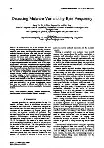
D. The Value of Threshold In order to attain the effective and applicable thresholds of the similarity and the distance, we do a training experiment. In this experiment, all test samples are divided into two groups. In the first group, there are 66 samples, all of which are identified by popular anti-virus tools to be malware Trojan-GameThief.Win32.OnLineGames.ttgu. The second group consists of 538 malware samples, which are not considered as the variants of the first group, and 266 non-malware samples. To get a threshold keeping the misjudgment rate as low as possible, we do not add any variant of Trojan-


IV. PRIMARY EXPERIMENTAL RESULTS In following experiments, if not mentioned specially, all the malware is detected and named by Kaspersky Internet Security 2009 (KIS2009) which is updated on March 2, 2009 [13]. All the experiment samples, including the malwares and non-malwares, are not packed. So before the experiment, some of them have been unpacked using SUCOP’s VM Unpacker. This is because, as we mentioned previously, the identification of packed malware is beyond the BFBDM's ability. We pack one random chosen executable file with UPX 3.03 with default setting, and compare the packed file with the original file. The distance is 623.928681822 and the similarity is 0.725564758941, which indicates that the byte frequency varies greatly between them. A. Some Definitions In this section, we give some useful and essential definitions in the following experiments. Base sample: when comparing many samples with one sample, we call the one compared sample base sample. Comparing two samples, the result should be one of the following three: (1) Detected (D): the BFBDM detects the two samples as the same software. (2) Suspicious (S): the two samples are suspicious to be the same. (3) Not (N): according the BFBDM, the two samples are not the same. © 2011 ACADEMY PUBLISHER

same malware different software

20000 19000 18000 17000 16000 15000 14000 13000 12000

Distance

GameThief.Win32.OnLineGames.ttgu into this training set. The result is shown in the Fig. 1. In the Fig. 1, the red points denote the samples in the first group, and the black ones denote the samples in the second group. All the red points have high similarity and low distance, while contrastively the black ones have low similarity and high distance. The points with distance higher than 20,000, which are not displayed in the Fig.1, are all the black. Distinctively, all the red points concentrate in a small range, which is close to the point (1, 0) and surrounded by the magenta dashed line. Additively, we randomly choose 10 pairs of samples, and calculate the distance and similarity between them. The two samples in each pair have the same file size, but hold no affinity. The result is shown in the following table 3. Thus, from the result, there is little probability that two executable files without any relationship will have short distance and high similarity. Based upon the experiment result, we find that if Dis ( N , M ) ≤ 1000 and Sim( N , M ) ≥ 0.999 , the two files almost denote the same software. If Dis ( N , M ) ≤ 5000 and Sim( N , M ) ≥ 0.99 , the two files are suspicious to be the same. However, If Dis ( N , M ) > 5000 or Sim( N , M ) < 0.99 , there is a weak correlation between these two samples. In the following experiments, we will adopt these standards to determine if the testing samples are malware variants.

641

11000 10000 9000 8000 7000 6000 5000 4000 3000 2000 1000 0 0.0

0.1

0.2

0.3

0.4

0.5

0.6

0.7

0.8

0.9

1.0

Similarity

Figure 1. Result of the Training (Note: the points with distance higher than 20,000 are not displayed) TABLE III. RESULTS OF RANDOM CHOICE Result Distance Similarity

Minimum

Median

Maximum

Average

180.616

1452.998

2850.212

1644.292

0.484

0.798

0.920

0.760

False negative rate: the possibility to misjudge the malware as non-malware. Assuming there are m malwares tested, and n out of them are detected as nonmalware, the false negative rate is n/m. False positive rate: the possibility to misjudge the nonmalware as malware. Assuming there are m nonmalwares tested, d out of them are detected as malware, and s out of them are detected as suspicious, the false positive rate is (d+s)/m. Detection rate: the possibility to identify an unknown variant type of a known malware. Assuming there are v types of malware variants, which are variants from the same one known malware, and d types out of v are detected as malware, the detection rate is d/v. B. Experiments to Test the False Negative Rate and False Positive Rate The basic purpose of a malware detection model is that, giving one malware sample, the model can detect out the other malware samples which have the completely same instructions with the given sample. An important and primary requirement of the malware detection model is that it must keep the false positive rate as low as possible. In other words, the detection model should never detect the non-malware as malware. In this section, we do five experiments to testify the BFBDM’s false negative rate and false positive rate. Firstly, in the experiment 1-1, we choose 92 samples of malware named Trojan-GameThief.Win32.Magania.amjb. All of them are different in MD5 checksum, which indicates that they all are different. If not mentioned specially, so are all the following other testing samples. We randomly choose one of them as the base sample, and

642


Exp. 1-1 Exp. 1-2 Exp. 1-3 Exp. 1-4

20000 19000 18000 17000 16000 15000 14000 13000 12000

Distance

compare the others with this specific base sample. The result is shown in the table 4 and Fig. 2. In the Fig. 2, every point indicates one sample’s distance and similarity calculated with the base one. The X-axis means the similarity, while the Y-axis means the corresponding distance between the two samples. According to the BFBDM, it seems that all the tested samples are detected as the same as the base sample malware. Therefore, the false negative rate of our novel model in this experiment is 0%. Secondly, in experiment 1-2, we choose 199 samples of the malware Trojan-Dropper.Win32.Agent.yux. We randomly choose one of them as the base sample, compare the others with the base sample, and get the result shown in the table 4 and Fig. 2. According to the model, we can conclude that all these 199 samples belong to the same malware. The result from our model is the same as that from KIS2009. In this experiment, the false negative rate is also 0%. Thirdly, in experiment 1-3, in order to test the BFBDM’s false positive rate, we choose 456 nonmalware samples, which are randomly collected from the windows directory. The base sample is the same as that used in the experiment 1-2. Then, we compare them with the base malware sample. The experiment result is shown in the table 4 and Fig. 2. Clearly in this experiment, all the tested samples are detected as not the same as the base one. That is, all tested samples are non-malware. Therefore, the false positive rate of BFBDM in this experiment is 0%. Fourthly, in the experiment 1-4, we calculate the distance and the similarity among one non-malware and other 2926 malware samples. In our experiment, we choose the windows edit tool, notepad.exe, as the base sample. Then we get the result shown in the table 4 and Fig. 2. Clearly, none of the malware is considered as the notepad.exe or the notepad.exe’s variant. The false positive rate of BFBDM in this experiment is also 0%. The experiment results in 1-1 and 1-2 show that among the samples of the same malware there are short distance and high similarity. Contrastively, in the experiments 1-3 and 1-4, the distance is long and the similarity is low. In the Fig. 2, the overlapping points of experiments 1-1 and 1-2 are concentrated in a small range, which is very close to the point (1, 0) and surrounded by the magenta dashed line, while these of experiments 1-3 and 1-4 are far from the point (1, 0). In table 5, we summarize the four previous experiments. In all experiments in this section previously, our model has a false negative rate of 0% and a false positive rate of 0%. In this respect, the BFBDM is as effective as the traditional signatures. Furthermore, in the experiment 1-5, we randomly choose 2,796 malware samples and 10,764 non-malware and non-exe samples. Then we calculate the distance and similarity between each non-malware and malware. The result shows that, in these 30,096,144 compares, only 136 pairs of samples are detected as holding affinity. Thus in this experiment, the false positive rate is 0.0004519%.


11000 10000 9000 8000 7000 6000 5000 4000 3000 2000 1000 0 0.0

0.1

0.2

0.3

0.4

0.5

0.6

0.7

0.8

0.9

1.0

Similarity

Figure 2. Distribution of the Distance and Similarity of experiments 11, 1-2, 1-3 and 1-4 (Note: the points with distance higher than 20,000 are not displayed)

TABLE IV. EXPERIMENT RESULTS OF 1-1, 1-2, 1-3 AND 1-4 Exp. 1-1

Exp. 1-2

Exp. 1-3

Exp. 1-4

Dis≤500

91

198

0

0

500＜Dis≤1000

0

0

0

0

1000＜Dis≤2500

0

0

0

1

2500＜Dis≤5000

0

0

0

1187

5000＜Dis≤10000

0

0

323

1445

10000＜Dis

0

0

133

291

91

198

456

2924

Range

Total

a. The distribution of the Distance Exp. 1-1

Exp. 1-2

Exp. 1-3

Exp. 1-4

0≤Sim＜0.9

0

0

455

2915

0.9≤Sim＜0.99

0

0

1

9

0.99≤Sim＜0.999

0

0

0

0

0.999≤Sim＜0.9999

86

193

0

0

0.9999≤Sim＜0.99999

0

0

0

0

0.99999≤Sim≤1

5

5

0

0

Total

91

198

456

2924

Range

b. The distribution of the Similarity

At last, in the experiment 1-6, on the base of the experiment 1-1, we calculate the distance and similarity between every two samples used in the experiment 1-1. The result is shown in the table 6. In the result, all the distance is shorter than 1,000, and all the similarity is higher than 0.999. Therefore, with any sample as the base sample, using the BFBDM, the other same samples can be identified with the false negative rate of 0%. In other words, in our BFBDM model, the


643

choice of the base sample does not influence its validity. So in real life application, any sample, of one type of malware, can be considered to be the base sample of that type. This important feature greatly improves the applicability of our new approach.

400 380 360 340

Distance

320

TABLE V. SUMMARY OF SECTION 4.2

300 280 260 240

Exp. 1-1

Exp. 1-2

Exp. 1-3

Exp. 1-4

False Negative Rate

0%

0%

N/A

N/A

False Positive Rate

N/A

N/A

0%

0%

Exp

220 200 0.9988 0.9989 0.9990 0.9991 0.9992 0.9993 0.9994 0.9995 0.9996 0.9997 0.9998 0.9999 1.0000

Similarity

Figure 3. Distribution of the distance and similarity in experiments 2-1 TABLE VI. EXPERIMENTAL RESULTS OF 1-6 Minimum

Median

Maximum

Average

Distance

2.8284

210.4804

293.1109

203.2321

Similarity

0.9991

0.9995

1

0.9995

Result

C. Experiments to Verify the Ability to Detect the Malware Variants Besides the low false negative rate and the low false positive rate, to the malware detection model, it also requires that, giving a malware, the model can detect as many variants of the given one as possible. In this section, three experiments are used to verify the BFBDM’s ability to detect the malware variants. In experiment 2-1, on the base of the malware TrojanDropper.Win32.Agent.yux, the other 24 types of malware variants we collected can be detected. We estimate the distance and similarity between these variants and the base sample, and use the BFBDM to get the result shown in the table 7 and Fig. 3. In the table 7, the prefix of some malwares’ name, “Trojan-”, is ignored. In this experiment, approximately, 98.56% of the tested samples are identified as the same as the base sample. The other 12 exceptions are detected as suspicious. That is, when we have a sample of the TrojanDropper.Win32.Agent.yux, all the other 24 kinds of variants can be detected out. But this does not mean that the BFBDM can detect all the variants of the base malware, TrojanDropper.Win32.Agent.yux. We check the proximity between the base sample and other 40 kinds of variants of Trojan-Dropper.Win32.Agent.yux. The result shows that none of these 40 kinds can be detected base upon the Trojan-Dropper.Win32.Agent.yux. Thus, in this case, on the scope of our data sets, the detection rate is 37.5%. In sum, base upon the known malware samples, the BFBDM can detect some variants but not all. Even so, the BFBDM is, to some extent, better than the signature based detection model. In above experiments, all the variants are identified by popular anti-virus software. In the following two experiments, we want to test whether our model can detect some variants which are not identified by popular anti-virus software.


TABLE VII. EXPERIMENTAL RESULTS OF 2-2 Malware

Gross

D*

S*

N*

Dropper.Win32.Agent.aahc

47

47

0

0

Dropper.Win32.Agent.aain

29

19

10

0

Dropper.Win32.Agent.aaot

23

23

0

0

Dropper.Win32.Agent.aarc

28

27

1

0

Dropper.Win32.Agent.zen

98

98

0

0

Dropper.Win32.Agent.zep

17

17

0

0

Dropper.Win32.Agent.zlk

106

106

0

0

Trojan.Win32.Agent.amtx

8

8

0

0

GameThief.Win32.Magania.akee

21

21

0

0

GameThief.Win32.Magania.akvj

4

4

0

0

GameThief.Win32.Magania.akxf

5

5

0

0

GameThief.Win32.Magania.akxm

14

14

0

0

GameThief.Win32.Magania.alod

88

88

0

0

GameThief.Win32.Magania.alrj

3

3

0

0

GameThief.Win32.Magania.alzm

6

6

0

0

GameThief.Win32.Magania.amhc

8

7

1

0

GameThief.Win32.Magania.amjb

92

92

0

0

GameThief.Win32.Magania.amlc

25

25

0

0

GameThief.Win32.Magania.appe

83

83

0

0

GameThief.Win32.OnLineGames.toyj

1

1

0

0

GameThief.Win32.OnLineGames.tquw

16

16

0

0

GameThief.Win32.OnLineGames.tqvn

54

54

0

0

GameThief.Win32.OnLineGames.tqza

55

55

0

0

GameThief.Win32.OnLineGames.tvck

4

4

0

0

835

823

12

0

Total

In experiment 2-2, there are two samples. One of them is detected as non-malware by Eset NOD32 2.70.27 updated on March 13, 2009 [14], while Backdoor.Win32.Hupigon.ermp by KIS2009. And the other one is detected as

644

Win32/TrojanDownloader.Delf.OKS by NOD32, while Backdoor.Win32.Hupigon.eykf by KIS2009. When we check the correlation between these two samples, we find there are short distance of 1624.61903227 and high similarity of 0.999816644416 between them. Then we check them on the website VirusTotal with 39 antivirus engines [15], for more information on March 17, 2009. Among the 39 antivirus engines, there are 32 engines considering the former sample as malware, while 33 the latter. Ignoring the result without a certain name, such as suspicious, heuristic, generic, unknown, and so on, there are 15 engines treating them as the same malware or variants of one malware. And 7 other engines consider them as different. According to the data from VirusTotal, it seems that these two samples should be variants of the same malware. It’s also observed that the former sample is detected as non-malware by Eset NOD32 2.70.27, and probably a variant of Win32/Hupigon by Eset NOD32 4.0.314.0 with the same virus database of version 3941. In experiment 2-3, we consider two special samples. One of them is considered as non-malware by the KIS2009, while the other TrojanDropper.Win32.Agent.zgu. Firstly, we compute the distance and the similarity between these two softwares. Surprisingly we find out the two softwares have a strong correlation. The distance between them is 77.6337555449, and the similarity is 0.999999223745. Then, we check them on the website VirusTotal on March 17, 2009. Three engines, AntiVir 7.9.0.116, Avast 4.8.1335.0 and McAfee-GW-Edition 6.7.6, detect them as the same malware. The AntiVir names them as TR/StartPage.fxc, Avast Win32:Agent-AEFX, and McAfee-GW-Edition Trojan.StartPage.fxc. In addition, The AVG 8.0.0.237 treats them as the same Win32/PolyCrypt, and the BitDefender 7.2 and the GData 19 name them as the same Trojan.Heur.AutoIT.1. None of the engines indicates that they are different. Finally, we use the software C32ASM to disassembly these two executable files and inspect them carefully. The result shows that their assembly codes are completely the same. After computing their MD5 digest, it shows that their MD5 values are different. Therefore, it’s clear that the differences only exist in their data section. Clearly we can confirm that these two softwares have the same structure and function. That is, these two executable files are totally the same. In the experiments 2-1, on the base of a sample of Trojan-Dropper.Win32.Agent.yux, the BFBDM is successful to detect 24 other types of malware variants. In the experiments 2-2 and 2-3, the BFBDM also successfully detects out the malware variants, while the Eset NOD32 2.70.27 and the KIS2009 fail to identify the corresponding samples. In other words, our novel approach has more merits than current popular industrial anti-malware tools when identifying malware variants.



V. ALGORITHM COMPLEXITY For comparing one sample with the base one, the algorithm description is shown as the following. Input: the comparing sample’s full name Output: the distance and similarity between the base sample and the comparing sample /*Function: calculate the distance and similarity between the base sample and a given one*/ 01 Open comparing sample file in binary mode 02 Read 512 more bytes in the opened file 03 While not the end of the file{ 04 For each byte read{ 05 dic[(int)byte] += 1 06 } 07 Read 512 more bytes in the opened file 08 } 09 For each i between 1 and 256 && i != 90{ 10 dot_metrix += basedic[i]* dic [i] 11 dis1 += basedic[i]**2 12 dis2 += dic [i]**2 13 dis += (dic [i]- basedic[i])**2 14 } 15 similarity =dot_metrix/(sqrt(dis1*dis2) ) 16 distance = sqrt(dis)

The dictionary basedic, which stores the byte frequency information of the base sample, is prepared in advance. The dictionary dic is used to get and store the information of the comparing sample. The items of dic are set to 0 initially. For a file with size of n bytes, the step 02 and 07 will be executed by n/512 times. The process to get and store the byte frequency information in the step 05 will be executed by n times. Constantly, for calculating the distance and similarity, each step in the loop, from the step 10 to the step 13, will be executed by 254 times. So processing a file of n bytes, the asymptotic time complexity of the BFBDM is T(n)=O(n). Dealing with a file of n bytes, this process needs a buffer of 512 bytes to get the file’s content, two dictionaries of 256 items to store the byte frequency information, and some bytes of constant amount to store the temporary variable and the result. So the asymptotic space complexity of this process is S(n)=O(1). In an implementation with python 3.01 of single thread, we do some experiments to test the BFBDM’s efficiency in the actual use, and get the result in the table 8. Every round of this experiment runs three times, and the arithmetic average value of three times’ results is used as the final result. The “Read File” is the step 02 and 07 in the algorithm description, the “Get Byte Frequency” from the step 04 to the step 06, and the “Calculate” from the step 09 to the step 16. The byte frequency information of the compared files is got in advance and stored in memory, while that of the comparing files is read and counted on need. From the result, the phase “Read File” and the phase “Get Byte Frequency”, whose efficiency is strongly determined by the I/O performance of the hard disk and memory, are the bottlenecks of the whole process. The phase “Get Byte Frequency” is also influenced by the implementation itself. And calculating the distance and similarity between two files takes only about 1.26ms averagely.


645

In general, the BFBDM’s algorithm complexity is low. TABLE VIII. PERFORMANCE OF BFBDM

[6] Round

Items

1

2

3

[7]

1 file

1 file

150 files

Total Size(bytes)

66,560

66,560

59,489,928

Average Size(bytes)

66,560

66,560

396,600

1

2000

2000

Total(ms)

1.866

1.845

1497.719

Mean(ms/file)

1.866

1.845

9.985

[9]

Total(ms)

41.948

42.929

43842.543

[10]

Mean(ms/file)

41.948

42.929

292.284

Total(ms)

1.31

2511.683

378116.144

Mean(ms/calculate)

1.31

1.256

1.26

Count

Comparing File

[5]

[8] Compared File Count Read File

Get Byte Frequency

Calculate

[11]

VI. CONCLUSION The experiments show our novel BFBDM can be used to detect the malware with a low false negative rate and a low false positive rate. And the BFBDM has the ability to detect the malware variants, to the extent where is much beyond that the traditional malware variants detection model can reach. Furthermore, the BFBDM can be used to identify the proximity of two executable files. During the experiments, it’s found that, the stronger the correlation exists between two executable files, the shorter the distance is, and the higher the similarity is. REFERENCES [1] [2]

[3]

[4]

Wikipedia, Malware, http://en.wikipedia.org/wiki/Malware, 2009 Alexander Gostev, Kaspersky Security Bulletin: Statistics 2008, http://www.viruslist.com/en/analysis?pubid=204792052, Mar 02 2009. Sergey Golovanov, Alexander Gostev, Vitaly Kamluk, and Oleg Zaitsev, Kaspersky Security Bulletin: Malware evolution 2008, http://www.viruslist.com/en/analysis?pubid=204792051, Mar 02 2009. ESET, Virus Threats and Analysis, http://www.virusradar.com/index_enu.html, 2009.


[12]

[13] [14] [15]

Ismael Briones, Aitor Gomez, “Graph, Entropy and Grid Computing: Automatic Comparison of Malware”, Virus Bulletin 2008, Ottawa. 2008. M Dalla Preda, M Christodorescu, S Jha, and S Debray, “A Semantics-Based Approach to Malware Detection”, ACM Transactions on Programming Languages and Systems, ACM, New York, Aug. 2008, Article No. 25. Christodorescu, M., Jha, S., Seshia, S.A., Song, D., and Bryant, R.E. “Semantics-aware malware detection”, IEEE Security and Privacy 2005, http://www.thehackademy.net/madchat/vxdevl/papers/ave rs/oakland05.pdf , May 2005. E Kirda, C Kruegel, G Banks, G Vigna, and RA Kemmerer, Behavior-based spyware detection, 15th USENIX Security Symposium, USENIX, Berkeley CA, Jun. 2006, pp. 273–288. Peter Szor, The art of computer virus research and defense, Addison-Wesley Professional, 2005. R Lyda, abd J Hamrock, “Using entropy analysis to find encrypted and packed malware”, IEEE Security and Privacy 2007, http://wwwcsif.cs.ucdavis.edu/~madl/packed.pdf, Apr. 2007. Christopher Kruegel, Engin Kirda, Darren Mutz, William Robertson, and Giovanni Vigna, Polymorphic worm detection using structural information of executables. Recent Advances in Intrusion Detection, Springer, Heidelberg, 2006, pp. 207-226. Mihai Christodorescu, and Somesh Jha, “Static Analysis of Executables to Detect Malicious Patterns”, USENIX Security Symposium, USENIX Association, Berkeley CA, 2003, pp. 169-186. Kaspersky Lab, http://www.kaspersky.com/, 2009. ESET, http://www.eset.com/, 2009. VirusTotal, http://www.virustotal.com/, 2009.

Sheng Yu was born in Sichuan, China on June 24, 1985. In 2007 and 2010 respectively, he got the Bachelor of Engineering (B.E.) degree and Master of Engineering (M.E.) degree both in School of Computer Science and Engineering at University of Electronic Science and Technology of China (UESTC). He was major in information security in undergraduate period, and information and communication engineering in master stage. Currently, he is studying in UESTC seeking for a Ph.D degree. Since 2007, he works in the Network and Data Security Key Laboratory of Sichuan Province, Chengdu, China. His previous research interest is information security. Currently, his research interests are bioinformatics and social networking.