Detecting Overlapping Communities in Networks Using Spectral ...

Detecting Overlapping Communities in Networks Using Spectral Methods

arXiv:1412.3432v4 [stat.ML] 12 Mar 2015

Yuan Zhang, Elizaveta Levina and Ji Zhu

Abstract Community detection is a fundamental problem in network analysis. In practice, communities often overlap, which makes the problem more challenging. Here we propose a general, flexible, and interpretable generative model for overlapping communities, which can be viewed as generalizing several previous models in different ways. We develop an efficient spectral algorithm for estimating the community memberships, which deals with the overlaps by employing the K-medians algorithm rather than the usual K-means for clustering in the spectral domain. We show that the algorithm is asymptotically consistent when networks are not too sparse and the overlaps between communities not too large. Numerical experiments on both simulated networks and many real social networks demonstrate that our method performs well compared to a number of benchmark methods for overlapping community detection.

1

Introduction

The problem of community detection in networks has been actively studied in several distinct fields, including physics, computer science, statistics, and the social sciences. Its applications include understanding social interactions of people (Zachary, 1977; Resnick et al., 1997) and animals (Lusseau et al., 2003), discovering functional regulatory networks of genes (Bolouri and Davidson, 2010; Zhang, 2009) and even designing parallel computing algorithms (Chamberlain et al., 1998; Hendrickson and Kolda, 2000). Community detection is in general a challenging task. The challenges include defining what a community is (commonly taken to be a group of nodes that have more connections to each other than to the rest of the network, although other types of communities are not unusual), formulating realistic and tractable statistical models of networks with communities, and designing fast scalable algorithms for fitting such models. In this paper, we focus on network models with overlapping communities, with nodes potentially belonging to more than one community at a time. This is common in real-world networks (Palla et al., 2005; Pizzuti, 2009), and yet most literature to date has focused on partitioning the network into non-overlapping communities, with some notable exceptions discussed below. Our goal is to design an overlapping community model that is flexible, interpretable, and computationally feasible. We will thus focus on models which can be fitted by spectral methods, one of the most scalable tools for fitting non-overlapping community models available to date. We start with a brief review of relevant work in community detection for non-overlapping communities, which mainly falls into one of two broad categories: algorithmic methods, based on optimizing some criterion reflecting desirable properties of a partition over all possible partitions (see Fortunato (2010) for a review), and model fitting, where a generative model with communities is postulated for the network and its parameters are estimated from the observed adjacency matrix 1

(see Goldenberg et al. (2010) for a review). Perhaps the most popular and best studied generative model for community detection is the stochastic block model (SBM) (Holland and Leinhardt, 1981; Holland et al., 1983). The SBM views the n × n network adjacency matrix A, defined by Aij = 1 if there is an edge between i and j and 0 otherwise, as a random graph with independent Bernoullidistributed edges. The Bernoulli probabilities for the edges depend on the node labels ci which take values in {1, . . . , K}, and the K × K matrix B containing the probabilities of edges forming between different communities. The node labels can be represented by an n × K binary community membership matrix Z with exactly one “1” in each row, Zik = 1[ci = k] for all i, k. Then the probabilities of edges are given by W ≡ E(A) = ZBZ T . Thus in this model, a node’s label determines its behavior entirely, and thus all nodes in the same community are “stochastically equivalent”, and in particular have the same expected degree. This is known to be often violated in practice, due to commonly present “hub” nodes with many more connections than other nodes in their community. The degree-corrected stochastic block model (DCSBM) (Karrer and Newman, 2011) was proposed to address this limitation, which multiplies the probability of an edge between nodes i and j by the product of node-specific positive “degree parameters” θi θj . Both SBM and DCSBM can be consistently estimated by maximizing the likelihood (Bickel and Chen, 2009; Zhao et al., 2012), but directly optimizing the likelihood over all label assignments is not computationally feasible. A number of faster algorithms for fitting these models have been proposed in recent years, including pseudo-likelihood (Amini et al., 2013), belief propagation (Decelle et al., 2012), spectral approximations to the likelihood (Newman, 2013; Le et al., 2014), and generic spectral clustering (Von Luxburg, 2007), used by many and analyzed, for example, in Rohe et al. (2011); Sarkar and Bickel (2013), and Lei and Rinaldo (2013). It was further shown that regularization improves on spectral clustering substantially (Amini et al., 2013; Chaudhuri et al., 2012), and its theoretical properties have been further analyzed by Qin and Rohe (2013) and Joseph and Yu (2013). While for specific likelihoods one can develop methods that are both fast and more accurate than spectral clustering, such as the pseudo-likelihood (Amini et al., 2013), in general spectral methods remain the most scalable option available. While the majority of the existing models and algorithms for community detection focus on discovering non-overlapping communities, there has been a growing interest in exploring the overlapping scenario, although both extending the existing models to the overlapping case and developing brand new models remain challenging. Like methods for non-overlapping community detection, most existing approaches for detecting overlapping communities can be categorized as either algorithmic or model-based methods. Model-based methods focus on specifying how node community memberships determine edge probabilities. For example, the overlapping stochastic block model (OSBM) (Latouche et al., 2009) extends the SBM by allowing the entries of the membership matrix Z to be independent Bernoulli variables, thus allowing multiple “1”s in one row, or all “0”s. The mixed membership stochastic block model (Airoldi et al., 2008) draws membership vectors Zi· from a Dirichlet prior. The membership vector is drawn again to generate every edge, instead of being fixed for the node, so the community membership for node i varies depending on which node j it is interacting with. The “colored edges” model (Ball et al., 2011), sometimes referred to as the Ball-Karrer-Newman model or BKN, allows continuous community membership by relaxing the binary Z to a matrix with non-negative entries (with some normalization constraints for identifiability), and discarding the matrix B. The Bayesian nonnegative matrix factorization model (Psorakis et al., 2011) is related to the model but with notable differences. Algorithmic methods for overlapping community detection mostly rely on local greedy searches

2

and intuitive criteria. Current approaches include detecting each community separately by maximizing a local measure of goodness of the estimated community (Lancichinetti et al., 2011) and updating an initial estimate of the community membership by neighborhood vote (Gregory, 2010). Local methods typically rely heavily on a good starting value. Global algorithmic approaches include computing a non-negative matrix factorization approximation to the adjacency matrix and extracting a binary membership matrix from one of the factors (Wang et al., 2011; Gillis and Vavasis, 2012). Many heuristic methods do not take heterogeneous node degrees into account, and we found empirically they can perform poorly in the presence of hubs (see Section 5). In this paper, we propose a new generative model for overlapping communities, the overlapping continuous community assignment model (OCCAM). It allows a node to belong to different communities to a different extent, via the membership vector Zi· with non-negative entries which represent how strongly a node is associated with various communities. We also allow arbitrary degree distributions in a manner similar to the DCSBM, and retain the K × K matrix B which allows to interpret connections between communities and compare them. All the model parameters (membership vectors, degree corrections, and community-level connectivity) are identifiable under certain constraints which we will state explicitly. We also develop a fast spectral algorithm to fit OCCAM. Typically, spectral clustering projects the adjacency matrix or its Laplacian onto the K leading eigenvectors representing the nodes’ latent positions, and performs K-means in that lower-dimensional space to estimate community memberships. Our key insight here is that when the nodes come from a mixture of clusters (as they would with multiple community memberships), K-means has no chance of recovering the cluster centers correctly; but as long as there are enough pure nodes in each community, K-medians will still be able to identify the cluster centers correctly by ignoring the “mixed” nodes on the boundaries. We show that our method produces asymptotically consistent parameter estimates as the number of nodes grows as long as there are enough pure nodes and the network is not too sparse. We also employ a simple regularization scheme, since it is by now well known that regularizing spectral clustering substantially improves its performance, especially in sparse networks (Chaudhuri et al., 2012; Amini et al., 2013; Qin and Rohe, 2013). We provide an explicit rate for the regularization parameter, implied by our consistency analysis, and show that the overall performance is robust to the choice of the constant multiplier in the regularization parameter as long as the rate is specified correctly. The rest of the paper is organized as follows. We introduce the model and discuss parameter identifiability in Section 2, present the two-stage spectral clustering algorithm in Section 3, and state consistency results and describe the choice of the regularization parameter in Section 4. Some simulation results are presented in Section 5, where we investigate robustness of our method to the choice of regularization parameter and compare it to a number of benchmark methods for overlapping community detection. We apply the proposed method to a large number of real social ego-networks (networks consisting of all friends of one or several users) from Facebook, Twitter, and GooglePlus in Section 6. Section 7 concludes the paper with a brief discussion of contributions, limitations, and future work. All proofs are given in the supplemental materials.

3

2

The overlapping continuous community assignment model

2.1

The model

Recall that we represent the network by its n × n adjacency matrix A, a binary symmetric matrix with {Aij , i < j} independent Bernoulli variables and W ≡ E(A). We will assume that W has the form W = αn ΘZBZ T Θ . (2.1) We call this formulation the Overlapping Continuous Community Assignment Model (OCCAM). The factor αn is a global scaling factor that controls the overall edge probability, and the only component that depends on n. As is commonly done in the literature, for theoretical analysis we will let αn → 0 at a certain rate, otherwise the network becomes completely dense as n → ∞. The n × n diagonal matrix Θ = diag(θ1 , . . . , θn ) contains non-negative degree correction terms that allow for heterogeneity in the node degrees, in the same fashion as under the DCSBM. We will later assume that θi ’s are generated from a fixed distribution FΘ which does not depend on n. The n × K community membership matrix Z is the primary parameter of interest; the i-th row Zi· represents node i’s propensities towards each of the K communities. We assume Zik ≥ 0 for all i, k, and kZi· k2 = 1 for identifiability. Formally, a node is “pure” if Zik = 1 for some k. Later, we will also assume that the rows Zi· ’s are generated independently from a fixed distribution FZ that does not depend on n. Finally, the K × K matrix B represents (scaled) probabilities of connections between pure nodes of all communities. Since we are already using αn and Θ, we constrain all diagonal elements of B to be 1 for identifiability. Other constraints are also needed to make the model fully identifiable; we will discuss them in Section 2.2. Note that the general form (2.1) can, with additional constraints, incorporate many of the other previously proposed models as special cases. If all nodes are pure and Z has exactly one “1” in each row, we get DCSBM; if we further assume all θi ’s are equal, we have the regular SBM. If the constraint kZi· k2 = 1 is removed and the entries of Z are required to be 0 or 1, and all θi ’s are equal, we have the OSBM of Latouche et al. (2009). Alternatively, if we set B = I, we have the “colored edges” model of Ball et al. (2011). Our model is also related to the random dot product model (RDPM) (Nickel, 2007; Young and Scheinerman, 2007), which stipulates W = X0 X0T for some (usually low-rank) X0 . This is true for our model if B is semi-positive definite, since then we √ can uniquely define X0 = αn ΘZB 1/2 . OCCAM is thus more general than all of these models, and yet is fully identifiable and interpretable.

2.2

Identifiability

The parameters in (2.1) obviously need to be constrained to guarantee identifiability of the model. All models with communities, including the SBM, are considered identifiable if they are identifiable up to a permutation of community labels. To show the interplay between the model parameters, we first state identifiability conditions treating all of αn , Θ, Z, and B as constant parameters, and then discuss what happens if Θ and Z are treated as random variables as we do in the asymptotic analysis. The following conditions are sufficient for identifiability: I1 B is full rank and strictly positive definite, with Bkk = 1 for all k. I2 All Zik ≥ 0, kZi· k2 = 1 for all i = 1, . . . , n, and there is at least one “pure” node in every community, i.e., for each k = 1, . . . , K, there exists at least one i such that Zik = 1. 4

I3 The degree parameters θ1 , . . . , θn are all positive and n−1

Pn

i=1 θi

= 1.

Theorem 2.1. If conditions (I1), (I2) and (I3) hold, the model is identifiable, i.e., if a given probability matrix W corresponds to a set of parameters (αn , Θ, Z, B) through (2.1), these parameters are unique up to a permutation of community labels. The proof of Theorem 2.1 is given in the supplemental materials. In general, identifiability is non-trivial to establish for most overlapping community models, since, roughly speaking, an edge between two nodes can be explained by either their common memberships in many of the same communities, or the high probability of edges between their two different communities, a problem that does not occur in the non-overlapping case. Among previously proposed models, the OSBM was shown to be identifiable (Latouche et al., 2009), but their argument does not extend to our model since they only considered Z with binary entries. The identifiability of the BKN model was not discussed by Ball et al. (2011), but it is relatively straightforward (though still non-trivial) to show that it is identifiable as long as there are pure nodes in each community. While Theorem 2.1 makes the model in (2.1) well defined, it is also common practice in the community detection literature to treat some of the model components as random quantities. For example, Holland et al. (1983) treat community labels under the SBM as sampled from a multinomial distribution, and Zhao et al. (2012) treat the degree parameters θi ’s in DCSBM as sampled from a general discrete distribution. For our consistency analysis, treating θi ’s and Zi· ’s as random significantly simplifies conditions and allows for an explicit choice of rate for the tuning parameter τn , which will be defined in Section 3. We will thus treat Θ and Z as random and independent of each other for the purpose of theory, assuming that the rows of Z are independently generated from a distribution FZ on the unit sphere, and θi ’s are i.i.d. from a distribution FΘ on positive real numbers. The conditions I2 and I3 are then replaced with the following two conditions, respectively: RI2 FZ = πp Fp + πo Fo is a mixture of a multinomial distribution Fp on K categories for pure nodes and an arbitrary distribution Fo on {z ∈ RK : zk ≥ 0, kzk2 = 1} for nodes in the overlaps, and πp >  > 0. R∞ RI3 FΘ is a probability distribution on (0, ∞) satisfying 0 t dFΘ (t) = 1. The distribution Fo can in principle be any distribution on the positive quadrant of the unit sphere. For example, one could first specify that with probability πk1 ,...,km , node i belongs to communities {k1 , . . . , km }, and then set Zik = √1m 1(k ∈ {k1 , . . . , km }). Alternatively, one could generate values for the m non-zero entries of Zi· from an m-dimensional Dirichlet distribution, and set the rest to 0.

3

A spectral algorithm for fitting the model

The primary goal of fitting this model is to estimate the membership matrix Z from the observed adjacency matrix A, although other parameters may also be of interest. Since computational scalability is one of our goals, we focus on algorithms based on spectral decompositions, one of the most scalable approaches available. Recall that spectral clustering typically works by first representing all data points (the n nodes) by an n × K matrix X consisting of leading eigenvectors of a matrix derived from the data, which we call G for now, and then applying K-means clustering 5

to the rows of X. For example, under the SBM, the matrix G should be chosen to have eigenvectors X that approximate the eigenvectors X0 of W = E(A) as closely as possible, since the eigenvectors of W are piecewise constant and contain all the community information. A naive choice G = A is intuitively appealing, though it has been shown in practice and in theory (Sarkar and Bickel, 2013) that the graph Laplacian of A, i.e., L = D −1/2 AD −1/2 , where D = diag(A1), is a better choice, or, for sparse graphs, different regularized versions of L (Amini et al., 2013; Chaudhuri et al., 2012; Qin and Rohe, 2013; Joseph and Yu, 2013). An additional step of normalizing the rows of X before performing K-means is often appropriate if the underlying model is assumed to be the degree-corrected stochastic blockmodel (Qin and Rohe, 2013). Regardless of the matrix chosen to estimate the eigenvectors of W , the key difference between the regular SBM under which spectral clustering is usually studied and our model is that under the SBM there are only K unique rows in X0 , and thus K-means can be expected to accurately cluster the rows of X, which is a noisy version of X0 . Under our model, the rows of X0 are linear combinations of the “pure” rows corresponding to “centers” of the K communities. Thus even if we could recover X0 exactly, K-means is not expected to work, and it is in fact straightforward to show that the K-means algorithm does not recover the positions of pure nodes correctly unless non-pure nodes either vanish in proportion or converge to pure nodes’ latent positions as n grows (proof omitted here as it is not needed for our main argument). The key idea of our algorithm is to replace K-means with K-medians clustering: if the proportion of pure nodes is not too low, then the latent positions of the cluster centers can still be recovered correctly, and therefore the coefficients of mixed nodes can be estimated accurately by projecting onto the pure nodes. Other details of the algorithm involve regularization and normalization that are necessary for dealing with sparse networks and heterogeneous degrees. Our algorithm for fitting the OCCAM takes as input the adjacency matrix A and a regularization parameter τn > 0 which we use to regularize the estimated latent node positions directly. This is easier to handle technically than regularizing the Laplacian, and we will give an explicit rate for τn that guarantees asymptotic consistency in Section 4. The algorithm proceeds as follows: ˆ AL ˆ AU ˆ T , where L ˆ A is the K × K diagonal matrix containing the K leading 1. Compute U A ˆ A is the n × K matrix containing the corresponding eigenvectors. eigenvalues of A, and U While the true W = E(A) is positive definite, in practice some of the eigenvalues of A may ˆ ≡ U ˆ AL ˆ 1/2 be the estimated be negative; if that happens, we truncate them to 0. Let X A latent node positions. ˆ ∗ , a normalized and regularized version of X, ˆ the rows of which are given by 2. Compute X 1 ∗ ˆ ˆ Xi· = ˆ Xi· . kXi· k2 +τn

ˆ ∗ and obtain K estimated cluster centers 3. Perform K-medians clustering on the rows of X K s1 , . . . , sK ∈ R , i.e., n

1X

ˆ∗

{s1 , . . . , sK } = arg min min

Xi· − s s1 ,...,sK n 2 s∈{s1 ,...,sK }

(3.1)

i=1

Form the K × K matrix Sˆ with rows equal to the estimated cluster centers sˆ1 , . . . , sK . ˆ ∗ onto the span of s1 , . . . , sK , i.e., compute the matrix X ˆ ∗ Sˆ−1 and 4. Project the rows of X ˆ normalize its rows to have norm 1 to obtain the estimated community membership matrix Z. 6

This algorithm can also be used to obtain other types of community assignments. For example, to obtain binary rather than continuous community membership, we can threshold each element ˆ to obtain Zˆ 0 = 1(Zˆik > δK ) (see Section 5 and Section 6). To obtain assignments to of Z ik non-overlapping communities, we can set cˆi = arg max1≤k≤K Zˆik .

4

Asymptotic consistency

4.1

Main result

In this section, we show consistency of our algorithm for fitting the OCCAM as the number of nodes n and possibly the number of communities K increase. For the theoretical analysis, we treat Z and Θ as random variables, as was done by Zhao et al. (2012). We first state regularity conditions on the model parameters. Rδ A1 The distribution FΘ is supported on (0, Mθ ), and for all δ > 0 satisfies δ −1 0 dFΘ (t) ≤ Cθ , where Mθ > 0 and Cθ > 0 are global constants. A2 Let λ0 and λ1 be the smallest and the largest eigenvalues of E[θi2 Zi·T Zi· B], respectively. Then there exist global constants Mλ0 > 0 and Mλ1 > 0 such that Kλ0 ≥ Mλ0 and λ1 ≤ Mλ1 . A3 There exists a global constant mB > 0 such that λmin (B) ≥ mB . A key ingredient of our algorithm is the K-medians clustering, and consistency of K-medians requires its own conditions on clusters being well separated in the appropriate metric. The sample loss function for K-medians is defined by n

Ln (Q; S) =

1X min kQi· − Sk· k2 1≤k≤K n i=1

where Q ∈ Rn×K is a matrix whose rows Qi· are vectors to be clustered, and S ∈ RK×K is a matrix whose rows Sk· are cluster centers. Assuming the rows of Q are i.i.d. random vectors sampled from a distribution G, we similarly define the population loss function for K-medians by Z L(G; S) = min kx − Sk· k2 dG. 1≤k≤K

Finally we define the Hausdorff distance, which is used here to measure the dissimilarity between two sets of cluster centers. Specifically, for S, T ∈ RK×K , let DH (S, T ) = minσ maxk kSk· − Tσ(k)· k2 , where σ ranges over all permutations of {1, . . . , K}. 1/2 k−1 Z B 1/2 , where X = Let F denote the distribution of Xi·∗ = kXi· k−1 i· i· 2 Xi· = kZi· B 2 θi Zi· B 1/2 . Note that each Xi·∗ is a linear combination of the rows of B 1/2 . If the distribution F of these linear combinations puts enough probability mass on the pure nodes (rows of B 1/2 ), the rows of B 1/2 will be recovered by K-medians clustering and then the Zi· ’s be recovered via projection. Bearing this in mind, we assume the following condition on F holds: B Let SF = arg minS L(F; S) be the global minimizer of the population K-medians loss function L(F; S). Then SF = B 1/2 up to a row permutation. Further, there exists a global constant M such that, for all S, L(F; S) − L(F; SF ) ≥ M K −1 DH (S, SF ). 7

Condition B essentially states that the population K-medians loss function, which is determined by F, has a unique minimum at the right place and there is curvature around the minimum. Theorem 4.1 (Main theorem). Assume that the identifiability conditions I1, RI2, RI3 and regularity conditions A1-A3, B hold. If n1−α0 αn → ∞ for some 0 < α0 < 1, K = O(log n), and the tuning parameter is set to α0.2 K 1.5 τn = Cτ n 0.3 (4.1) n ˆ is consistent in the where Cτ is a constant, then the estimated community membership matrix Z sense that   1 ˆ 1−α0 − 15 P √ kZ − ZkF ≤ C(n αn ) ≥ 1 − P (n, αn , K) (4.2) n where C is a global constant, and P (n, αn , K) → 0 as n → ∞. Remark: The condition n1−α0 αn → ∞ is slightly stronger than nαn → ∞, which was required for weak consistency of non-overlapping community detection with fixed K using likelihood or modularities by Bickel and Chen (2009), Zhao et al. (2012), and others, and which is in fact necessary under the SBM (Mossel et al., 2014). The rate at which K is allowed to grow works out to be K = (nαn )δ for a small δ (see details in the supplemental materials), which is slower than the rates of K allowed in previous work that considered a growing K (Rohe et al., 2011; Choi et al., 2012). However, these results are not really comparable since we are facing additional challenges of overlapping communities and estimating a continuous rather than a binary membership matrix.

4.2

Example: checking conditions

The planted partition model is a widely studied special case which we use to illustrate our conditions and their interpretation. Let B = (1 − ρ)IK + ρ11T , 0 ≤ ρ < 1, where IK is the K × K identity 1/2 is a K × K matrix with diagonal entires matrix pand 1 is a column vector√of all ones. Then B p  √ K −1 (K − 1)ρ + 1 + (K − 1) 1 − ρ and off-diagonal entires K −1 (K − 1)ρ + 1 − 1 − ρ . We restrict the overlap to two communities at a time and generate the rows of the community membership matrix Z by ( ek , 1 ≤ k ≤ K w. prob. π (1) , Zi· = (4.3) 1 √ (ek + el ), 1 ≤ k < l ≤ K w. prob. π (2) , 2 where ek is a row vector that contains a one in the kth position and zeros elsewhere, and Kπ (1) + 1 (2) = 1. We set θ ≡ 1 for all i, therefore conditions RI2 and RI3 hold. i 2 K(K − 1)π For a K × K matrix of the form (a − b)IK + b11T , a, b > 0, the largest eigenvalue is a + (K − 1)b and all other eigenvalues are a − b. Thus λmax (B) = 1 + (K − 1)ρ, λmin (B) = 1 − ρ, and conditions I1 and A3 hold. To verify condition A2, note E[θi2 Zi·T Zi· B] = E[Zi·T Zi· ]B, and since ( eT ek , 1 ≤ k ≤ K w. prob. π (1) , Zi·T Zi· = 1 k T w. prob. π (2) , 2 (ek + el ) (ek + el ), 1 ≤ k < l ≤ K

8

we have E[Zi·T Zi· ] = π (1) +

K−2 (2) 2 π




IK +

π (2) T 2 11 .

Therefore, 2 K 1 ≥ 2K

λmax (E[Zi·T Zi· ]) = π (1) + (K − 1)π (2) ≤ λmin (E[Zi·T Zi· ]) = π (1) +

K − 2 (2) π 2

Since λmax (E[Zi·T Zi· ]B) ≤ λmax (E[Zi·T Zi· ])λmax (B) and λmin (E[Zi·T Zi· ]B) ≥ λmin (E[Zi·T Zi· ])λmin (B), condition A2 holds. It remains to check condition B. Given x ∈ RK with kxk2 = 1, for any S, let s(x) and sF (x) be the best approximations to x in `2 norm among the rows of S and SF respectively. Then we have ) ( Z kx − s(x)k2 dF L(F; S) − L(F; B 1/2 ) = π (1) DH (S, B 1/2 ) + x6=(B 1/2 )k· ,1≤k≤K

(Z

)

−

kx − sF (x)k2 dF x6=(B 1/2 )k· ,1≤k≤K

≥ π (1) DH (S, B 1/2 ) −

Z ks(x) − sF (x)k2 dF x6=(B 1/2 )k· ,1≤k≤K

(1)

1/2

Z

≥ π DH (S, B ) − DH (S, B 1/2 )dF x6=(B 1/2 )k· ,1≤k≤K   K(K − 1) (2) (1) = π − π DH (S, B 1/2 ) 2   = (K + 1)π (1) − 1 DH (S, B 1/2 )

(4.4)

We then see that in order for B to hold, i.e., for the RHS of (4.4) to be non-negative and equal to zero only when DH (S, SF ) = 0, we need   1 M π (1) > 1+ . (4.5) K +1 K This gives a precise condition on the proportion of pure nodes for this example. In general, the proportion of pure nodes cannot always be expressed explicitly other than through condition B.

5

Evaluation on synthetic networks

Our experiments on synthetic networks focus on two issues: the choice of constant in the regularization parameter τn , and comparisons of OCCAM to other overlapping community detection methods. Since many other methods only output binary membership vectors, we use a performance measure based on binary overlapping membership vectors. Following Lancichinetti et al. (2009), we measure performance by an extended version of the normalized variation of information ˆ = (Γ ˆ 1, . . . , Γ ˆ K ), which indi(exNVI). Consider two binary random vectors Γ = (Γ1 , . . . , ΓK ) and Γ cate whether a node belongs to community k in the true and estimated communities, respectively.

9

Define ˆ ¯ Γ ˆ l |Γk ) = H(Γl |Γk ) , where H( H(Γk ) X P(Γk = z) log P(Γk = z), H(Γk ) = − z

ˆ l |Γk ) = H(Γk , Γ ˆ l ) − H(Γk ), and H(Γ X ˆl) = − ˆ l = zˆ) log P(Γk = z, Γ ˆ l = zˆ). H(Γk , Γ P(Γk = z, Γ

(5.1)

z,ˆ z

¯ Γ ˆ l |Γk ) takes values between 0 and 1, with 0 corresponding to Γ ˆ l and Γk being It can be seen that H( ˆ to be independent and 1 to a perfect match. We then define the overall exNVI between Γ and Γ K h i X ˆ = 1 − min 1 ¯ ¯ Γ ˆ σ(k) |Γk ) + H(Γ ¯ k |Γ ˆ σ(k) ) H(Γ, Γ) H( σ 2K

(5.2)

k=1

where σ ranges over all permutations on {1, . . . , K}. We also define the sample versions of all the ˆ k ) = − P1 |{i : Γik = quantities in (5.1) with probabilities replaced with frequencies, e.g., H(Γ z=0 z}|/n · log (|{i : Γik = z}|/n), etc.

5.1

Choice of constant for the regularization parameter

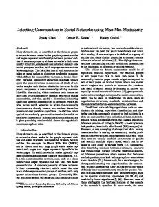
The regularization parameter τn is defined by (4.1), up to a constant, as a function of n, K, and the unobserved αn . Absorbing a constant factor into Cτ , we estimate αn by P i6=j Aij α ˆn = (5.3) n(n − 1)K and investigate the effect of the constant Cτ empirically. For this simulation, we generate networks with n = 500 or 2000 nodes with K = 3 communities. We consider two settings for θi ’s: (1) θi = 1 for all i (no hubs), and (2) P(θi = 1) = 0.8 and P(θi = 20) = 0.2 (20% hub nodes). We generate Z as follows: for 1 ≤ k1 < . . . < km ≤ K, we assign n · πk1 ···km nodes to the intersection of communities k1 , . . . , km , and for each node i in this set we set Zik = m−1/2 1(k ∈ {k1 , . . . , km }). Let π1 = π2 = π3 = π (1) , π12 = π13 = π23 = π (2) , π123 = π (3) and set (π (1) , π (2) , π (3) ) = (0.3, 0.03, 0.01). Finally, we choose αn so that the expected average node degree d¯ is either 20 or 40. We vary the constant factor Cτ in (4.1) in the range ˆ and Z to a binary {2−12 , 2−10 , . . . , 210 , 212 }. To use exNVI, we convert both the estimated Z overlapping community assignment by thresholding its elements at 1/K. The results, shown in Figure 5.1, indicate that the performance of OCCAM is stable over a wide range of the constant factor (2−12 − 25 ), and degrades only for very large values of Cτ . Based on this empirical evidence, we recommend setting α ˆ 0.2 K 1.5 τn = 0.1 n 0.3 . (5.4) n

10

(a) ρ = 0.1, n = 500

(b) ρ = 0.1, n = 2000

(c) ρ = 0.25, n = 500

(d) ρ = 0.25, n = 2000

Figure 1: Performance of OCCAM measured by exNVI as a function of Cτ .

11

5.2

Comparison to benchmark methods

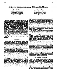
To compare OCCAM to other methods for overlapping community detection, we fix n = 500 and use the same settings for K, Z, θi ’s and αn as in Section 5.1. We set Bkk0 = ρ for k 6= k 0 , with ρ = 0, 0.05, 0.10, . . . , 0.5, and set (π (1) , π (2) , π (3) ) to be either (0.3, 0.03, 0.01) or (0.25, 0.07, 0.04). The regularization parameter τn is set to the recommended value (5.4), and detection performance is measured by exNVI. We compare OCCAM to both algorithmic methods and model-based methods that can be thought of as special cases of our model. Algorithmic methods we compare include the order statistics local optimization method (OSLOM) by Lancichinetti et al. (2011), the community overlap propagation algorithm (COPRA) by Gregory (2010), the nonnegative matrix factorization (NMF) on A computed via the algorithm of Gillis and Vavasis (2012), and the Bayesian nonnegative matrix factorization (BNMF) (Psorakis et al., 2011). Model-based methods we compare are two special cases of our model, the BKN overlapping community model (Ball et al., 2011) and the overlapping stochastic blockmodel (OSBM) (Latouche et al., 2009). For methods that produce continuous community membership values, thresholding was applied for the purpose of comparisons. For OCCAM and BNMF, where the membership vector is constrained to have norm 1, we use the threshold of 1/K; for NMF, where there are no such constraints to guide the choice of threshold, we simply use a small positive number 10−3 ; and for BKN, we follow the scheme suggested by the authors and assign node i to community k if the estimated number of edges between i and nodes in community k is greater than 1. For each parameter configuration, we repeat the experiment 200 times. Results are shown in Figure 5.2. As one might expect, all methods degrade as (1) the between-community edge probability approaches the within-community edge probability (i.e., ρ increases); (2) the overlap between communities increases; and (3) the average node degree decreases. In all cases, OCCAM performs best, but we should also keep in mind that the networks were generated from the OCCAM model. BKN and BNMF perform well when ρ is small but degrade much faster than OCCAM as ρ increases, possibly because they require shared community memberships for nodes to be able to connect, thus eliminating connections between pure nodes from different communities; NMF requires this too. OSLOM detects communities by locally modifying initial estimates, and when ρ increases beyond a certain threshold, the connections between pure nodes blur the “boundaries” between communities and lead OSLOM to assign all nodes to all communities. COPRA, a local voting algorithm, is highly sensitive to ρ for the same reasons as OSLOM, and additionally suffers from numerical instability that sometimes prevents convergence. OSBM performs well under the homogeneous node degree setting (when all θi = 1), where OSBM correctly specifies the data generating mechanism, but its performance degrades quickly in the presence of hubs. Overall, in this set of simulations OCCAM has a clear advantage over its less flexible competitors.

6

Application to SNAP ego-networks

The ego network datasets (McAuley and Leskovec, 2012) contain more than 1000 ego-networks from Facebook, Twitter and GooglePlus. In an ego network, all the nodes are friends of one central user, and the friendship groups or circles (depending on the platform) set by this user can be used as ground truth communities. This dataset was introduced by McAuley and Leskovec (2012), who also proposed an algorithm for overlapping community detection, which we will refer to as ML. We did not include this method in simulation studies because it uses additional node features 12

(a) A, d = 20, with hub nodes

(b) A, d = 40, with hub nodes

(c) B, d = 20, with hub nodes

(d) B, d = 40, with hub nodes

(e) A, d = 20, no hub node

(f) A, d = 40, no hub node

(g) B, d = 20, no hub node Figure 2: A:

(π (1) , π (2) , π (3) )

(h) B, d = 40, no hub node 13 = (0.3, 0.03, 0.03); B:(π (1) , π (2) , π (3) ) = (0.25, 0.07, 0.04)

which all other algorithms under comparison do not; however, we include it in comparisons in this section. Before comparing the methods, we carried out some pre-processing to make sure the test cases do in fact have a substantial community structure. First, we “cleaned” each network by (1) dropping nodes that are not assigned to any community; (2) dropping isolated nodes; (3) dropping communities whose pure nodes are less than 10% of the network size. Note that step (3) is done iteratively, i.e., after dropping the smallest community that does not meet this criterion, we inspect all remaining communities again and continue until either all communities meet the criterion or only one community remains. After this process is complete, we select cleaned networks that (a) contain at least 30 nodes; (b) have at least 2 communities; and (c) have Newman-Girvan modularities (Newman and Girvan, 2004) on the true communities of no less than 0.05, indicating some assortative community structure is present. These three rules eliminated 19, 45 and 28 networks respectively of the 132 GooglePlus networks, 455, 236 and 99 networks respectively out of 973 Twitter networks, and (b) eliminated 3 out of 10 Facebook networks. The remaining 40 GooglePlus networks, 183 Twitter networks, and 7 Facebook networks were used in all comparisons, using exNVI to measure performance. To get a better sense of what the different social networks look like and how different characteristics potentially P affect performance, we report the following summary statistics for each network: (1) density ij Aij /(n(n − 1)), i.e., the overall edge probability; (2) average node degree d; (3) the coefficient of variation of node degrees (the standard deviation divided by the mean) σd /d, which measures the amount of heterogeneity in the node degrees; (4) the proportion of overlapping nodes ro ; (5) Newman-Girvan modularity. Even though modularity was defined for non-overlapping communities, it still reflects the strength of the community structure in the networks in this dataset, which only have a modest amount of overlaps. We report the means and standard deviations of these measures for each of the social networks in Table 1. Note that Facebook and Gplus networks tend to be larger than Twitter networks, while Twitter networks tend to be denser, with more homogeneous degrees as reflected by σd /d, though their smaller size makes these measures less reliable. To compare methods, we report the average performance over each of the social platforms and the corresponding standard deviation in Table 2. We also report the mean pairwise difference between OCCAM and each of the other methods, along with its standard deviation in Table 3. Table 1: Mean (SD) of summary statistics for ego-networks #Networks n K Density d σd /d ro Modularity Facebook 7 224 3.3 0.137 28 0.644 0.030 0.418 (221) (0.8) (0.046) (29) (0.145) (0.021) (0.148) Gplus 40 414 2.3 0.170 53 1.035 0.057 0.171 (330) (0.5) (0.109) (34) (0.471) (0.077) (0.109) Twitter 183 62 2.8 0.264 15 0.595 0.036 0.204 (31) (0.9) (0.264) (8) (0.148) (0.055) (0.119)

As in simulation studies, we observe that OCCAM outperforms other methods. Gplus networks on average have the most heterogeneous node degrees and thus are challenging for COPRA and OSBM, while OCCAM is relatively robust to node degree heterogeneity. Further, Gplus networks tend to have higher proportions of overlapping nodes than Facebook networks; this creates difficulties for all methods. Empirically, we also found that OSLOM and COPRA are prone to 14

Table 2: Mean (SD) of exNVI for all methods. OCCAM OSLOM COPRA NMF BNMF BKN Facebook 0.576 0.212 0.394 0.314 0.500 0.474 (0.116) (0.068) (0.115) (0.079) (0.094) (0.107) Gplus 0.503 0.126 0.114 0.293 0.393 0.357 (0.038) (0.017) (0.036) (0.036) (0.046) (0.030) Twitter 0.451 0.208 0.232 0.212 0.437 0.346 (0.021) (0.012) (0.023) (0.013) (0.021) (0.017)

OSBM ML 0.473 0.133 (0.114) (0.033) 0.333 0.175 (0.039) (0.023) 0.348 0.200 (0.017) (0.010)

Table 3: Mean (SD) of pairwise differences in exNVI between OCCAM and other vs OSLOM vs COPRA vs NMF vs BNMF vs BKN vs OSBM Facebook 0.363 0.182 0.261 0.075 0.101 0.102 (0.093) (0.082) (0.071) (0.072) (0.053) (0.032) Gplus 0.377 0.389 0.210 0.110 0.146 0.171 (0.037) (0.037) (0.040) (0.038) (0.020) (0.028) Twitter 0.243 0.219 0.239 0.014 0.105 0.103 (0.020) (0.019) (0.016) (0.012) (0.012) (0.011)

methods. vs ML 0.443 (0.134) 0.328 (0.042) 0.251 (0.024)

convergence to degenerate community assignments, assigning all nodes to one community. NMF, BNMF and BKN often create substantial overlaps compared to other methods, likely because they do not allow connections between pure nodes from different communities. The results suggest that OCCAM works well when the overlap is not large even when modularity is relatively low, while other methods are more sensitive to modularity, which measures the strength of an assortative community structure. On the other hand, large overlaps between communities cause the performance of OCCAM to deteriorate, which is consistent with our theoretical results. ML is not readily comparable to others since it uses both network information and node features when fitting the model, and one would expect it do to better since it makes use of more information; however, using node features that are uncorrelated with the community structure can in fact worsen community detection, which may explain its poor performance on some of the networks. A fair comparison of computing times is difficult because the methods compared here are implemented in different languages. Qualitatively, we can say that the most expensive part of OCCAM is the K-medians clustering, which involves gradient descent, and is about one order of magnitude slower than NMF. The computational cost of OCCAM is comparable to that of BNMF, BKN and COPRA, and is at least two orders of magnitude less than that of OSLOM, OSBM and ML.

7

Discussion

This paper makes two major contributions, the model and the algorithm. The model we proposed for overlapping communities, OCCAM, is identifiable, interpretable, and flexible; it addresses limitations of several earlier approaches by allowing continuous community membership, allowing for pure nodes from different communities to be connected, and accommodating heterogeneous node degrees. Our goals in designing an algorithm to fit the model were scalability and of course accuracy, and therefore we made a number of modifications to spectral clustering to deal with the overlaps, most importantly replacing K-means with K-medians. Empirically we found the algorithm is a 15

lot faster than most of its competitors, and it performs well on both synthetic and real networks. We also showed estimation consistency under conditions that articulate the appropriate setting for our method – the overlaps are not too large and the network is not too sparse (the latter being a general condition for all community detection consistency, and the former specific to our method). In addition to its many advantages, our method has a number of limitations. The upper bound on the amount of overlap is a restriction, expressed by implicit condition B, which may not be easy to verify except in special cases. It is clear, however, that some limit on the amount of overlap is necessary for any model to be identifiable. Like all other spectral clustering based methods, OCCAM works best when communities have roughly similar sizes; this is implied by condition B which implicitly excludes communities of size o(n/K) as n and K grow. Further, our model only applies to assortative communities, in other words, requires the matrix of probabilities B to be positive definite. This constraint seems to be unavoidable if the model is to be identifiable. Like the vast majority of existing community detection methods, we assume that the number of communities K is given as input to the algorithm. There has been some very recent work on choosing K by hypothesis testing (Bickel and Sarkar, 2013) or a BIC-type criterion (Saldana et al., 2014) for the non-overlapping case; testing these methods and adapting them to the overlapping case is a topic for future work which is outside the scope of this manuscript but is an interesting topic. Another interesting and difficult challenge is detecting communities in the presence of “outliers” that do not belong to any community, considered by Zhao et al. (2011) and Cai and Li (2014). Our algorithm may be able to do this with additional regularization. Finally, incorporating node features when they are available into overlapping community detection is another challenging task for future, since the features may introduce both additional useful information and additional noise.

8

Appendix

8.1

Proof of identifiability

Proof of Theorem 2.1. We start with stating a Lemma of Tang et al. (2013): Lemma 8.1 (Lemma A.1 of Tang et al. (2013)). Let Y1 , Y2 ∈ Rn×d , d < n, be full rank matrices and G1 = Y1 Y1T , G2 = Y2 Y2T . Then there exists an orthonormal O such that p p √ dkG1 − G2 k( kG1 k + kG2 k) kY1 O −2 kF ≤ (8.1) λmin (G2 ) where λmin (·) i sthe smallest positive eigenvalue. Lemma 8.1 immediately implies Claim 1. For two full rank matrices H1 , H2 ∈ Rn×K satisfying H1 H1T = H2 H2T , there exists an orthonormal matrix OH such that H1 OH = H2 . Suppose parameters (αn,1 , Θ1 , Z1 , B1 ) and (αn,2 , Θ2 , Z2 , B2 ) generate the same W . Then by Lemma 1, there exists an orthonormal matrix O12 such that 1/2

1/2

αn,1 Θ1 Z1 B1 O12 = αn,2 Θ2 Z2 B2

16

(8.2)

We then show that the indices for “pure” rows in Z1 and Z2 match up. More precisely, for 1 ≤ k ≤ K, let Ik := {i : rowi (Z1 ) = ek }. We show that rowj (Z2 ), j ∈ I k are also pure nodes, i.e., there exists k 0 such that {j : rowj (Z2 ) = ek0 } = I k . It suffices to show that there exists i ∈ I k such that rowi (Z2 ) is pure, then the claim follows from the fact that all rows in Z2 with indices in Ik equal each other, since their counterparts in Z1 are equal. We prove this by contradiction: if {rowi (Z2 ), i ∈ I k } are not pure nodes, then for any i ∈ I k , there exists {i1 , . . . , iK } ⊂ {1, . . . , n} − I k and ω1 , . . . , ωK ≥ 0 such that rowi (Z2 ) =

K X

ωk rowik (Z2 )

(8.3)

k=1

By (8.2), this yields rowi (Z1 ) =

K X

ωk

k=1

αn,1 (Θ1 )ik ik rowik (Z1 ) αn,2 (Θ2 )ik ik

(8.4)

i.e. the ith row of Z1 can be expressed as a non-negative linear combination of at most K rows outside I k , and thus rowi (Z1 ) is not pure. Essentially we have shown the identifiability for all pure nodes. To show identifiability for the rest, take one pure node from each community as ˜ := {j1 , . . . , jK }, where jk ∈ I k , 1 ≤ k ≤ K. Let Z K be the submatrix representative, i.e., let I 1 ˜ similarly define Z K , and let Θ ˜ 1 and Θ ˜ 2 be induced by concatenating rows of Z1 with indices in I, 2 K K the corresponding submatrices of Θ1 and Θ2 . Note Z1 and Z2 are both order K permutations, which is an ambiguity allowed by our definition of identifiability, so we take Z1K = Z2K = I. By (8.2), ˜ 1 B 1/2 O12 = αn,2 Θ ˜ 2 B 1/2 . αn,1 Θ (8.5) 1 2 1/2 1/2 ˜ 1 )kk = krowk (αn,1 ΘK B 1/2 O12 )k2 = By condition I1, both B1 O12 and B2 have rows of norm 1, so αn,1 ·(Θ 1 1 1/2 ˜ ˜ ˜ B )k = α · ( Θ ) and therefore α Θ = α Θ . Then from (8.5) we have krowk (αn,2 ΘK 2 n,1 2 kk n,1 1 n,2 2 2 2 1/2

1/2

B1 O12 = B2 1/2

(8.6)

1/2

Thus B1 = B1 O12 (B1 O12 )T = B2 , and (8.2) implies αn,1 Θ1 = αn,2 Θ2 since all rows of Z1 and Z2 are normalized. This in turn implies αn,1 = αn,2 by condition I3 and thus Θ1 = Θ2 . Finally, plugging all of this back into (8.2) we have Z1 = Z2 .

8.2

Proof of consistency

ˆ follows the steps of the algorithm: we first bound Proof outline: The proof of consistency of Z ∗ ˆ the difference between Xτn and the row-normalized version of the true node positions X ∗ with high probability (Lemma 8.2); then bound the difference between Sˆ and the true community centers S = B 1/2 (Lemma 8.3) with high probability; these combine to give a bound on the difference ˆ and Z (Theorem 4.1). between Z Lemma 8.2. Assume conditions A1, A2 and A3 hold. When

log n nαn

1.5 α0.2 n K , n0.3

→ 0 and K = O(log n), there

for large enough n, we have exists a global constant C1 , such that with the choice τn = ! 4 ˆ ∗ O ˆ − X ∗ kF kX C1 K 5 τn X √ P ≤ ≥ 1 − P1 (n, αn , K) (8.7) 1 n (nαn ) 5 17

ˆ where P1 (n, αn , K) → 0 as n → ∞, and OXˆ is an orthonormal matrix depending on X. ˆ τ∗ as Xτ∗ ∈ Rn×K , where rowi (Xτ∗ ) := Proof of Lemma 8.2. Define the population version of X n n n Xi· ˆ τ∗ O ˆ − Xτ∗ kF for a certain orthonormal matrix O ˆ and then the . We first bound k X n n X X kXi· k2 +τ bias term kXτ∗n − X ∗ kF . Then the triangular inequality gives (8.7). ˆ τ∗ O ˆ − Xτ∗ kF . For any orthonormal matrix O, We now bound kX n n X ˆ ∗ O − X ∗ )k2 = krowi (X ˆ ∗ )O − rowi (X ∗ )k2 krowi (X τn τn τn τn

X

ˆ ˆ Xi· O Xi· Xi·



i· O = = − −

ˆ ˆ kX k + τ kX k + τ 2 i· 2 n i· 2 n 2 kXi· k2 + τn kXi· Ok2 + τn ˆ i· O(kXi· k2 − kX ˆ i· Ok2 ) + kX ˆ i· Ok2 (X ˆ i· O − Xi· ) + τn (X ˆ i· O − Xi· )k2 kX = ˆ i· Ok2 + τn )(kXi· k2 + τn ) (kX ˆ i· Ok2 + τn )kX ˆ i· O − Xi· k2 ˆ i· O − Xi· k2 ˆ i· O − Xi· k2 (2kX 2kX 2kX ≤ ≤ ≤ . ˆ i· Ok2 + τn )(kXi· k2 + τn ) kXi· k2 + τn τn (kX Then ˆ∗ O ˆ kX τn X

v u n  2 ˆ uX 2 ∗ ˆ i· O ˆ − Xi· k2 = 2kXOXˆ − XkF . − Xτn kF ≤ t kX 2 X τn τn i=1

By Lemma 8.1, there exists an orthonormal matrix OXˆ , such that q  p √ T T T T ˆ ˆ ˆ ˆ 2 KkX X − XX k kX X k + kXX k ˆ ∗ O ˆ − X ∗ kF ≤ kX τn X τn τn λmin (XX T ) q  p √ T T T T T ˆ ˆ ˆ ˆ 2 KkX X − XX k kX X − XX k + 2 kXX k ≤ τn λmin (XX T ) p  p √ 2 KkA − W k kA − W k + 2 kW k = τn λmin (W )

(8.8)

where k · k denotes the operator norm. We then bound each term on the RHS of (8.8). To bound kA − W k, we mostly follow Tang et al. (2013). Let U and U be n × K matrices of the ˆU ˆ T and P W := U U T , then leading K eigenvectors of A and W respectively, and define P A := U T T W = XX = P W XX P W = P W W P W , and similarly A = P A AP A . We have kA − W k =kP A AP A − P W W P W k ≤kP A (A − W )P A k + k(P A − P W )W P A k + kP A W (P A − P W )k + k(P A − P W )W (P A − P W )k ≤kA − W k + 2kP A − P W kkW k + kP A − P W k2 kW k .

(8.9)

By Appendix A.1 of Lei and Rinaldo (2013), we have √ 2 2KkA − W k . kP A − P W k ≤ kP A − P W kF ≤ λmin (W ) 18

(8.10)

By Theorem 5.2 of Lei and Rinaldo (2013), when log n/(nαn ) → 0 and θi ’s are uniformly bounded by a constant Mθ , there exists constant Cr,Mθ depending on r, such that with probability 1 − n−r √ kA − W k ≤ Cr nαn . (8.11) Since Mθ is a global constant in our setting, we write Cr := Cr,Mθ . ˆ τ∗ O ˆ − Xτ∗ kF , it remains to bound the maximum and minimum eigenIn order to bound kX n n X T Z ]B, values of W . We will show that the eigenvalues of (nαn )−1 W converge to those of E[θ12 Z1· 1· which is strictly positive definite: for any v ∈ RK , v

T

T E[Z1· Z1· ]

≥

K X

P(1 ∈ Ck ) · v T ek eTk v ≥ 0 ,

k=1

where Ck denotes the set of nodes in community k and ek denotes the vector the kth element equal to 1 and all others being 0. Equality holds only when all v T ek eTk v = vk2 = 0, i.e. v = 0. Claim 2. Assume that θi > 0 for all i, and both Z and B are full rank. Let λ0 and λ1 denote the T Z ]B. Then smallest and largest eigenvalues of E[θ12 Z1· 1· !   1 2 n λ (W ) max 2 √ P − λ1 >  ≤ 2K 2 exp − 4 (8.12) nαn Mθ K 3 + 13 Mθ2 K K !   1 2 λmin (W ) 2 2 n √ P − λ0 >  ≤ 2K exp − 4 (8.13) nαn Mθ K 3 + 13 Mθ2 K K Proof of Claim 2. For k = 1, . . . , K, let λk denote the kth largest eigenvalue of W , then !     W B 1/2 Z T Θ2 ZB 1/2 ΘZBZ T Θ λk = λk = λk nαn n n !   T 2 n 1X 2 T Z Θ ZB = λk = λk θi Zi· Zi· B n n i=1

XX T

where the second equality is due to the fact that and X T X share the same K leading √ eigenvalues (X = αn ΘZB 1/2 ). The third equality holds because B 1/2 is full rank. To show (8.13), it suffices to show that ! ! n

1 X

1 2

2 T 2 T 2 n √ P (8.14) θi Zi· Zi· B − E[θ1 Z1· Z1· B] >  ≤ 2 exp − 4 n Mθ K 3 + 31 Mθ2 K K i=1 √ For any k, l ∈ {1, . . . , K}, {θi2 (Zi·T Zi· B)kl }i are an iid sequence uniformly bounded by Mθ2 K with
mean E[θi2 (Zi·T Zi· B)] kl . By Bernstein’s inequality, ! ! ! n 1X 1 2 n T 2 √ P θi2 Zi·T Zi· B − E[θ12 Z1· Z1· B] . >  ≤ 2 exp − 4 1 2 n M K + θ 3 Mθ K i=1 kl

By the union bound and kAk ≤ kAkF , we have ! ! n

1 X

1 2 n

T 2 √ P θi2 Zi·T Zi· B − E[θ12 Z1· Z1· B] > K ≤ 2K 2 exp − 4 . 1 2 n M K + θ 3 Mθ K i=1 Replacing  by /K completes the proof of Claim 2. 19

ˆ τ∗ O ˆ −Xτ∗ kF . Taking We now return to the proof of Lemma 8.2 and complete the bound on kX n n X  to be λ21 and λ20 respectively in (8.12) and (8.13), by Claim 2, kW k ≤ 23 nαn λ1 ≤ 32 Mλ1 nαn K and λmin (W ) ≥ 12 nαn λ0 ≥ 21 Mλ0 nα hold with probability: ! ! 1 1 2 2 nλ nλ 0 1 8 8 √ √ + 2K 2 exp − 4 1 − 2K 2 exp − 4 Mθ K 3 + 16 Mθ2 K Kλ0 Mθ K 3 + 61 Mθ2 K Kλ1 ! 2 1 nM λ ≥1 − 4K 2 exp − 4 5 8 1 20 5/2 Mθ K + 6 Mθ K Mλ0 Plugging this, together with (8.10) and (8.10), back into (8.9), we have ! √ 4 2KkW k 8KkA − W kkW k ˆX ˆ T − XX T k ≤ kA − W k 1 + kX + λmin (W ) (λmin (W ))2 ! √ √ 12 2KMλ1 48K 2 Cr Mλ1 + (8.15) ≤ Cr nαn 1 + √ Mλ 0 Mλ0 2 nαn   1 nMλ0 2 2 8 with probability at least 1 − 4K exp − M 4 K 5 + 1 M 2 K 5/2 M − n−r . Then plugging (8.15) and θ

6

θ

λ0

Claim 2 into (8.8), we have ˆ ∗ O ˆ − X ∗ kF kX τn X τn √

≤

2 K τn

√ 2 K ≤ τn "

ˆX ˆ T − XX T k kX  √ Cr nαn 1 +

q  p T T T ˆ ˆ kX X − XX k + 2 kXX k

λmin (XX T )  √ 48K 2 Cr Mλ1 12 2KKMλ1 + Mλ √nαn Mλ0 0 M

λ0 nαn 2K  !# 1 √ 2 2C M p √ 2KKM 12 48K r λ1 λ1 + 6Mλ1 nαn  ·  Cr nαn 1 + + √ Mλ0 Mλ0 nαn ! √ √ √ 4Cr K 12 2Mλ1 K K 48Cr Mλ1 K 2 = + 1+ √ τn Mλ0 Mλ 0 Mλ0 2 nαn  " !# 1 √ √ 2 2 p 12 2Mλ1 K K 48Cr Mλ1 K 1 ·  Cr √ + + + 6Mλ1  √ nαn M λ0 nαn Mλ0 2 nαn 3

(8.16)

K By assumption K = O(log(n)), we have nα → 0, thus for large enough n, the following n inequalities that simplify (8.16) hold: √ √ (24 − 12 2)Mλ1 K K 48Cr Mλ1 K 2 −1≥ √ Mλ 0 Mλ0 2 nαn !# 1 " √ √ 2 √ p 1 12 2Mλ1 K K 48Cr Mλ1 K 2 (3 − 6) Mλ1 ≥ Cr √ + + , √ nαn M λ0 nαn Mλ0 2 nαn

20

and we have

K2 RHS of (8.16) ≤ C˜r · τn 288Cr Mλ1 3/2 , which Mλ0 2 ˆ τ∗ O ˆ − Xτ∗ kF . kX n n X

where the constant C˜r :=

(8.17)

for simplicity we will continue to write as Cr . This

completes the bound on The second part of the proof requires a bound on kXτ∗n − X ∗ kF . From the defintion of Xτ∗n , we can write 2 √ n  X τn / αn kXτ∗n − X ∗ k2F = . (8.18) √ √ kXi· k2 / αn + τn / αn i=1

q p √ k √ · 2 = θi kZi· B 1/2 k2 = θi Zi· BZ T ≥ θi λmin (B) ≥ θi mB > 0, by assumption, for Since kX i· αn   √ k √ i· 2 <  mB ≤ P(θi < ) ≤ Cθ . Therefore, for any  ∈ (0, 0 ), we have  ∈ (0, 0 ), we have P kX αn " E

2 #  2 √ √ τn / αn τn / αn ≤ Cθ  + (1 − Cθ ) √ √ √ √ kXi· k2 / αn + τn / αn  mB + τn / αn

(8.19)

√ √ 3/2 By assumption, τn / αn → 0, so for large enough n such that τn / αn < 0 , taking  := √ 2/3 (τn / n) < 0 , we have √ √ LHS of (8.19) ≤ Cθ (τn / αn )2/3 + (1 − Cθ (τn / αn )2/3 )

!2 √ (τn / αn )1/3 √ mB + (τn / αn )1/3


√ 2/3 ≤ Cθ + m−1 B (τn / αn ) Then for any δ > 0, we have   kXτ∗n − X ∗ k2F √ 2/3 )(τ / α ) > δ − (Cθ + m−1 P n n B n !     1 2 δ n kXτ∗n − X ∗ k2F kXτ∗n − X ∗ k2F ≤P −E > δ ≤ exp − 2 1 n n 1 + 3δ

(8.20)

where the second inequality is Bernstein’s inequality plus the fact that each summand
in the numer√ 2/3 . ator of (8.18) is uniformly bounded by 1 with an expectation bounded by Cθ + m−1 B (τn / αn ) We can now complete the proof of Lemma 8.2. Combining (8.17) and (8.20) yields ! ˆ ∗ O ˆ − X ∗ kF kX √ Cr K 2 τn X −1 2/3 √ P ≤ √ + δ + (Cθ + mB )(τn / αn ) n τn n ≥1 − P1 (n, αn , K; r)

(8.21) 0.2

1.5

K The optimal τn that minimizes the RHS of the inequality inside the probability is τn = αnn0.3 – here for simplicity we drop the constant factor in τn , the effect of which we evaluated em1 pirically in Section 5. Plugging this into (8.21) and taking δ = K(nαn )− 5 and denote C1 :=

21



2 3 (Cθ

2

+

−1 mB )Cr3

− 2 exp −

3 5

   2 1 3 Mλ0 2 n 5 −r −4 exp − 8 2 +1+ 23 Cr (Cθ + m−1 and P (n, α , K; r) := n ) 1 n 5 B Mθ4 K 5 + 16 Mθ2 Mλ0 K 2 ! 2

8 3 − 1 K 5 n 5 αn 5 2 1 4 1+ 13 K 3 (nαn ) 5

, we obtain Lemma 8.2. Note that since we are free to choose and fix r,

we can drop the dependence on it from P1 , as we did in the statement of Lemma 8.2. The next step is to show the convergence of the estimated cluster centers Sˆ to the population cluster centers SF . Lemma 8.3. Recall that F denotes the popualtion distribution of the rows of X ∗ and let Sˆ ∈ ˆ ∗ ; S) and SF ∈ arg minS L(F; S). Assume that conditions A1, A2, A3 and B hold. arg minS Ln (X τn log n Then if nαn → 0 and K = O(log n), for large enough n we have 9

ˆ ˆ ; SF ) ≤ P DH (SO X

C2 K 5

1

(nαn ) 5

! ≤ 1 − P1 (n, αn , K) − P2 (n, αn , K)

(8.22)

where C2 is a global constant, P2 (n, αn , K) → 0 as n → ∞ and DH (·, ·) is as defined in condition B. ˆ ∗ and X ∗ have l2 norms bounded by 1, the sample space Proof of Lemma 8.3. Since the rows of X τn of F is uniformly bounded in the unit l2 ball. Following the argument of Pollard et al. (1981), we show that all cluster centers estimated by K-medians fall in the l2 ball centered at origin with radius 3, which we denote as R. Otherwise, if there exists an estimated cluster center s outside R, it is at least distance 2 away from any point assigned to its cluster. Therefore, moving s to an arbitrary point inside the unit ball yields an improvement in the loss function since any two points inside the unit ball are at most distance 2 away from each other. ˆ τ∗ O ˆ ; S) to L(F; S) and then show the optimum We first show the uniform convergence of Ln (X n X ˆ ˆ := arg minS Ln (X ˆ τ∗ O ˆ ; S) is close to that of L(F; S). Let SO ˆ τ∗ O ˆ ; S). We start with of Ln (X n n X X X showing that ˆ ∗ ˆ − X ∗ kF X ˆ ∗ O ˆ ; S) − Ln (X ∗ ; S)| ≤ kXτn O√ sup |Ln (X . (8.23) τn X n S⊂R To prove (8.23), take any s ∈ R. For each i, let sˆ and s be (possibly identical) rows in S that are ˆ ∗ O ˆ )i· and X ∗ respectively in l2 norm. We have closest to (X τn X i· ˆ ∗ O ˆ )i· − sˆk2 ≤ k(X ˆ ∗ O ˆ )i· − X ∗ k2 kXi·∗ − sk2 − k(X τn X τn X i· ˆ ∗ O ˆ )i· k2 . Thus |k(X ˆ ∗ O ˆ )i· − sˆk2 − ˆ ∗ O ˆ )i· − sˆk2 − kX ∗ − sk2 ≤ kX ∗ − (X and similarly, k(X τn X τn X τn X i· i· ˆ ∗ O ˆ )i· − X ∗ k2 . Combining this inequalities for all rows, we have kXi·∗ − sk2 | ≤ k(X τn X i· n  1 X  ∗ ∗ ˆ ˆ ∗ O ˆ )i· − sˆk2 − kX ∗ − sk2 |Ln (Xτn OXˆ ; S) − Ln (X ; S)| = k(X τn X i· n i=1 v u n u1 X ˆ ∗ O ˆ )i· − X ∗ k2 = √1 kX ˆ ∗ O ˆ − X ∗ kF . ≤t k(X τn X τn X i· 2 n n i=1

22

(8.24)

Then since that (8.24) holds for any S, the uniform bound (8.23) follows. For simplicity, we introduce the notation “S ⊂ R”, by which we mean that the rows of a matrix S belong to the set R. We now derive the bound for supS⊂R |Ln (X ∗ ; S)−L(F; S)|, which, without taking the supremum, is easily bounded by Bernstein’s inequality. To tackle the uniform bound, we employ an -net (see, for example, Haussler and Welzl (1986)). There exists an -net R , with size |R | ≤ CR K log K , where CR is a global constant. For any S˜ ⊂ R , S˜ ∈ RK×K , notice that ˜ for min1≤k≤K kXi·∗ − S˜k· k2 is a random variable uniformly bounded by 6 with expectation L(F; S) each i. Therefore, by Bernstein’s inequality, for any δ > 0 we have !   1 2 nδ nδ 2 ∗ ˜ 2 ˜ (8.25) = exp − P(|Ln (X ; S) − L(F; S)| > δ) ≤ exp − 2 72 + 4δ 4RM + 32 RM δ The number of all such S˜ ⊂ R is bounded by     K K K K K ˜ ˜ log C R   ≤ CR log {S : S ⊂ R } = K   By the union bound, we have P

˜ − L(F; S) ˜ > δ sup L(X ∗ ; S)

˜ S∈R 

!

    K K K nδ 2 < CR log exp −   72 + 4δ

(8.26)

The above shows the uniform convergence of the loss functions for S˜ from the -net R . We ˜ ⊂ R , such then expand it to the uniform convergence of all S ⊂ R. For any S ⊂ R, there exists S ˜ ˜ that both Ln (·; S) and L(·; S) can be well approximated by Ln (·; S) and L(·; S) respectively. To ˜ = S(S). ˜ emphasize the dependence of S˜ on S, we write S Formally, we now prove the following. ˜ sup |Ln (X ∗ ; S) − Ln (X ∗ ; S(S))|