Overlapping Communities in Social Networks ... - Semantic Scholar

Overlapping Communities in Social Networks∗ arXiv:1412.4973v2 [cs.SI] 18 Dec 2014

Jan Dreier, Philipp Kuinke, Rafael Przybylski, Felix Reidl, Peter Rossmanith, and Somnath Sikdar Theoretical Computer Science RWTH Aachen University, 52074 Aachen, Germany

Abstract Complex networks can be typically broken down into groups or modules. Discovering this “community structure” is an important step in studying the large-scale structure of networks. Many algorithms have been proposed for community detection and benchmarks have been created to evaluate their performance. Typically algorithms for community detection either partition the graph (nonoverlapping communities) or find node covers (overlapping communities). In this paper, we propose a particularly simple semi-supervised learning algorithm for finding out communities. In essence, given the community information of a small number of “seed nodes”, the method uses random walks from the seed nodes to uncover the community information of the whole network. The algorithm runs in time O(k · m · log n), where m is the number of edges; n the number of links; and k the number of communities in the network. In sparse networks with m = O(n) and a constant number of communities, this running time is almost linear in the size of the network. Another important feature of our algorithm is that it can be used for either non-overlapping or overlapping communities. We test our algorithm using the LFR benchmark created by Lancichinetti, Fortunato, and Radicchi [15] specifically for the purpose of evaluating such algorithms. Our algorithm can compete with the best of algorithms for both non-overlapping and overlapping communities as found in the comprehensive study of Lancichinetti and Fortunato [13]. ∗

Research funded by DFG Project RO 927/13-1 “Pragmatic Parameterized Algorithms.”

1

1

Introduction

Many real-world graphs that model complex systems exhibit an organization into subgraphs, or communities that are more densely connected on the inside than between each other. Social networks such as Facebook and LinkedIn divide into groups of friends or coworkers, or business partners; scientific collaboration networks divide themselves into research communities; the World Wide Web divides into groups of related webpages. The nature and number of communities provide a useful insight into the structure and organization of networks. Discovering the community structure of networks is an important problem in network science and is the subject of intensive research [7, 17, 3, 20, 5, 19, 18, 1, 22, 21]. Existing community detection algorithms are distinguished by whether they find partitions of the node set (non-overlapping communities) or node covers (overlapping communities). Typically finding overlapping communities is a much harder problem and most of the earlier community detection algorithms focused on finding disjoint communities. A comparative analysis of several community detection algorithms (both non-overlapping and overlapping) was presented by Lancichinetti and Fortunato in [13]. In this paper we closely follow their test framework, also called the LFR-benchmark. The notion of a community is a loose one and currently there is no well-accepted definition of this concept. A typical approach is to define an objective function on the partitions of the node set of the network in terms of two sets of edge densities: the density of the edges within a partite set (intra-community edges) and the density of edges across partitions (inter-community edges). The “correct” partition is the one that maximizes this function. Various community detection algorithms formalize this informal idea differently. One of the very first algorithms by Girvan and Newman [7] introduced a measure known as modularity which, given a partition of the nodes of the network, compares the fraction of inter-community edges with the edges that would be present had they been rewired randomly preserving the node degrees. Other authors such as Palla et al. [19] declare communities as node sets that formed by overlapping maximal cliques. Rosvall and Bergstrom [22] define the goodness of a partition in terms of the number of bits required to describe per step of an infinite random walk in the network, the intuition being that in a “correct” partition, a random walker is likely to spend more time within communities rather than between communities, thereby decreasing the description of the walk. A severe restriction of many existing community detection algorithms is that they are too slow. Algorithms that optimize modularity typically take O(n2 ), even on sparse networks. The overlapping clique finding algorithm of Palla et al. [19] take exponential time in the worst case. In other cases, derivation of worst-case running time bounds are ignored. 2

Our contribution. Given that it is unlikely that users of community detection algorithms would unanimously settle on one definition of what constitutes a community, we feel that existing approaches ignore the user perspective. To this end, we chose to design an algorithm that takes the network structure as well as user preferences into account. The user is expected to classify a small set of nodes of the network into communities (which may be 6–8% of the nodes of each community). Obviously this is possible only when the user has some information about the network, such as its semantics, which nodes are important and into which communities they are classified. Such situations are actually quite common. The user might have data only on the leading scientific authors in a co-authorship network and would like to find out the research areas of the remaining members of the network. He may either be interested in a broad partition of the network into into its main fields or a fine grained decomposition into various subfields. By labeling the known authors accordingly, the user can specify which kind of partition he is interested in. Another example would be the detection of trends in a social network. Consider the case where one knows the political affiliations of some people and aims to discover political spectrum of the whole network, for example, to predict the outcome of an election. Another scenario where this may be applicable is in recommendation systems. One might know the preferences of some of the users of an online retail merchant possibly because they purchase items much more frequently than others. One could then use this in the network whose nodes consist of users, with two nodes connected by an edge if they represent users that had purchased similar products in the past. The idea now would be to use the knowledge of the preferences of a few to predict the preferences of everyone in the network. An important characteristic of algorithms surveyed in [13] is that the algorithms either find disjoint communities or overlapping ones. Most algorithms solve the easier problem of finding disjoint communities. The ones that are designed to find overlapping communities such as the overlapping clique finding algorithm of Palla et al. [19] do not seem to yield very good results (see [13]). Our algorithm naturally extends to the overlapping case. Of course, there is a higher price that has to be paid in that the number of nodes that need to be classified by the user typically is larger (5% to 10% of the nodes per community). The algorithm, however, does not need any major changes and we view this is as an aesthetically pleasing feature of our approach. Thirdly, in many other approaches, the worst-case running time of the algorithms is neither stated nor analyzed. We show that our algorithm runs in time O(k · m · log n), where k is the number of communities to be discovered (which is supplied by the user), n and m are the number of nodes and edges in the network. In the case of sparse graphs and a constant number of communities, the running time is O(n · log n). Given that even an O(n2 ) time algorithm is too computationally expensive on many real world 3

graphs, a nearly linear time algorithm often is the only feasible solution. Finally, we provide an extensive experimental evaluation of our algorithm on the LFR benchmark. In order to ensure a fair comparison with other algorithms reviewed in [13], we choose all parameters of the benchmark as in the original paper. This paper is organized as follows. In Section 2, we review some of the more influential algorithms in community detection. In Section 3, we describe our algorithm and analyze its running time. In Sections 4 and 5, we present our experimental results. Finally we conclude in Section 6 with possibilities of how our approach might be extended.

2

The Major Algorithms

In what follows, we briefly describe some common algorithms for community detection. We are particularly interested in the performance of these algorithms as reported in the study by Lancichinetti and Fortunato [13] on their LFR benchmark graphs. The Girvan-Newman algorithm. One of the very first algorithms for detecting disjoint communities was invented by Girvan and Newman [7, 17]. Their algorithm takes a network and iteratively removes edges based on a metric called edge betweenness. The betweenness of an edge is defined as the number of shortest paths between vertex pairs that pass through that edge. After an edge is removed, betweenness scores are recalculated and an edge with maximal score is deleted. This procedure ends when the modularity of the resulting partition reaches a maximum. Modularity is a measure that estimates the quality of a partition by comparing the network with a so-called “null model” in which edges are rewired at random between the nodes of the network while each node keeps its original degree. Formally, the modularity of a partition is defined as: 1 X di dj Q= Aij − 2m i,j 2m

!

δ(i, j),

(1)

where Aij represent the entries of the adjacency matrix of the network; di is the degree of node i; m is the number of edges in the network; and δ(i, j) = 1 if nodes i and j belong to the same set of the partition and 0 otherwise. The term di dj /2m represents the expected number of edges between nodes i and j if we consider a random model in which each node i has di “stubs” and we are allowed to connect stubs at random to form edges. This is the null model against which the within-community edges of the partition is compared against. The worst-case complexity of the Newman-Girvan algorithm is dominated by the time taken to compute the betweenness scores and is O(mn) for general graphs and O(n2 ) for sparse graphs [2]. 4

The greedy algorithm for modularity optimization by Clauset et al.[3]. This algorithm starts with each node being the sole member of a community of one, and repeatedly joins two communities whose amalgamation produces the largest increase in modularity. The algorithm makes use of efficient data structures and has a running time of O(m log2 n), which for sparse graphs works out to O(n log2 n). Fast Modularity Optimization by Blondel et al. The algorithm of Blondel et al. [1] consists of two phases which are repeated iteratively. It starts out by placing each node in its own community and then locally optimizing the modularity in the neighborhood of each node. In the second phase, a new network is built whose nodes are the communities found out in the first phase. That is, communities are replaced by “super-nodes”; the within-community edges are modeled by a (weighted) self-loop to the super-node; and the between-community edges are modeled by a single edge between the corresponding super-nodes, with the weight being the sum of the weights of the edges between these two communities. Once the second phase is complete, the entire procedure is repeated until the modularity does not increase any further. The algorithm is efficient due to the fact that one can quickly compute the change in modularity obtained by moving an isolated node into a community. Lancichinetti and Fortunato opine that modularity-based methods in general have a rather poor performance, which worsens for larger networks. The algorithm due to Blondel et al. performs well probably due to the fact that the estimated modularity is not a good approximation of the real one [13]. The CFinder algorithm of Palla et al. One of the first algorithms that dealt with overlapping communities was proposed by Palla et al. [19]. They define a community to be a set of nodes that are the union of k-cliques such that any one clique can be reached from another via a series of adjacent k-cliques. Two k-cliques are defined to be adjacent if they share k − 1 nodes. The algorithm first finds out all maximal cliques in the graph, which takes exponentialtime in the worst case. It then creates a symmetric clique-clique overlap matrix C which is a square matrix whose rows and columns are indexed by the set of maximal cliques in the graph and whose (i, j)th entry is the number of vertices that are in both the ith and j th clique. This matrix is then modified into a binary matrix by replacing all those entries with value less than k − 1 by a 0 and the remaining entries by a 1. The final step is to find the connected components of the graph represented by this binary symmetric matrix which the algorithm reports as the communities of the network. The authors report to have tested the algorithm on various networks including

5

the protein-protein interaction network of Saccharomyces cerevisiae 1 with k = 4; the co-authorship network of the Los Alamos condensed matter archive (with k = 6). Lancichinetti and Fortunato report that CFinder did not perform particularly well on the LFR benchmark and that its performance is sensitive to the sizes of community (but not the network size). For networks will small communities it has a decent performance, but has a worse performance on those with larger communities. Using random walks to model information flow. Rosvall and Bergman [22] approach the problem of finding communities from an information-theoretic angle. They transform the problem into one of finding an optimal description of an infinite random walk in the network. Given a fixed partition M of n nodes into k clusters, Rosvall and Bergman use a two-level code where each cluster is assigned a unique codeword and each node is assigned a codeword which is unique per community. One can now define the average number of bits per step that it takes to describe an infinite random walk on the network partitioned according to M . The intuition is that a random walker is statistically likely to spend more time within clusters than between clusters and therefore the “best” partition corresponds to the one which has the shortest possible description. An approximation of the best partition is found out using a combination of a greedy search heuristic followed by simulated annealing. Lancichinetti and Fortunato report that this algorithm (dubbed Infomap) was the best-performing among all other community detection algorithms on their benchmark.

3

The Algorithm

We assume that the complex networks that we deal with are modeled as connected, undirected graphs. The algorithm receives as input a network and a set of nodes such that there is at least one node from each community that we are aiming to discover. These nodes are called seed nodes and it is possible that a particular seed node belongs to multiple communities. The affinity of a node in the network to a community is 1 if it belongs to it; if it does not belong to it, it has an affinity of 0. We allow intermediate affinity values and view these as specifying a partial belonging. The user specifies the affinities of the seed nodes for each of the communities. For all other nodes, called non-seed nodes, we want deduce the affinity to each community using the information given by the seed nodes’ 1

A species of yeast used in wine-making, baking, and brewing.

6

affinities and the network structure. The main idea is that non-seed nodes should adopt the affinities of seed nodes within their close proximity. We define a proximity measure based on random walks: Each random walk starts at a non-seed node, traverses through the graph, and ends as soon as it reaches a seed node. The affinity of a non-seed node u for a given community is then the weighted sum of the affinities of the seed nodes for that community and reachable by a random walk starting at u, the weights being the probabilities that a random walk from u ends up at a certain seed node. Each step of a random walk can be represented as the iterated product of a transition matrix P . The result of the (infinite) walk itself can be expressed as limk→∞ P k . One of the contributions of this paper is to show how the calculation of these limits can be reduced to solving a symmetric, diagonally dominant system of linear equations (with different right-hand-sides per community), which can be done in O(m log n) time, where m is the number of edges in the graph. The fact that such systems can be solved in almost linear time was discovered by Spielman and Teng [23, 6, 24, 11, 12, 25]. If we assume that our networks are sparse in the sense that m = O(n), the running time of our algorithm can be bounded by O(n log n).

3.1

Absorbing Markov Chains and Random Walks

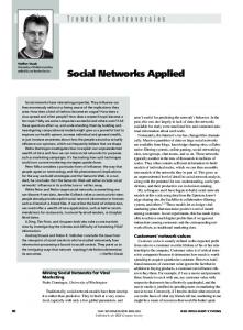
We now provide a formal description of our model. The input is an undirected, connected graph G = (V, E) with nodes v1 , . . . , vn , m edges and a nonempty set of s seed nodes. We also know that there are k (possibly overlapping) communities which we want to discover. The community information of a node v is represented by a 1 × k vector called the affinity vector of v, denoted by B(v) = (α(v, 1), . . . , α(v, k))T . The entry α(v, l) of the affinity vector represents the affinity of node v to community l. It may be interpreted as the probability that a node belongs to this community. We P point out that ki=1 α(v, l) need not be 1. An example of this situation is when v belongs to multiple communities with probability 1. The user-chosen affinity vectors of all seed nodes are part of the input. The objective is to derive the affinity vectors of all non-seed nodes. Since we require the random walks to end as soon as they reach a seed node, we transform the undirected graph G into a directed graph G0 as follows: replace each undirected edge {u, v} by arcs (u, v) and (v, u); then for each seed node, remove its outarcs and add a self-loop. This procedure is illustrated in Figure 1.

7

x1

x2 (a) Example graph with seed nodes x1 , x2 .

x1

x2

(b) Example graph with seed nodes x1 , x2 after transformation. Figure 1: Remove outgoing edges and add self-loop for all seed nodes in an example graph. A random walk reaching x1 or x2 will stay there forever.

. Random walks in this graph can be modelled by an n × n transition matrix P , with (

P (i, j) =

if (vi , vj ) ∈ E(G0 ) otherwise,

1 degG0 (vi )

0

(2)

where degG0 (v) is the degree of node v in the directed graph G0 . The entry P (i, j) represents the transition-probability from node vi to vj . Additionally, P r (i, j) may be interpreted as the probability that a random walk starting at node vi will end up at node vj after r steps. Assume that the nodes of G0 are labeled u1 , . . . , un−s , x1 , . . . , xs , where u1 , . . . , un−s are the non-seed nodes and x1 , . . . , xs are the seed nodes. We can now write the transition matrix P in the following canonical form: "

P =

Q R 0s×(n−s) I s×s

#

,

(3)

where Q is the (n − s) × (n − s) sub-matrix that represents the transition from non-seed nodes to non-seed nodes; R is the (n − s) × s sub-matrix that represents the transition from non-seed nodes to seed nodes. The s × s identity matrix I represents the fact that once a seed node is reached, one cannot transition away from it. Here 0s×(n−s) represents an s × (n − s) matrix of zeros. Since each row of P sums up to 1 and all entries are positive, this matrix is stochastic. It is well-known that such a stochastic matrix represents what is known as an absorbing Markov chain (see, for example, Chapter 11 of Grinstead and Snell [9]). A Markov chain is called absorbing if it satisfies two conditions: It must have at least one absorbing state i, where state i is defined to be absorbing if and only if P (i, i) = 1 and P (i, j) = 0 for all j 6= i. Secondly, it must be possible to transition from every state to some absorbing state in a finite number of steps. It follows directly from the construction 8

of the graph G0 and the fact that the original graph was connected, that random walks in G0 define an absorbing Markov chain. Here, the absorbing states correspond to the set of seed nodes. For any non-negative r, one can easily show that: " r

P =

i r−1 Qr i=0 Q · R 0s×(n−s) I s×s

P

#

(4)

.

Since we are dealing with infinite random walks, we are interested in the following property of absorbing Markov chains. Proposition 1. Let P be the n × n transition matrix that defines an absorbing Markov chain and suppose that P is in the canonical form specified by equation (3). Then " r

lim P =

r→∞

0(n−s)×(n−s) (I − Q)−1 · R 0s×(n−s) I s×s

#

.

(5)

Intuitively, every random walk starting at a non-seed node eventually reaches some seed node where it is “absorbed.” The probability that such an infinite random walk starting at non-seed node ui ends up at the seed node xj is entry (i, j) of the submatrix X := (I − Q)−1 · R. Now we can finally define the affinity vectors of non-seed nodes. The affinity of non-seed node ui to a community l is defined as: α(ui , l) =

s X

X(i, j) · α(xj , l).

(6)

j=1

The computational complexity of calculating these affinity values depends on how efficiently we can calculate the entries of X, i.e., solve (I − Q)−1 . In the next subsection, we show how to reduce this problem to that of solving a system of linear equations of a special type which takes time O(m · log n), where m is the number of edges in G.

3.2

Symmetric Diagonally Dominant Linear Systems

An n × n matrix A = [aij ] is diagonally dominant if |aii | ≥

X

|aij | for all i = 1, . . . , n.

j6=i

A matrix is symmetric diagonally dominant (SDD) if, in addition to the above, it is symmetric. For more information about matrices and matrix computations, see the textbooks by Golub and Van Loan [8] and Horn and Johnson [10]. 9

An example of a symmetric, diagonally dominant matrix is the graph Laplacian. Given an unweighted, undirected graph G, the Laplacian of G is defined to be LG = D G − AG , where AG is the adjacency matrix of the graph G and D G is the diagonal matrix of vertex degrees. A symmetric, diagonally dominant (SDD) system of linear equations is a system of equations of the form: A · x = b, where A is an SDD matrix, x = (x1 , . . . , xn )T is a vector of unknowns, and b = (b1 , . . . , bn )T is a vector of constants. There is near-linear time algorithm for solving such a system of linear equations and this result is crucial to the analysis of the running time of our algorithm. The solution of n×n system of linear equations takes O(n3 ) time if one uses Gaussian elimination. Spielman and Teng made a seminal contribution in this direction and showed that SDD linear systems can be solved in nearly-linear time [23, 6, 24]. Spielman and Teng’s algorithm (the ST-solver) iteratively produces a sequence of approximate solutions which converge to the actual solution of the system Ax = b. The performance of such an iterative system is measured in terms of the time taken to reduce an appropriately defined approximation error by a constant factor. The time complexity of the ST-solver was reported to be at least O(m log15 n) [12]. Koutis, Miller and Peng [11, 12] developed a simpler and faster algorithm for finding ε-approximate solutions to SDD systems in ˜ log n log(1/ε)), where the O ˜ notation hides a factor that is at most (log log n)2 . time O(m A highly readable account of SDD systems is the monograph by Vishnoi [25]. We summarize the main result that we use as a black-box. Proposition 2. [12, 25] Given a system of linear equations Ax = b, where A is an ˜ such that: SDD matrix, there exists an algorithm to compute x √

k˜ x − xkA ≤ ε kxkA ,

˜ where kykA := y T Ay. The algorithm runs in time O(m · log n · log(1/ε)) time, where ˜ m is the number of non-zero entries in A. The O notation hides a factor of at most (log log n)2 . We can use Proposition 2 to upper-bound the time taken to solve the linear systems, which are needed to calculate the affinity vectors defined in (6). Theorem 1. Given a graph G, let P be the n×n transition matrix defined by equation (2) in canonical form (see equation (3)). Then, one can compute the affinity vectors of all non-seed nodes in time O(m · log n) per community, where m is the number of edges in the graph G. 10

Proof. Recall that we ordered the nodes of G as u1 , . . . , un−s , x1 , . . . , xs , where u1 , . . . , un−s denote the non-seed nodes and x1 , . . . , xs denote seed nodes. Define G1 := G[u1 , . . . , un−s ], the subgraph induced by the non-seed nodes of G. Let A1 denote the adjacency matrix of the graph G1 ; let D 1 denote the (n − s) × (n − s) diagonal matrix satisfying D 1 (ui , ui ) = degG (ui ) for all 1 ≤ i ≤ n − s. That is, the entries of D 1 are not the degrees of the vertices in the induced subgraph G1 but in the graph G. We can then express I − Q as I − Q = D 1 −1 (D 1 − A1 ). (7) Note that D 1 − A1 is a symmetric and diagonally dominant matrix. Let us suppose that X is an (n − s) × s matrix such that X = (I − Q)−1 · R. Fix a community l. Then the affinities of the non-seed nodes for community l may be written as: 



α(u1 , l) s X   ..  = α(xj , l) · X j .   j=1 α(un−s , l) =

s X

α(xj , l)(I − Q)−1 · Rj

j=1 s X

= (I − Q)−1 ·

α(xj , l) · Rj ,

(8)

j=1

where X j and Rj denote the jþ columns of X and R, respectively. Using equation (7), we may rewrite equation (8) as: 



α(u1 , l) s X   .. −1  = D 1 (D 1 − A1 ) ·  α(xj , l) · Rj . .  j=1 α(un−s , l)

(9)

Finally, multiplying by D 1 on both sides, we obtain (D 1 − A1 ) · αl = D 1 ·

s X

α(xj , l) · Rj ,

j=1

where we used αl to denote the vector (α(u1 , l), . . . , α(un−s , l))T .

11

(10)

LFR

Seed Generation

Iteration

NMI Random Walk

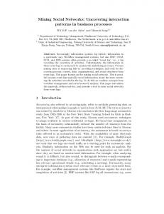
Classification Figure 2: Pipeline

Note that computing sj=1 α(xj , l) · Rj takes time O(m), ˜ where m ˜ denotes the Ps 2 number of non-zero entries in P . Computing the product of D 1 and j=1 α(xj , l) · Rj takes time O(m) ˜ so that the right hand side of equation (10) can be computed in time O(m). ˜ We now have a symmetric diagonally dominant system of linear equations which by Proposition 2 can be solved in time O(m ˜ · log n). Therefore, the time taken to compute the affinity to a fixed community is O(m ˜ · log n) = O(m log n), which is what was claimed. Since we assume our networks to be sparse, m = O(n), and the time taken is O(n · log n) per community. P

4

Experimental Setup

Our experimental setup consists of five parts (see Figure 2) but the respective parts differ slightly depending on whether we test non-overlapping or overlapping communities. We use the LFR benchmark graph generator developed by Lancichinetti, Fortunato, and Radicchi [15, 13], which outputs graphs where the community information of each node is known. From each community in the graph thus generated, we pick a fixed number of 2

This is almost the same as the number m of edges in G, but not quite, since while constructing P from the graph G, we add self-loops on seed nodes and delete edges between adjacent seed nodes, if any. However what is true is that m ˜ ≤ m + s ≤ m + n.

12

seed nodes per community and give these as input to our algorithm. Once the algorithm outputs the affinities of all non-seed nodes, we classify them into communities and finally compare the output with the ground truth using normalized mutual information (NMI) as a metric [4]. We implemented our algorithm in C++ and Python and the code is available online.3 LFR. The LFR benchmark was designed by Lancichinetti, Fortunato and Radicci [15] generates random graphs with community structure. The intention was to establish a standard benchmark suite for community detection algorithms. Using this benchmark they did a comparative analysis of several well-known algorithms for community detection [13]. To the best of our knowledge, this study seems to be the first where standardized tests were carried out on such a range of community detection algorithms. Subsequently, there has been another comprehensive study on overlapping community detection algorithms [26] which also uses (among others) the LFR benchmark. As such, we chose this benchmark for our experiments and set the parameters in the same fashion as in [13]. We briefly describe the major parameters that the user has to supply for generating benchmark graphs in the LFR suite. The node degrees and the community sizes are distributed according to power law, with different exponents. An important parameter is the mixing parameter µ which is the fraction of neighbors of a node that do not belong to any community that the node belongs to, averaged over all nodes. The other parameters include maximum node degree, average node degree, minimum and maximum community sizes. For generating networks with overlapping communities, one can specify what fraction of nodes are present in multiple communities. In what follows, we describe tests for non-overlapping and overlapping communities separately, since there are several small differences in out setup for these two cases.

4.1

Non-overlapping communities

The networks we test have either 1000 nodes or 5000 nodes. The average node degree was set at 20 and the maximum node degree set at 50. The parameter controlling the distribution of node degrees was set at 2 and that for the community size distribution was set at 1. Moreover, we distinguished between big and small communities: small communities have 10–50 nodes and large communities have 20–100 nodes. For each of the four combinations of network and community size, we generated graphs with the above parameters and with varying mixing parameters. For each of these graphs, we tested the community information output by our algorithm and compared it against the 3

At https://github.com/somnath1077/CommunityDetection

13

ground truth using the normalized mutual information as a metric. The plots in the next section show how the performance varies as the mixing parameter was changed. Each data point in these plots is the average over 100 iterations using the same parameters. Seed node generation. To use our algorithm, we expect that users pick seed nodes from every community that they wish to identify in the network. We simulate this by picking a fixed fraction of nodes from each community as seed nodes. One of our assumptions is that the user knows the more important members of each community. To replicate this phenomenon in our experiments, we picked a node as seed node with a probability that is proportional to its degree. That is, nodes with a higher degree were picked in preference to those with a lower degree. For those nodes which were picked as seed nodes, we set the affinity to a community to be 1 if and only if the node belongs to that community and 0 otherwise. Classification into communities. The input to the algorithm consists of the network, the set of seed nodes together with their affinities. Once the algorithm calculates the affinities of all non-seed nodes, we classify them into their respective communities. This is quite easy for non-overlapping communities where we simply assign each node to the community to which it has the highest affinity, breaking ties arbitrarily. Iteration. We extended the algorithm to iteratively improve the goodness of the detected communities. The idea is that after running the algorithm once, there are certain nodes which can be classified into their communities with a high degree of certitude. We add these nodes to the seed node set of the respective community and iterate the procedure. To be precise, in the jþ round, let CAj be the set of nodes that were classified as community A and SAj be the seed nodes of community A. We create SAj+1 as follows: For a fixed ε > 0, choose ε · |CAj | nodes of CAj that have the highest affinity to community A, and add them to SAj to obtain SAj+1 . The factor ε declares by how much the set of seed nodes is allowed to grow in each iteration. Choosing ε = 0.1 gives good results. Repeating this procedure several times significantly improves the quality of the communities detected as measured by the NMI. Each iteration takes O(k · m · log n) time and hence the cost of running the iterative algorithm is the number of iterations times the cost of running it once.

4.2

Overlapping Communities.

The LFR benchmark suite can generate networks with an overlapping community structure. In addition to the parameters mentioned for the non-overlapping case, there is an additional parameter that controls what fraction of nodes of the network are in 14

multiple communities. As in the non-overlapping case, we generated graphs with 1000 and 5000 nodes with the average node degree set at 20 and maximum node degree set at 50. We generated graphs with two types of community sizes: small communities with 10–50 nodes and large communities with 20–100 nodes. Moreover, as in [13], we chose two values for the mixing factor: 0.1 and 0.3 and we plot the quality of the community structure output by the algorithm (measured by the NMI) against the fraction of overlapping nodes in the network. Seed Generation. As in the case for non-overlapping communities, we experimented with a non-iterative and an iterative version of our approach. For the non-iterative version, the percentage of seed nodes that we picked were 5, 10, 15 and 20% per community, with the probability of picking a node being proportional to its degree. For the iterative version, we used 2, 4, 6, 8 and 10% seed nodes per community. Classification into communities. For the overlapping case, we cannot use the naive strategy of classifying a node to a community to which it has maximum affinity, since we do not even know the number of communities a node belongs to. We need a way to infer this information from a node’s affinity vector. For each node, we expect the algorithm to assign high affinities to the communities it belongs to and lower affinities to the communities it does not belong to. We tried assigning a node to all communities to which it has an affinity that exceeds a certain threshold. This, however, did not give good results. The following strategy worked better. Sort the affinities of a node in descending order and let this sequence be a1 , . . . , ak . Calculate the differences ∆1 , . . . , ∆k−1 with ∆j−1 := aj−1 − aj ; let ∆max denote the maximum difference and let i be the smallest index for which ∆i = ∆max . We then associate the node with the communities to which it has the affinities a1 , . . . , ai . The intuition is that, while the node can have a varying affinity to the communities it belongs to, there is likely to be a sharp decrease in affinities for the communities that the node does not belong to. This is what is captured by computing the difference in affinities and then finding out where the first big drop in affinities occurs. Iteration. For overlapping communities, we need to extend our strategy for iteratively improving the quality of the communities found. As in the non-overlapping case, after j rounds, we increase the size of the seed node set of community A by a factor ε by adding those nodes which were classified to be in community A and have the highest affinity to this community. Let v be a such a node. The classification strategy explained above might have classified v to be in multiple communities, say, A1 , . . . , Al . In this

15

case, we assign v to be a seed node for communities A, A1 , . . . , Al . The running time is the number of iterations times the cost of running the algorithm once.

4.3

Normalized Mutual Information

This is an information-theoretic measure that allows us the compare the “distance” between two partitions of a finite set. Let V be a finite set with n elements and let A and B be two partitions of V . The probability that an element chosen uniformly at random belongs to a partite set A ∈ A is nA /n, where nA is the number of elements in A. The Shannon entropy of the partition A is defined as: H(A) = −

nA nA log2 . n A∈A n X

(11)

The mutual information of two random variables is a measure of their mutual dependence. For random variables X and Y with probability mass functions p(x) and p(y), respectively, and with a joint probability mass function p(x, y), the mutual information I(X, Y ) is defined as: I(X, Y ) =

X

X

x∈Ω(X) y∈Ω(Y )

p(x, y) log

p(x, y) , p(x)p(y)

(12)

where Ω(X) is the event space of the random variable X. The mutual information of two partitions A and B of the node set of a graph is calculated by using the so-called “confusion matrix” N whose rows correspond to “real” communities and whose columns correspond to “found” communities. The entry N (A, B) is the number of nodes of community A in partition A that are classified into community B in partition B. The mutual information is defined as: I(A, B) =

nA,B /n nA,B log . (nA /n) · (nB /n) A∈A B∈B n X X

(13)

Danon et al.[4] suggested to use a normalized variant of this measure. The normalized mutual information IN (A, B) between partitions A and B is defined as: IN (A, B) =

2I(A, B) . H(A) + H(B)

(14)

The normalized mutual information takes the value 1 when both partitions are identical. If both partitions are independent of each other, then IN (A, B) = 0.

16

The classical notion of normalized mutual information measures the distance between two partitions and hence cannot be used for overlapping community detection. Lancichinetti, Fortunato, and Kertész [14] proposed a definition of the measure for evaluating the similarity of covers, where a cover of the node set of a graph is a collection of node subsets such that every node of the graph is in at least one set. Their definition of normalized mutual information is: NMILFK

1 := 1 − 2

!

H(A|B) H(B|A) + . H(A) H(B)

(15)

This definition is not exactly an extension of normalized mutual information in that the values obtained by evaluating it on two partitions is different from what is given by normalized mutual information evaluated on the same pair of partitions. However in this paper we use this definition of NMI to evaluate the quality of the overlapping communities discovered by our algorithm. We note that McDaid et al. [16] have extended the definition of normalized mutual information to covers and that for partitions, their definition corresponds to the usual definition of NMI.

5

Experimental Results

As in the last section, we first discuss our results for the non-overlapping case followed by the ones for the overlapping case.

5.1

Non-overlapping communities

Figures 3, 4, and 5 show the plots that we obtained for non-overlapping communities. Figure 3 shows tests for the non-iterative method of our algorithm with 5, 10, 15, and 20% seed nodes per community. The first observation here is that anything less than 10% seed nodes per community do not give good results. With a seed node percentage of 10% or more and a mixing factor of at most 0.4 we achieve an NMI above 0.9 and can compete with Infomap, which was deemed to be one the best performing algorithms on the LFR benchmark [13]. Above a mixing factor of 0.4, our algorithm has a worse performance than Infomap which, curiously enough, achieves an NMI of around 1 till a mixing factor of around 0.6 after which its performance drops steeply. The drop in the performance of our algorithm begins earlier but is not as steep. See Figure 6 for the performance of Infomap and other algorithms that were studied in [13]. Figure 4 shows the results for the iterative approach of our algorithm in the nonoverlapping case. When compared with the non-iterative approach, one can see that 17

even after ten iterations there is a significant improvement in performance (See Figure 5). As can be seen, typically with 6% seed nodes per community we obtain acceptable performance (an NMI value of over 0.9 with the mixing factor of up to 0.5).

5.2

Overlapping communities

Figures 7 and 8 show our results for the overlapping case. In the study of Lancichinetti and Fortunato [13], only one algorithm (Cfinder [19]) for overlapping communities was benchmarked (see Figure 12). The main difference with the non-overlapping case is that typically our algorithm needs a larger seed node percentage per community. This is not surprising since in the overlapping case, we would need seed nodes from the various overlaps as well as from the non-overlapping portions of communities to make a good-enough calculation of the affinities. For graphs of both 1000 and 5000 nodes, our algorithm performs better than Cfinder up to an overlapping fraction of 0.4. We stress that Cfinder has an exponential worst-case running time and would be infeasible on larger graphs. Figures 9 and 10 show the plots for the iterative method (with 10 iterations). A comparison of the non-iterative and iterative method is shown in Figure 11. Iteration yields an improvement in performance, as measured by the NMI, but it is not as dramatic as in the non-overlapping case with the NMI increase being at most 10% at best. The percentage of seed nodes per community required in the iterative approach with a mixing factor of 0.3 is around 8%.

6

Concluding Remarks

Our algorithm seems to work very well with around 6% seed nodes for the non-overlapping case and around 8% seed nodes for the overlapping case. For the non-overlapping case, we can work with a mixing factor of up to 0.5, whereas in the overlapping case a mixing factor of 0.3 and with the overlapping fraction of around 20%. This of course suggests that our algorithm has a higher tolerance while detecting non-overlapping communities and needs either a “well-structured” network or a high seed node percentage for overlapping communities. None of this is really surprising. What is surprising is that such a simple algorithm manages to do so well at all. An obvious question is whether it is possible to avoid the semi-supervised step completely, that is, avoid having the user to specify seed nodes for every community. One possibility is to initially use a clustering algorithm to obtain a first approximation of the communities in the network. The next step would be to pick seed nodes from among the communities thus found (without user intervention) and use our algorithm

18

1000 nodes, small communities, non-iterative

0.8

0.8

0.6

0.6

0.4

0.00.0


1.0

0.4

5% seeds 10% seeds 15% seeds 20% seeds

0.1

0.2

0.3 0.4 0.5 Mixing Parameter

0.2

0.6

0.7

0.00.0

0.8

5000 nodes, small communities, non-iterative

0.8

0.2


0.6

0.7

0.8

0.7

0.8

0.7

0.8

0.7

0.8

5000 nodes, big communities, non-iterative

0.6

0.4

0.00.0

0.1

0.8

0.6

0.2


1.0 Normalized Mutual Information

0.2

1000 nodes, big communities, non-iterative



1.0

0.4


0.1

0.2


0.2

0.6

0.7

0.00.0

0.8


0.1

0.2


0.6

Figure 3: Non-iterative method for non-overlapping communities. 1000 nodes, small communities, iteration 10

0.8

0.8

0.6

0.2

0.00.0


1.0

0.6

2% seeds 4% seeds 6% seeds 8% seeds 10% seeds

0.1

0.2


0.4 0.2

0.6

0.7

0.00.0

0.8

5000 nodes, small communities, iteration 10

0.8

0.2

0.00.0

0.1

0.2


0.6

5000 nodes, big communities, iteration 10

0.8

0.6

0.4



0.4

1000 nodes, big communities, iteration 10



1.0

0.6


0.1

0.2


0.4 0.2

0.6

0.7

0.00.0

0.8


0.1

0.2


0.6

Figure 4: Iterative method for non-overlapping communities.

19

in the 100% o N=1000, S The same trend by Infomod, whereWe theconclu perfo N=1000, B 0.6 is shown N=5000, S with the increase of the ne mance worsens considerably 0.4 0.4 0.4 0.4 method by B N=5000, B work size. Infomap and RN have the best rithms performance 0.2 Blondel et al. 0.2 MCL on th 0.2 Infomod 0.2 Infomap with the same pattern with respect to the size of the ne mark. Since 0 0 0 0.2 0.4 0.6 0.8 0.2 0.4 0.60 0.8 0.2 0.4 work 0.6 and 0.8 of the communities: 0.2 0.4 0.6 up0.8to values of µ ∼ 1/ are alsot very 1 1 Mixing parameter µt to derive the planted both methods are capable partitio we wonder ho 0.8 0.8 1 1 cases. in the1 100% of N=1000, S 1 to the size of than the n to the size graphs to 1 1 N=1000, B 0.6 0.6 N=1000, 0.8 0.8 conclude We that Infomap, theSmance, RN method and th 0.8 0.8 but it gets carried out an mance, but N=5000, S 0.8 N=1000, B 0.8 0.4 0.4 method Blondel et al. are the Sbest algo N=5000, B 0.6 0.6 0.6 by 0.6 The performing same istrs the LFR N=5000, Thetrend sameben 0.6 0.6 LFR N=5000, B rithms on the undirected and unweighted bench 1000 nodes, big communities,0.2 2% seeds 5000 nodes, big communities, 6% seeds 0.2 Infomod Infomap mance worsens cons and 100000 n 0.4 0.4 mance worse 0.4 0.4 1.0 1.0 Clauset et al. workby 0.4 mark. Since0.4Infomap and the method Blondel etcan a 0 0 size. Infomap tests that work size. In al. 0.2 0.2 MCL et al. 0.2 MCL 0.2 0.4 0.6 0.8 0.20.2 0.4Blondel 0.6 etBlondel 0.8 0.8 in the network siz 0.2fast, essentially linearwith Cfinder 0.8 are also very detection one the same with thepatte sam Mixing parameter0µt 0.2 0 0 0 we wonder how good their performance is on much large 0.2 0 0.40.2 0.60.4 0.80.6 0.80.2 0 0.40.2 0.60.4 0.80.6 0.8work and performance of and the com of 0.6 0.6 0.2 0.4 0.6 1 than 0.8 those 0.2 0.4 0.6 0.8 2. For work 1 1 1 graphs considered in7 Fig. this reason w In Fig. 3 we 1 1 both methods are ca 1 1 both method N=1000, S 0.8 0.8 carried out another set of tests of these two algorithms 0.8 0.8 0.4 0.4 Due toof100% the lao N=1000, B in the 100% case in the 0.8 0.8 N=1000, S N=1000, S 0.8 0.8 1 the LFR benchmark, by considering graphs with 5000 N=5000, S N=1000, 0.6 0.6 B 0.6 range comm of theB network. The DM has aBN=1000, fair perforWe conclude tha We ofconclu 0.6 0.6 to the size0.6 0.2 0.2 0.6 0.6 N=5000, N=5000, S We N=5000, S done so also because in th and 100000 nodes. have 0.8 iteration 1 iteration 1network way, the heter mance, but it gets worse if the size increases. 0.4 0.4 0.4 0.4 methodmethod by Blondel by B N=5000, BN=5000, B Clauset 0.4 0.4 iteration 10 iteration 10 can 0.4 et al. 0.4 that be found in the literature on communit 0.00.0 0.1 0.2 0.3 0.4 0.5 0.6 0.7The 0.00.0tests The maximum 0.6 same trend is shown by0.10.2 Infomod, Radicchi 0.8 0.2 Infomap 0.3 0.2 0.4 where 0.5 0.6 the 0.7 perfor0.8 rithms on the LFR rithms on th 0.2 0.2 Infomod Infomod Infomap Mixing Parameter 0.2 Mixing Parameter 0.2 Cfinder 0.2 et al. 0.2 detection one typically usesnetvery small graphs, and th Sim. ann. performa mance worsens considerably with the increase of the 0.4 mark. the Since Infoma mark. Since 0 0 0 0 0 0 work size. performance change considerably onthan largeongraph 0 0.40.2 0.6 0can 0.8 0.2 best 0.40.2 0.60.4 0.4 0.8 0.4 0.8 0.6 0.8 0.8are also the and have the performances, 0.2 0.4 0.6 between 0.8 0.2iterative 0.4 0.2Infomap 0.6 very fast, 0.2 0.4RN0.6 0.6 0.8 0.6 are also verye 0.2 5: MCL Blondel et al. Figure Comparison the and0.8 non-iterative method for0.2 non-overlapping Mixing parameter µ In Fig. 3 we show the performance of the two method Mixing parameter µ 1 1 with the same pattern with Mixing Infomap is st respect to the size of the netparameter µ t t we wonder how good we wonder h 0 communities. t Due toup thetolarge network we decided to pick a broa 0.2 0.4 0.6 0.8 0.8 0.2 0.4 0.6 0.8 0.8 work and of the communities: values of µt size, ∼ 1/2 graphs than those co graphs than 1 1 1 1 range1of community sizes, from 20 Sto 1000 nodes. In th N=1000, S N=1000, partition 0.6 0.6 both methods1 are capable to derive the1 planted carried carried out another out a N=1000, BN=1000, B 0.8 0.8 0.8 0.8 0.8 way, the heterogeneity of the community sizes is manifes 1 0.8 of cases. N=1000, S 0.4 0.4 in the 100%0.8 N=5000, S N=5000, Sthe LFR thebenchmar LFR ben The0.6 maximum degreeN=5000, here to 200. Remarkabl 0.6 conclude 0.6 0.6 N=1000, B 0.6 Radicchi BN=5000, Band 0.6 that Infomap, 0.6 method We the RN andwas thefixed 100000 nodes. and 100000 0.2 et al. N=5000, S 0.2 Sim. ann. 0.8 is wors performance of the method byal.Blondel et al. Clauset etClauset al. 0.4 0.4 0.4 method by0.4 Blondel et al.the are0.4 the best algo-et 0.4 0.4 performing N=5000, B tests that tests that can be ca foo 0 0 than on the smaller graphs of Fig. 2, whereas that 0.2 0.4 0.6 0.8 0.20.2 0.4on 0.6 0.8 rithms the LFR unweighted bench0.2 0.2 and0.2 0.2 Infomap Cfinder Infomod 0.6 typic detection on detection one 0.2 Cfinder 0.2 GN undirected DM Infomap is stable and does not seem to be affected. Mixing parameter µ mark. 0 0 tSince00Infomap and the 0method00 by Blondel et al. performance performance can ch 0.80.8 0.6 0.2 0.4 0.6 0.8 0.2 0.4 0.6 0.8 0.40.20.2 0.60.40.40.80.60.6 0.2in 0the 0.40.2 0.20.60.4 0.40.8 0.6 0.8 0.8 0.4show are also 0.2 very1 0fast, essentially linear network size, In Fig. 3 wet In Fig. 3 we 11 1 1 1 1 11 Mixing parameter µt Infomap et al.larger to the size oftothe ne we wonder how good their performance Blondel is on much Due the la N Due to the 0.2 large net 0.8 0.8 0.8 0.81 1 mance, 0.8 0.8 0.8 0.8 but it gets Nw graphs than those considered in Fig. 2. For this reason we N=1000, S range of com 1 range of community N=1000, S 0.6 0.6 0.6 0.6 N=1000, B 0.6 0.6 0.6 0.6 The same trend is sh carried out another set of tests0.8 of these two algorithms on the 0.8 way, theway, heterogene N=1000, B 0 hete N=5000, S 0.8 0 consi 0.2 0.4 0.4 mance worsens 0.4 0.4 0.4 0.4 the0.4 LFR benchmark, by considering graphs with 50000 N=5000, S 0.4 N=5000, B The maximu The maximum degr Radicchi Radicchi 0.6 N=5000, B work size. Infomap a 0.2 0.2 0.6 MCL 0.6 the performance and0.2100000 nodes. done so0.2 also because 0.2 GN 0.2 DM et EM al. We have 0.2 ann. in the RN Sim. ann.Sim. etBlondel al.0.2 the performa of Clauset et al. 0.4 with the same patter on community 00 be found in the00 literature 0 0 0 tests0 that can the than onthan the on smalle 0.80.2 00.40.2 0.2 0.40.8 0.2 0.40.8 0.6 0.8 0.2 0.4 0.6 0.8 0 0.2 0.40.2 0.6 0.80.6 0.60.4 0.80.60.40.8 0.2 00.4 0.40.2 0.60.4 0.80.6 0.6 0.4 0.8 work and of 3: the Test com 0.20 FIG. Cfinder detection one typically uses very small graphs, and the Infomap is an s 1 1 1 1 Infomap is stable Mixing parameter Mixing µ Mixing parameter µ fomap on both methods arelarg ca 0 performance can change considerably ont large tgraphs. N=50000 Plots0.4 for Infomap, CFinder, the algorithm of Clauset Girvan-Newman (GN), 0.2 0.4 0.6 Figure 0.8 0.8 6: 0.2 0.6 0.8 0.8 0.2et al., N=100000 0.2 0.8 0.8 unweighted lin in the 100% of cases S N=1000, S In N=1000, Fig. the performance of methods. 1 1the two 1 3 Bwe1show Blond Blondel model approach by Ronhovde and on the LFR N=1000, 0.6 et al., and the Pott’s0.6 N=1000,(RN) B 0.6 0.61 Nussinov We conclude that Due to FIG. the large network we toSLFR pickbenchmark a broad0 with 0 decided N=5000, S 0.8 1 0.8 0.8 2: As Tests of thesize, algorithms on the N=5000, 0.8 1 0.8 0.8 benchmark for non-overlapping usual, the NMI-value 1 0 method 0 0.2 0.4(y-axis) 0.6 0.8is plotted 0.2 0.4 0.6 0.4 0.4 communities. 0.4 0.4 by Blondel e N=5000, B N=5000, B range of community sizes, from 20 to 1000 nodes. In this undirected and unweighted links.0.6 Mixing 0.6 0.6performed 0.6 were 0.6 against Tests with 1000 and 5000parameter nodes µt on the 0.2 the 0.2 RN EMmixing factor (x-axis). 0.2 0.2 0.8 LFR way, theInfomod heterogeneity ofon thegraphs community Infomapsizes is manifest. rithms 0.8 0.4 0.4 0.4maximum 0.4 with0.4 big Reproduced B. 0 (B) and small (S) communities. 0 The degreefrom here [13]. was 0fixed to 200. Remarkably, mark. Since Infomap Radicchi 0 0.2 0.4 0.6 0.8 0 0.2 0 0.40.20.20.60.4 0.80.6 0.8 0.2 0.4 0.8 0.2 FIG. 3: Tests ofDM the0.6 algorithm by are Blondel al. and es In 0.6fast, 0.2 GN Sim. ann. also very et al. 0.6 et 0.2 0.2 GN DM the performance of the method by Blondel et al. is worse of the real one, which is more likely found by simulated Mixing parameter µt Mixing parameter µ fomap on large LFR benchmark graphs with undirected an t 0 how good 0 whereas than0 onannealing. the00smaller of0 Fig. 2, that of we Thegraphs Cfinder, the links. MCL the method bywonderDirectedne 0.2 0.4 0.6 0.8 0.2 0.4 0.6 0.8 0 0.4and 0.2 0.6 0.4 0.8 0 0.2 0.40.2 0.60.4unweighted 0.80.6 0 0.80.2 0.80.6 graphs 0.4than 0.4 to obtain a refinement of the community structure. those con Infomap is stable and does not seem to be affected. 1 1 Radicchi et al. do not have impressive performances eiworks. Ignor 1 11 Mixing parameter µt N=1000, S carried out another s A possible extension of our algorithm would be to allow the user to interactively N=50000 to do, may re ther, and display a similar pattern, i.e. the performance FIG. 2: Tests of the algorithms on the LFR with N=1000, B 0.8 0.8 0.2 0.8 benchmark 0.8 0.8 0.2 N=100000 N=1000, SS N=1000, S the LFR benchmark N=5000, 1 Infomap Blondel et al. undirected and unweighted links. is severely affected by the size of the communities (for can extract f specify the seed nodes. The user 0.6 initially0.6supplies a set 0.6 of seed0.6 nodes and allows the N=1000, BN=1000, 0.6 N=5000, B B and 100000 nodes. W 1 1 0 0.8 neglecting lin larger communities it gets worse, whereas for small comN=5000, S 0 N=5000, S output algorithm to find communities. The then checks the0.4 quality of the and, if 0.2 Clauset et al. 0.4 user0.4 0 can 0.2 0 0.4fou B insensitive B. 0.4 and unweighted graphs tests that N=5000, BN=5000, munities it is decent), 0.4 whereas itDirected looks rather ties maybelead 0.6 dissatisfied with the results, can prompt the algorithm to correctly classify some more 0.2 0.2 0.2 0.2 0.8 0.8 Cfinder EM RN 0.2 EM 0.2 RN detection one typica of the one, which is more likely found by simulated 0.4real nodes that The it had incorrectly classified in method the round. end offeatures each 0 current 0 isatanthe 00 the 00In effect, performance can annealing. Cfinder, the MCL and0.6 by Directedness essential real cha ne 0.20.6 0.6 0.40.8 0.80.6 0.6 0.60.60.4 0.80.80.6 0.8 of many 0 0.2 0.2 00.4 00.8 0.20.2 00.40.40.2 0.2 DM GN FIG. 3: ofTes FIG. 3: Tests th round, user additional set of0.4seed nodes until the communities found In Fig. 3 we show th 1performances 1 Radicchithe et al. dosupplies not have an impressive eiworks. Ignoring direction, as one often does or is force parameter µt MixingMixing parameter µt fomap on larg 0 fomap on large LFR Due to the large netw to do, may reduce considerably the information that on ther, and display a similar pattern, i.e. the performance 0 0.2 0.4 0.6 out 0.8 by0 the0.2 0.4 0.6are 0.8 algorithm accurate 0.8 enough for the user. Such 0.8 0.4 0.4 a tool might be useful for unweighted unweighted links. li 1 range of In community is severely affected by the size of the0.6 communities (for can0.6 extract from the network structure. particula visualization. N=50000 way, the heterogeneit 0.8 0.2FIG. 0.2the LFR larger it gets worse, whereas small comlink directedness looking for commun 2:N=100000 of the algorithms on the with FIG.0.4 2: Tests of Tests the algorithms on benchmark S 0.4 Wecommunities wishN=1000, to point out that while thefor running time ofneglecting our algorithm isLFR O(kbenchmark · mwith ·when log n), The maximum degreI Radicchi munities it is decent), whereas it looks rather insensitive ties may lead to partial, or even misleading, results. undirected and unweighted links. N=1000, B 0.6 undirected and unweighted links. 0.2 0 et al. 0.2 0 Sim. ann. N=5000, S the performance of th 0 0.2 0.4 0.6 0.8 1 0 0.2 0.4 0.6 0.8 1 0.4 N=5000, B 0 0 B. Mixing parameter µ than on the smaller B. Direct 0.2 200.4 0.6 0.8 0.2 0.4 0.6 0.8 t 0.2 RN EM Infomap is stable an of the real one, which islikely morefound likely found by simulated Mixing parameter µ of the real one, which is more by simulated t 0 0 0.2 0.4 0.6 0.8 0 0.2 0.4 0.6 0.8 Thealgorithm Cfinder, theBlondel MCL and byDirectedness Directedne FIG. 3:annealing. Tests the by al. the andmethod Inannealing. The ofCfinder, the MCL and theet method by is an 1 Radicchi et al. do not have 1 Mixing parameter µt Blonde works. Ignor impressive performances eifomap onetlarge LFRnot benchmark graphs with undirected and Radicchi al. do have impressive performances eiworks. Ignoring dir 1 to do, may r 0.8 0.8 ther, and display a similar pattern, i.e. the performance unweighted links. ther, and display a similar pattern, i.e. the performance to do, may reduce c can extract affected by the size communities of the communities (for 0.6 is severely 0.6 is severely affected by the size of the (for can0.8 extract from th Tests of the algorithms on the LFR benchmark with larger communities it gets worse, whereas for small comneglecting li 0.4 0.4 larger communities it gets worse, whereas for small comneglecting link dire ted and unweighted links. ties may lea munities it is decent), whereas it looks rather insensitive

Normalize





NormalizedMutual MutualInformation Information Normalized Normalized Mutual Mutual Information Information Normalized


l Information




0.6

Normalized Mutual Information Normalized Mutual Information Normalized Mutual Information Normalized Mutual Information


0.6

nformation



Normalized Mutual Inform

0.6

1000 nodes, small communities, non-iterative, 0.1 mixing parameter



1.0 0.8

0.8

0.6

0.6

0.4

0.00.0


1.0

0.4

5% seeds 10% seeds 15% seeds 20% seeds 0.1

0.2

0.00.0

0.2 0.3 0.4 0.5 Fraction of overlapping vertices

1000 nodes, big communities, non-iterative, 0.1 mixing parameter


0.2

0.8

0.1



0.6

0.4

0.00.0


0.8

0.6

0.2


0.4


0.2

0.00.0




Figure 7: Non-iterative method for overlapping communities on 1000 nodes. 5000 nodes, small communities, non-iterative, 0.1 mixing parameter



1.0 0.8

0.8

0.6

0.6

0.4

0.00.0


1.0

0.4


0.2

0.00.0




0.2

0.8

0.1



0.6

0.4

0.00.0


0.8

0.6

0.2


0.4


0.2

0.00.0




Figure 8: Non-iterative method for overlapping communities on 5000 nodes.

21

1000 nodes, small communities, iteration 10, 0.1 mixing parameter



1.0 0.8

0.8

0.6

0.2

0.00.0


1.0

0.6

0.4

2% seeds 4% seeds 6% seeds 8% seeds 10% seeds 0.1

0.2

0.00.0




0.4

0.8

0.2

0.00.0



1000 nodes, big communities, iteration 10, 0.3 mixing parameter

0.8

0.6

0.4


0.6

0.4


0.2

0.00.0




Figure 9: Iterative method for overlapping communities on 1000 nodes. 5000 nodes, small communities, iteration 10, 0.1 mixing parameter



1.0 0.8

0.8

0.6

0.2

0.00.0


1.0

0.6

0.4


0.2

0.00.0




0.4

0.8

0.2

0.00.0




0.8

0.6

0.4


0.6

0.4


0.2

0.00.0




Figure 10: Iterative method for overlapping communities on 5000 nodes.

22

Undirected and unweighted graphs with overlapping communities


The fact that communities in real systems often overlap has attracted a lot of attention in the last years, leading to the creation of new algorithms able to deal with this special circumstance, starting from the first work by Palla et al. [8]. Meanwhile, a few methods have been developed [12, 39, 45–50], but none of them has been 1000 except nodes, small seeds, networks thoroughly tested, on communities, a parameter bunch of4%specific 0.1 mixing 1.0 real world. Indeed, there have been no taken from the suitable benchmark graphs with overlapping community 0.8 recently [14, 51]. In particular, the LFR structure, until benchmark has been extended to the case of overlapping communities0.6[14], and we use it here. Of our set of algorithms, only the Cfinder is able to find overlapping 0.4 communities. In principle also the EM method assigns to each node the probability that it belongs to any com0.2 munity, but then iteration one would need a criterion to define 1 iteration 10 which, among such probability values, is significant and 0.0 0.2 0.3 0.4 shall 0.5 be neglected. shall be taken0.0or is0.1 not significant Fraction of overlappingand vertices For this reason we report the results of tests carried out with the Cfinder only.

0.8

0.8

0.6

0.6

0.4

N=5000 smin=10 smax=50

0.4

0.2

0.2

µt = 0.1

0 0

0.1

0.2

0.3

µt = 0.3

0 0

0.4

1

1

0.8

0.8

0.6

0.6

0.4

0.4

0.2

0.1

0.3

0.4

3-clique 4-clique 5-clique 6-clique

0.2

µt = 0.1

0

0.2

N=5000 smin=20 smax=100

µt = 0.3

0 0

0.1

1.0

0.2

0.3

0.4

0

0.1

0.2

0.3

0.4

of Overlapping Nodes 5000Fraction nodes, big communities, 6% seeds, 0.1 mixing parameter

FIG. 7: Tests of the Cfinder on the LFR benchmark with 0.8 undirected and unweighted links and overlapping communities. The variable on the x-axis is the fraction of overlapping nodes. The0.6networks have 5000 nodes, the other parameters are the same used for the graphs of Fig. 6. Normalized Mutual Information

D.

Normalized mutual informatio

tive to the community size than to the other parameters.

0.4

0.2

min max

0.2 µ = 0.3 graphs with D.0.2 Undirected and unweighted µt = 0.1 t 0 0 overlapping communities 0

0.1

0.2

0.3

0.4

0.5

0

1

0.1

0.2

0.3

0.4

0.5

1

Normalized mutual information


general we notice that1 triangles (k = 3) yield the worst iteration iteration 410 and 5-cliques give better results. performance, whereas 0.00.0 0.1 0.2 0.3 0.4 0.5 In the two top diagrams Fraction ofcommunity overlapping verticessizes range between 10 and 50 nodes, whereas in the bottom diagrams the from 20 to 100 nodes. By comparing the 9diFigure 11: Comparison between the iterative range and goes non-iterative method for overlapping agrams in the top with those in the bottom we see that communities. the algorithm performs better when communities are (on communities, whereas in the other extreme of big topoaverage) smaller. The networks used to produce Fig. 6 logical mixture and big communities it fails for any value consist of 1000 nodes, whereas those of Fig. 7 consist of of µw . Modularity optimization1 seems to be more sensi1 1 1 5000 of Fig. 6 with Fig. 7 0.8 nodes. From the comparison tive to0.8 the community size than 0.8 to the other parameters. 0.8 N=1000 N=5000 s =10 s =10 of we0.6see that the algorithm 0.6 performs better on networks 0.6 0.6 s =50 s =50 0.4 0.4 0.4 0.4 larger size. min max

0.2

0.2

µt = 0.1

0 0

0.1

VII.

1

0.2

0.3

0.4

µt = 0.3

0 0

0.1

0.2

0.3

0.4

TESTS ON RANDOM GRAPHS 1 3-clique 4-clique 5-clique 6-clique

3-clique overThe0.8 fact that communities in 0.8 real systems often 0.8 0.8 4-clique 5-clique N=1000 N=5000 lap has0.6attracted a lot of attention in the last years, 6-clique leads =20 s =20 0.6 0.6 0.6 An important test of community detection algorithms, s =100 s =100 ing to 0.4 the creation of new algorithms able to deal with 0.4 0.4 0.4 usually ignored in the literature, consists in applying this special starting from the first work by 0.2 µ =circumstance, 0.2 0.2 µto 0.2 them graphs, by definiµ = 0.3 µ = 0.3 0.1 = 0.1random graphs. In random Palla et0 al. [8]. Meanwhile, a0 few methods have been 0 the linking probabilities 0 tion, of the nodes are0.4indepen0 0.1 0.2 0.3 0.4 0.5 0.1 0.2 0.3 0.4 0.5 0 0.1 0.2 0.3 0.4 0 0.1 0.2 0.3 developed [12, 39,Fraction 45–50], but 0none of them has been dent of each other. Inofthis way oneNodes does not expect that of Overlapping Nodes Fraction Overlapping thoroughly tested, except on a bunch of specific networks there will be inhomogeneity in the density of links on the taken from the real world. Indeed, there have been no graphs, i.one.graphs there should no communities. Things Figure 12: Plots for CFinder on the LFR benchmark withbe1000 and 5000 nodes suitable graphs withonoverlapping community are 7:notTests thatofsimple, though. It LFR is certainly truewith that FIG. 6:benchmark Tests of the Cfinder the LFR benchmark with FIG. the Cfinder on the benchmark with overlapping communities. Reproduced structure, until [14, links 51]. and In particular, the LFR from undirected andrecently unweighted overlapping communion[13]. average is whatlinks happens. On the other hand, undirected and this unweighted and overlapping communibenchmark has been of overlapping ties. The variable onextended the x-axistois the the case fraction of overlapping ties. The variable on theofx-axis is the fraction of display overlapping specific realizations random graphs may pseucommunities and have we use here. the Of other our set of alnodes. The [14], networks 1000itnodes, parameters nodes. The networksi. have 5000 nodes, the other docommunities, e., clusters produced by parameters fluctuations are τ1 = 2, τ2 =the 1, hki = 20 and kmaxto = 50. same for theThis graphs of Fig. gorithms, only Cfinder is able find overlapping inthe the linkused density. is why, we do not know of any commercial solvers are for SDD systems that runfor6.ininstance, O(m ·the logmaxn) communities. In principle also the EM method assigns imum modularity of partitions in random graphs is not ++ Since we useshow the method fromHowever, the C a good Eigen Library, it is totime. each node probability that itresults. belongsThe tofactorization any comsmall [25, 52–54]. method should distinIn Figs. 6the and 7 we theCholesky topological munity, then one criterion to define general we noticesuch that triangles (k networks. = 3) yield worst guishto between pseudocommunities and the meaningful mixingbut parameter µt would is implementation fixedneed and aone varies the fraction unlikely that our would be able handle very large Recall which, among such probability is significant and whereas 4- and give to better modules. This is why we5-cliques still expect find results. no comof overlapping nodes between values, communities. We have run performance, T that in Cholesky factorization, matrix In ofmunities coefficients Agraphs. iscommunity decomposed astwobetween LDL shall taken or not significant shall bethe neglected. the two top diagrams sizes range in random We considered types of, thebe Cfinder forisdifferent types and of k-cliques (k indicates For this reason report the clique), results of tests and of 50random nodes, graphs whereas in3 /3 theooperations bottom diagrams the Erd¨ s-R´enyi [55], which have the number nodes oftriangular the with kD =carried 3,is4,diagonal, 5,out 6. In 10graphs: where L isofwe lower and all which takes´anla making with the Cfinder only. range goes from 20 to 100 nodes. By comparing the diit prohibitively expensive for large networks agrams (see, for instance [8]). inThis is notwea see serious in the top with those the bottom that the algorithm performs better when communities (on disadvantage since we expect that in the near future we would have commercialareSDD average) smaller. The networks used to produce Fig. 6 solvers implementing1 the Speilman-Teng algorithm. It would then be interesting to see consist of 1000 nodes, whereas those of Fig. 7 consist of 1 5000 nodes. From the comparison of Fig. 6 with Fig. 7 0.8 size range of real 0.8 networks our algorithm the can handle. N=1000 s =10 we see that the algorithm performs better on networks of 0.6 0.6 s =50 0.4 0.4 larger size. min max

t


t

min max

t

t

min max

0.2

0.2

µt = 0.1

0 0

0.1

0.2

0.3

0.4

0.5

µt = 0.3

0 0

1

1

0.8

0.8

0.6

0.6

0.4

0.4

0.2

0.2

µt = 0.1

0

0.1

0.2

0.3

0.4

0.5

3-clique 4-clique 5-clique 6-clique

VII. N=1000 smin=20 smax=100

µt = 0.3

0 0

0.1

0.2

0.3

0.4

0.5

0

0.1

0.2

0.3

0.4

0.5

Fraction of Overlapping Nodes

FIG. 6: Tests of the Cfinder on the LFR benchmark with undirected and unweighted links and overlapping communities. The variable on the x-axis is the fraction of overlapping nodes. The networks have 1000 nodes, the other parameters are τ1 = 2, τ2 = 1, hki = 20 and kmax = 50.

TESTS ON RANDOM GRAPHS

An important test of community detection algorithms, usually ignored in the literature, consists in applying them to random graphs. In random graphs, by defini23tion, the linking probabilities of the nodes are independent of each other. In this way one does not expect that there will be inhomogeneity in the density of links on the graphs, i. e. there should be no communities. Things are not that simple, though. It is certainly true that on average this is what happens. On the other hand, specific realizations of random graphs may display pseudocommunities, i. e., clusters produced by fluctuations in the link density. This is why, for instance, the max-

References [1] V. D. Blondel, J.-L. Guillaume, R. Lambiotte, and E. Lefebvre. Fast unfolding of communities in large networks. Journal of Statistical Mechanics: Theory and Experiment, 2008(10), 2008. [2] U. Brandes. A faster algorithm for betweenness centrality. Journal of Mathematical Sociology, 25:163–177, 2001. [3] A. Clauset, M. E. J. Newman, and C. Moore. Finding community structure in very large networks. Physical Review E, 70, 2004. [4] L. Danon, A. Diaz-Guilera, J. Duch, and A. Arenas. Comparing community structure identification. Journal of Statistical Mechanics: Theory and Experiment, 2005(09), 2005. [5] L. Donetti and M. A. M. noz. Detecting network communities: a new systematic and efficient algorithm. Journal of Statistical Mechanics: Theory and Experiment, 2004(10), 2004. [6] M. Elkin, Y. Emek, D. A. Spielman, and S.-H. Teng. Lower-stretch spanning trees. In Proceedings of the 37th Annual ACM Symposium on Theory of Computing, pages 494–503. ACM, 2005. [7] M. Girvan and M. E. J. Newman. Community structure in social and biological networks. Proceedings of the National Academy of Sciences, 99(12):7821–7826, 2002. [8] G. H. Golub and C. F. Van Loan. Matrix Computations. John Hopkins University Press, 4th edition, 2013. [9] C. M. Grinstead and J. L. Snell. Introduction to Probability. American Mathematical Society, 1998. [10] R. A. Horn and C. R. Johnson. Matrix Analysis. Cambridge University Press, 2nd edition, 2013. [11] I. Koutis, G. L. Miller, and R. Peng. Approaching optimality for solving SDD linear systems. In Proceedings of the 51st Annual Symposium on Foundations of Computer Science, pages 235–244. IEEE Computer Society, 2010.

24

[12] I. Koutis, G. L. Miller, and R. Peng. A nearly O(m log n)-time solver for SDD linear systems. In Proceedings of the 52nd Annual Symposium on Foundations of Computer Science, pages 590–598. IEEE Computer Society, 2011. [13] A. Lancichinetti and S. Fortunato. Community detection algorithms: A comparative analysis. Physical Review E, 80, 2009. [14] A. Lancichinetti, S. Fortunato, and J. Kertész. Detecting the overlapping and hierarchical community structure in complex networks. New Journal of Physics, 11(3), 2009. [15] A. Lancichinetti, S. Fortunato, and F. Radicchi. Benchmark graphs for testing community detection algorithms. Physical Review E, 78, 2008. [16] A. F. McDaid, D. Greene, and N. J. Hurley. Normalized mutual information to evaluate overlapping community finding algorithms. http://arxiv.org/abs/1110. 2515, 2011. [17] M. E. J. Newman and M. Girvan. Finding and evaluating community structure in networks. Physical Review E, 69, 2004. [18] M. E. J. Newman and E. A. Leicht. Mixture models and exploratory analysis in networks. Proceedings of the National Academy of Sciences, 104(23), 2007. [19] G. Palla, I. Derényi, I. Farkas, and T. Vicsek. Uncovering the overlapping community structure of complex networks in nature and society. Nature, 435:814–818, 2005. [20] F. Radicchi, C. Castellano, F. Cecconi, V. Loreto, and D. Parisi. Defining and identifying communities in networks. Proceedings of the National Academy of Sciences, 101(9):2658–2663, 2004. [21] P. Ronhovde and Z. Nussinov. Multiresolution community detection for megascale networks by information-based replica correlations. Physical Review E, 80, 2009. [22] M. Rosvall and C. T. Bergstrom. Maps of random walks on complex networks reveal community structure. Proceedings of the National Academy of Sciences, 105(4):1118–1123, 2008. [23] D. A. Spielman and S.-H. Teng. Nearly-linear time algorithms for graph partitioning, graph sparsification, and solving linear systems. In Proceedings of the 36th Annual ACM Symposium on Theory of Computing, pages 81–90. ACM, 2004.

25

[24] D. A. Spielman and S.-H. Teng. Nearly-linear time algorithms for preconditioning and solving symmetric, diagonally dominant linear systems. Available at: http://arxiv.org/abs/cs/0607105. Submitted to SIMAX, 2008. [25] N. K. Vishnoi. Lx = b. Laplacian Solvers and their Algorithmic Applications. Now Publishers, 2013. [26] J. Xie, S. Kelley, and B. K. Szymanski. Overlapping community detection in networks: The state-of-the-art and comparative study. ACM Computing Surveys, 45(4):43:1–43:35, 2013.

26