Detecting Spatially Varying Gray Component ... - Semantic Scholar

To be published at the Journal of Electronic Imaging, 2005.

Detecting Spatially Varying Gray Component Replacement With Application in Watermarking Printed Images

Ricardo L. de Queiroz (contact author)

Departamento de Engenharia Elétrica Universidade de Brasília CP 4386, Brasília DF 70919-970 Brazil Ph: +55-61-2735977 Fax: +55-61-2746651 [email protected]

Karen Braun Xerox Corporation 800 Phillips Rd. M/S 128-27E. Webster, NY 14580 USA [email protected]

Robert Loce Xerox Corporation 800 Phillips Rd. M/S 128-27E. Webster, NY 14580 USA [email protected]

1


Abstract – We present a method to include watermarks in printed images. With accurate printer calibration, in theory, the same color under different gray component replacement strategies (GCR) should look the same, under specific viewing conditions. We spatially vary the GCR along the image in a manner that is not perceptible, and we employ an estimation method to detect such changes. The choice of GCR for a given pixel (or region) comprises an additional information channel that embeds a watermark or hidden information. The challenge is how to detect which GCR was used and that is the focus of this paper. For that, we estimate the RGB value of each pixel and the CMYK values intended to be put onto the paper by scanning the printed page. With that information, we can estimate which GCR strategy was used in a given region and retrieve the watermark message. Instead of focusing on a particular watermarking scheme, we are only concerned with the practical aspects of producing a spatially varying GCR and of robustly estimating which GCR strategy was used at a region. Promising GCR detection results are shown to illustrate the method’s potential to watermark printed images.

2


Detecting Spatially Varying Gray Component Replacement With Application in Watermarking Printed Images Ricardo de Queiroz, Karen Braun and Robert Loce Abstract – We present a method to include watermarks in printed images. Under specific viewing conditions and accurate printer calibration, the same color printed using different gray component replacement strategies (GCR) will look the same. We spatially vary the GCR along the image in a manner that is not perceptible, and we employ an estimation method to detect such changes. The choice of GCR for a given pixel (or region) comprises an additional information channel that embeds a watermark or hidden information. The challenge is how to detect which GCR was used and that is the focus of this paper. For that, we estimate the RGB values of each pixel and the CMYK values on the paper by scanning the printed page. With that information, we can estimate which GCR strategy was used in a given region and retrieve the watermark message. Instead of focusing on a particular watermarking scheme, we are only concerned with the practical aspects of producing a spatially varying GCR and of robustly estimating which GCR strategy was used in a region. Promising GCR detection results illustrate the potential of the method to watermark printed images.

I. INTRODUCTION For many reasons, it is desirable to enable data hiding within a digital image: image security, authentication, covert communication, rendering instructions, and providing additional useful information. Some existing digital watermarking methods do not survive the printing process. In fact, most known methods are designed for continuous-tone images and are too fragile to be encoded into a printed page and remain retrievable and invisible. Glyphs [1] and other low frequency methods that can R de Queiroz is with Universidade de Brasília, Brazil, [email protected]. K. Braun is with Xerox Corp. Email [email protected] R. Loce is with Xerox Corp. Email [email protected].

3


be used in a print setting often introduce undesirable textures or lower the spatial resolution of the image. If one has full control of the halftone, watermarks can sometimes be embedded into the halftone design itself [2]-[5]. Other methods applicable to printed pages such as image multiplexing [6] and Xerox Glossmarks ® [7] can also be used. In general, automated watermark retrieval is difficult and the watermarks are not always invisible. To address the seemingly conflicting requirements of invisibility and retrievability of the watermark, one must take into account physical properties of the printing process. For example, we know that very likely the printing will occur at a high resolution, i.e. 600 pixels per inch (ppi) and beyond. Also, the printed images will be viewed at a comfortable distance of the page. Hence, the density of pixels per degree of subtended viewing angle is actually very high and the visual sensitivity will be very low to pixel-level details. Another example of an important physical characteristic is the absorption spectra of the colorants. The three fundamental subtractive primaries, cyan (C), magenta (M), and yellow (Y), are typically used as colorants in printing devices [8]-[11]. All hues can be reproduced with these colorants, however, black colorant is usually also employed for reasons such as extending the dark portion of the color gamut, improving the rendering of neutrals, and reproducing colors with less CMY colorant to save money and reduce pile height. Hence, a transformation is needed to convert from the set of fundamental primaries CMY to the larger set CMYK. The inclusion of the neutral colorant K allows us to substitute in some amount of K for an equivalent darkness neutral mixture of CMY. Thus, for a given color, some K may be added and some CMY subtracted to produce the same perceived color. This colorant substitution method is known as Gray Component Replacement (GCR) [9]. Because color is inherently a threedimensional entity, this addition of a fourth colorant K allows for some redundancy. As a limiting case consider that for much of the color gamut, a given color can be created with either a combination of CMY or with K plus two of those colorants, which is known as a 100% GCR strategy. Lesser amounts of gray component may be substituted creating the potential for multiple GCR strategies. By switching in space between multiple GCR strategies, we can produce the same color in a region, while causing a subtle change in the high-resolution dot pattern that produces the color. Our method embeds hidden data in a manner that is designed for the printing process and does not degrade image texture or resolution. It exploits the properties of a properly designed GCR strategy and applies spatially varying GCR. In Sec. II we describe the watermarking scheme. In Sec. III we explain the enabling technique of detecting the GCR employed for a given pixel or region. Section IV describes experiments that validate the method and indicate that the method holds promise for embedding a significant amount of data. Finally, Sec. V contains the conclusions of this work.

4


II. THE PROPOSED SCHEME: DATA HIDING VIA SPATIALLY VARYING GCR We can view the present watermarking problem as the one of embedding hidden information into the printed image. Without loss of generality, assume we have a message composed of N-ary symbols to embed and that we have at our disposal N GCR schemes. The pixels are received in a color space such as RGB, but note that other color spaces are also valid input.. To enable printing, the pixel representation is converted to a CMY space. As in conventional GCR, the minimum value of the CMY colorant set for a pixel is used to determine K via a GCR curve that relates min(C, M, Y) to K. We have N curves to be chosen for each pixel: GCR1, or GCR2, …, up to GCRN. Hence, from the same RGB data, two or more possible CMYK sets can be generated, depending on the chosen GCR scheme. If the printing path has been properly calibrated, printed CMYK for each of the GCR curves should look the same, at least under the illuminant for which the calibration was performed. Note that under perfect circumstances, different GCRs produce images that look nearly identical and that appearance is presumably robust against small change of illuminants. We refer to the method to embed the bits into a printed page as the “encoder” and we refer to the method for retrieving the message out of the printed paper as the “decoder.” The encoder algorithm is depicted in the top half of Fig. 1. It works as follows: •

The input image is composed of pixels in a color space, such as RGB. The pixels are converted to CMY color space.

•

The image is divided into regions, each region composed of a number of pixels.

•

According to the information bits, in each region, we embed one N-ary symbol. This is done by associating each state of the N-ary symbol to one of the N available GCR schemes.

•

Each pixel is converted to CMYK representation via the chosen GCR for the given region.

•

The image is printed.

The decoder algorithm is depicted in the bottom half of Fig. 1 and can be outlined as the following: •

The image is scanned and aligned such that the decoder analysis can identify and operate on the encoded regions of the image. The scanning produces RGB values at pixel locations.

•

The image is divided into the same regions as employed by the encoder.

•

For each region it estimates the GCR by analyzing the scanned RGB data and estimating the CMYK values that occur on the paper. It then recovers the N-ary symbol in that region using the estimate of CMYK.

•

By recovering each symbol, the hidden message is retrieved.

5


This outline of the GCR encoding/decoding method gives rise to several key questions: 1. How can we estimate CMYK values from scanned RGB values? This is the most significant challenge of the proposed watermarking and retrieval method and is the core of this paper. Estimating the CMYK values enables detecting the local GCR curve. This is discussed in Sec. III. 2. How can we vary the GCR and not cause visible artifacts? Calibration is never perfect and there might be visible differences for some colors, under typical illuminants, when we switch from one GCR to another. We try to calibrate the printing path as well as possible and we suggest that the embedding be applied in a spatially diffuse manner. There are two methods for employing spatial diffusion: make the regions diffuse or make the information diffuse. For example one can blur the transitions of the embedding message and apply error diffusion to avoid a sharp transition between two different GCRs that might cause perceptible artifacts. This crucial issue needs to be thoroughly tested. 3. What happens at regions with little or no GCR (C=0 or M=0 or Y=0) or at very dark regions? Dark regions in the image are not useful for embedding information using this technique, since the excessive dot overlap makes it very difficult to detect black pixels. Also, in light regions, we loose the necessary redundancy since no GCR is needed. These regions can be either skipped, or one can just absorb the error into the error correction (EC) mechanisms. 4. What EC mechanism should be employed? Any efficient correction can be used, including block, convolutional, and turbo codes [12],[13]. Error correction is further discussed in Sec. IV. 5. How can we perfectly register the image? Registration is crucial to enable reading embedded data at any moderate resolution. For example, we target data embedding at 100 or 200 dpi (before error correction). If we do not accurately register the image, dots will be observed out of position and bit error rates will be large, which would force us to considerably drop the resolution. This is another topic that needs to be explored in a future study. Undoubtedly there are many issues to be resolved before implementing a working watermarking scheme. The most crucial one, retrieving CMYK from RGB is discussed in the next section. The other issues will be addressed in future studies.

III. GCR DETECTION There are important practical obstacles for estimating the GCR strategy, particularly because one has to retrieve the CMYK values from scanned RGB data. In general, exact retrieval of CMYK from RGB is not feasible because it is an ill-posed problem. As a result, if one wants to estimate the printed CMYK from

6


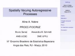
scanned RGB, some information in addition to the color values is required. We exploit the non-overlap property of rotated halftone screens to provide the additional information. Let the printer-side mapping be: RGB-CnMnYnKn , where we have the choice of GCR strategies, hence, of CMYK quadruples to pick for a given RGB triple. On the scanning (decoding) side, a scan of the page would produce some colorimetric R'G'B' values. The estimation problem reduces to estimating the value of n for a particular region. In other words, estimate which GCR was used in that region. If the color correction process used by the printer and its printer characterization are sufficiently accurate, we expect the colorimetric RGB values of the printed page, as produced by a low resolution scanner, to resemble the input RGB values, i.e. RGB=R'G'B'. Therefore if we can estimate the actual CMYK amounts put onto the paper we would have the RGB and CMYK values from which to estimate the GCR strategy. We derive estimates of the actual CMYK data from a high-resolution scan, while the scanner RGB values are found from a low resolution scan. The non-trivial part is to estimate K from the scan. To simplify, we use RGB values scanned at a resolution higher than the print resolution, where we might be able to discern ink dots and estimate K. The process is illustrated in Fig. 2. There are 3 different resolutions involved: the printing, scanning and watermarking resolutions. For example printing might take place at 600 ppi, scanning may be at 1200 ppi and the watermarking may be embedded and detected at a rate of 120 ppi, i.e. transmission rate is 120 bits per inch (bpi). A. Estimating K from a high-resolution scan If we assume halftoning with rotated screens, it is likely that all the four CMYK dots do not overlap completely. Actually, the amount of overlap of CMY dots covers a small area percentage at mid tones. Assume the printed image has perfect dots and that the scanner can resolve the dots and their overlaps. In this hypothetical case, the scanned RGB values only assume a small number of combinations that depend on the geometry of the dots against the scanner resolution. If each of the scanned hi-resolution RGB values for a given pixel is very low, then that pixel possesses a black color. A black-colored pixel is indicative of a K dot. This K assumption is a good approximation because for low values of RGB there must be a K dot or the overlap of CMY dots. Since the overlap area of CMY dots is small due to the rotated screens, it is more likely the black pixel indicates the presence of a K dot. Thus, we estimate the K signal by the following procedure. The scanned RGB values are inverted to obtain CMY estimates, then K is estimated as K=min(C, M, Y)=1−max(R, G, B). Note that, except for when there is full CMY overlap or a K dot, at least one of the RGB values will be near maximum (paper) so that the estimate yields K. Let Kh be an estimate of the K toner image derived from a high resolution

7


scan. We assume that information is embedded in the image at a lower spatial resolution than the scanned image. Let S be a suitable operator to reduce the image from the scanner resolution to the watermark resolution. For example, S can be a sequence of blurring filters followed by sub-sampling. Kh may be written Kh = S(min(C, M, Y)) = S(1−max(R, G, B))

(1)

Even though the formula for Kh resembles a formula for generating K in a 100% GCR strategy, its present use is distinct from that relationship. In fact, its use is limited to high-resolution scanned data where the printer dots can be discerned. We call this method the deterministic approach. A difficulty with the deterministic approach is that the luminance of a black dot depends on the luminance of the patch it is printed on, as well as the size of the dot itself. A small black dot on a light colored area has a higher luminance than a large black dot on a darker background. Thus a more empirical approach is employed, whereby K is estimated by adaptive thresholding. Scanned pixels below a particular luminance level are assumed to be black. The idea is to determine how many pixels in each region correspond to black dots. Thus, we varied the threshold level based on the average luminance of the region. For each average gray value it is desirable to apply a threshold that maximizes the distinction between two GCRs. The threshold-vs-luminance relation was obtained by training on a number of scanned patches. Each patch was printed using both GCR1 or GCR2 strategies, by which we denote as P1n, and P2n, where n is the patch index or counter. For the n-th pair of patches, the average luminance is taken as the average, i.e. Ln = mean((P 1n + P2n)/2). Ideally, the luminance of both patches should be equal. However practical limitations in calibration and printing, along with the fact that the scanner is not the calibrated observer, might make the luminance of the patches slightly different. We apply a threshold to estimate whether the pixel is a K pixel or not. We test each threshold τ (0 k) , Sum(P2n > k) / Sum(P1n > k)}

(2)

Then, every patch has an (Ln, τn) pair. Figure 3 shows a typical relation between thresholds and average luminance values. We approximated this behavior by a piecewise-linear curve τ(L) that passes through

8


the following (L,τ(L)) points: (0 , 0) , (25 , 20) , (100 , 40) , (150 , 80) , (210 , 125) , (255 , 255). (This is a printer dependent curve.) Using this curve, Kh is estimated as: Kh = S( T(t (L), L) )

(3)

where T(t,x) is a threshold function such that T(t,x)=255 if x>t and T(t,x)=0 otherwise. In other words Kh is estimated as: •

Convert the RGB high resolution data into gray L, for example using L = 0.253R + 0.684G + 0.063B.

•

Blur the image using a large filter to get the local average luminance values L'.

•

For each pixel, given L ', look-up the associated threshold τ from the above τ(L) curve. Then, threshold L to obtain K as a binary dot.

•

Reduce the image to any suitable lower resolution. This is the same resolution in which RGB will be analyzed.

B. Maximum likelihood estimation of the GCR Different GCR strategies generate images that may look different except under the illuminant for which the color correction was derived. This is known as illuminant metamerism [8]-[11]. This effect may be exacerbated by metamerism between humans and typical scanners. That is, two colors (made up of two different CMYK combinations) that match for humans may not match for the scanner because its spectral sensitivity is different from the human visual system. Whereas Kh exploited high resolution and halftone overlap geometry to extract an amount of K toner, we can define Kl as a low resolution measure of the darkness of a local area and provides a measure of the capacity of that area to possess K toner. In this case, the Kl values are related to the RGB values in an average colorimetric way and purposely do not comprehend microscopic halftone dot geometry. If we assume there is only a high-resolution scanner, the Kl data can be reduced (using S) so that Kl = 1 − max(S(R ), S(G), S(B))

(4)

Note the important difference between (1) and (4). One can derive the luminance value from the low-resolution scans as L = 0.253 S(R ) + 0.684 S(G) + 0.063 S(B) and we now have two other quantities to normalize the value of Kh against some reference point so that we can estimate the GCR used (hence, the embedded bit data) by analyzing the triplet {Kl , Kh , L } somehow. Then, the GCR detection problem becomes similar to the one in classical

9


estimation theory [14]. The N-ary symbol is transmitted over a noisy channel. Given the reception of some Kh value, one needs to estimate which symbol was actually used. Let P{A|B} denote the conditional probability of an event A given B and E{x|B} denote the conditional expectation of a random variable. It is known that for equiprobable sources, the maximum likelihood estimation is the symbol that maximizes

max P{K h − q i | K l , L} , i

(5)

where qi are the values of Kh one would produce in a noiseless environment, i.e. the values obtained if there was perfect estimation of Kh. In other words, if GCR=n, then η=Kh–qn is the noise input the system. Note that in this simplified model we have not incorporated noise from measuring either Kl and L. For noise densities with a strictly decaying spectrum, one wants to choose the closest qi to the given Kh. Let us define β(n, Kl, L) ≡ E(Kh | Kl, L, GCR=n)

(6)

then, one can show that for a given well-behaved noisy framework, the qi values are well estimated by min {K h − β (i, K l , L)} . i

(7)

Summarizing, the steps for detecting one out of N GCRs are: •

In the training session, find one image or region that was processed with each GCR. For each region or image compute β(n, Kl, L)=E(Kh | Kl, L, GCR=n), i.e. the average value of Kh for each (Kl,L) pair.

•

In the on-line detection phase, select β that is the closest to the received Kh. Note that in the binary case, there are only two values to compute, β(1, Kl , L) and β(2, Kl , L), so

that the algorithm is equivalent to setting up a threshold τ(Kl , L) = [β(1, Kl , L) + β(2, Kl , L)] / 2

(8)

so that Kh is simply compared to a threshold τ(Kl, L). If Kh>τ, then we pick GCR2, else we pick GCR1. It is very simple and the array of thresholds for each Kl and L, typically of size 256x256, can be setup beforehand. Hence, detection can be made with one look-up and one comparison.

10


C. LUT-based estimation of the GCR To train the system, we create an image (preferably of a test target of patches) with the GCR strategies of interest. For every pixel, a quintuple is organized: {R, G, B, K, Q} where Q is a discrete number telling which GCR was actually used to print that given scanned pixel. We are now left with the task of mapping the RGBK hypercube into one number Q. The training algorithm works by simple majority. •

Break the RGBK hypercube into N cells.

•

For every pixel in the image

•

•

o

Find its RGBK cell

o

Fill in its Q value

At the end, for each cell, o

Compute the histogram of Q values

o

Associate the cell with the most “popular” Q value for that cell.

Make a LUT with the RGBK values as input and Q as output

Each cell maps the RGBK value to its most likely GCR strategy. To ensure that no cells are empty, we start by running the above training algorithm with a partition of RGBK into 2x2x2x2 cells. If, at the end of training, any of the cells is still empty, assign a random Q value to it. Then we repeat the process for a 4x4x4x4 cell partition. If at the end of the process we obtain any empty cell, make it inherit the Q value from the corresponding position in the 2x2x2x2-partition stage. For non-empty cells, we use the 4x4x4x4 value. We repeat the process for 8x8x8x8. Any empty cells inherit the corresponding Q value from the 4x4x4x4 partition stage. The process is repeated yet one more time to obtain 16x16x16x16 cells, inheriting Q values from the 8x8x8x8 partition stage. We judged the 16x16x16x16 partition might be accurate enough to map RGBK values to a few GCRs like 2, i.e. a Q=0 or Q=1 decision. The run-time detection algorithm works as follows: •

In the high resolution image, estimate K.

•

Reduce the K image to low resolution.

•

Reduce RGB scanner data to low resolution.

•

For every pixel in the low resolution image o

Compute the RGBK quadruple

o

Feed RGBK into the cell LUT, retrieve Q which is the GCR estimation

11


IV. EVALUATING EMBEDDING POTENTIAL We have not yet implemented a real data embedding system. Future work will deal with registration and with diffuse embedding patterns. We did not switch GCR on a pixel by pixel basis but we set up whole images or large regions with each of the GCRs and measured detection error rates in each region. This gives a very good measure of the method’s embedding potential, apart from any registration errors.

A. Method I - Deterministic estimation of K plus ML estimation of GCR. In an example, we processed several images using two different GCRs. The GCR strategies were devised using color calibration tools tuned for a Xerox DocuColor 2060 printer which uses a 600-ppi rotated linescreen. Printer calibration was a bit off so the variation of GCR caused a very small but sometimes noticeable change in appearance. The images were printed at the DC2060 and scanned using a Scitex scanner at true 2000 ppi. The images were reduced (S) using running averaging filters and straight subsampling, until reaching a factor of 10:1 in each direction, i.e. 200 ppi. This is the watermark resolution. The left side of each image was processed using GCR1 while the right side was processed using GCR2, except for the two images that were used for training. One training image was processed using GCR1 in its entirety, while the other was only processed using GCR2. All images (including the training images) were printed on the same page to simplify the experiment, but this certainly was not necessary. The recovered 200-ppi RGB composite image is shown in Fig. 4. The images that were used for training are indicated. Figure 5 shows the corresponding luminance L, Fig. 6 has the Kl values, and Fig. 7 shows Kh for the same image. The detected image is shown in Fig. 8. Since data cannot be effectively embedded in very light or dark areas because they have mostly uniform ink coverage, we decided to exclude these areas from processing. In regions where L was larger then 240 or less than 15, the pixels in Fig. 6 were marked as gray, i.e. not embedded. The bit error rates (BER) for these example images are shown at Table I.

B. Method II – Empirical estimation of K plus LUT-based estimation of GCR. In this set of tests, we used scans made on a desktop 1200 ppi scanner of prints made on a Xerox Phaser 7700. After reduction of 10:1, the watermark detection (RGBK data) resolution is 120 bpi. Figure 9 depicts a comparison of the amount K used during printing and the amount of K detected from the

12


scanned data. The same image was printed under two different GCRs and each image was subject to our GCR detection method. Figure 10 shows the result of Method I while Fig. 11 shows the result for Method II. The left half of each Figure (10 or 11) was made with GCR1 and the right half with GCR2. White pixels indicate that GCR1 was detected and black pixels that GCR2 was detected. So a perfect result would be an image with the left half white and the right half black. Comparing Figs. 10 and 11, we can see that the second technique is much less noisy for this class of printers. Method I led to too many noisy patches. A comparison of detection efficiency is shown in Table II. We, then, computed the percentage of times there was a correct estimation for each method and GCR. These results do not include the detection errors from the borders between the patches. However, they do include patches where it is impossible to embed information, namely those where one or more of the pre-GCR C, M, or Y values is zero.

C. Channel rate and distortion considerations The image embedding method can be viewed as a communications channel so that we can borrow information theory results for it. The problem is that we have not fully characterized the channel yet. However, based on the results for both methods we have not seen an average BER (1 to 0 and vice-versa) of more than 30%. Please note that these tests were carried for a low-resolution RGBK set at 200 and 120 dpi. The channel is not symmetric, as the results show. It is not stationary either since contiguous regions typically have similar colors. We can homogenize the error by logically scrambling the pixel locations before embedding, and equalizing (biasing) the information so that the channel should appear to the encoder as a binary symmetric channel (BSC). The BSC is well known in the literature and let us assume the error probability Pe to be 1/3 (1/3 of the bits are wrong in average). It is known that the equiprobable BSC capacity for Pe=1/3 is about 0.0817 bits/symbol [13]. At 200 ppi, there are 40000 pels/in2, hence the channel capacity would be 3268 bits/in2. At 100 ppi, assuming the same error rate, the capacity drops to 817 bits/in2 or near 100 bytes/in2. If we construct one of the simplest error correction mechanism there is, the recursive use of block codes, e.g. the (7,4) Hamming code [13], we can protect the channel until any prescribed BER. At each step the embedding rate falls by 4/7, but BER drops by 0.627. The BER vs. bit rate curves for both 100 ppi and 200 ppi watermarking RGBK data, assuming the equiprobable BSC with Pe=1/3 are shown in Fig. 12. Figure 12 is just an example. Other channel coding schemes will greatly improve the curves in Fig. 12. The nature of the GCR strategies that are used will increase or decrease the probability of correct detection, depending on how much they differ. For example, excellent detection would be attainable from

13


using 100% GCR and no GCR. However this would result in more visibility of the embedded signal as a result of metamerism than two GCR strategies that are more similar. The watermark visibility is not computed in any trade-off, so that the best strategy is to make the two GCR strategies not too dissimilar. The inclusion of visibility constraints in the rate-distortion trade-off is left to a future work.

V. FINAL REMARKS In many applications where a watermark is embedded, all the embedded bits are taken together to embed just one bit that is used to answer the question: “is the watermark there or not?”. The rate distortion analysis of the method assuming a BSC with 1/3 error probability indicates that a reasonable amount of bits can be embedded with a reasonable error probability. It is surely sufficient to simply recognize a watermark (the one bit embedding) or to carry small payloads. In other words, the method has large bit rate and large BER, so that good error correction capabilities are essential. Certain colors in an image are not useful for embedding information by varying GCR, namely those that have no K replacement. For example, CMY values of (c,m,0) will be converted to (c,m,0,0) using either GCR technique. Ideally, these would be eliminated from the encoding/decoding process in some way or perhaps information could be redundantly embedded such that information erased in one region of the image could be found in another region. At this point, no such scheme has been devised. We use training images, but the technique would also work if the nature of the GCR algorithms was known and a fully color-characterized system was used. The training images eliminate the need for such careful calibration. The detection might be improved by using the spatial orientation of the dots on the page. Black dots are expected to appear at a 45° angle, which would differentiate them from other dots. Attempts at using this information have not been successful yet. Inspection of the results shows the potential of GCR detection in watermarking. A working system is far from being developed. There is much analysis and fine-tuning that can be done. Future work is planned on (i) improving print path calibrations and extending the family of test printers and technologies; (ii) including error correcting capabilities and analyzing the channel capacity i.e. how much payload can we embed after error recovery; (iii) optimizing embedding patterns; and (iv) reliable registration. In any case, the process has considerable potential and the detection method appears to be robust enough to warrant further research leading to practical applications.

14


REFERENCES [1] D. L. Hecht, “Printed Embedded Data Graphical User Interfaces, IEEE Computer, pp. 47-55, Mar. 2001. [2] K. T. Knox and S. Wang, "Digital watermarks using stochastic screens -- a halftoning watermark," Proceedings of the SPIE International Conference on Storage and Retrieval for Image and Video Databases V, vol. 3022, pp. 310-316, San Jose, CA, US, Feb. 1997. [3] S. Wang, K. T. Knox, Embedding digital watermarks in halftone screens, Proceedings of SPIE Security and Watermarking of Multimedia Contents II, Vol. 3971, pp. , San Jose, CA, US, Jan. 2000. [4] M. S. Fu, O. C. Au, Data hiding in halftone image by pixel toggling, Proceedings of SPIE Security and Watermarking of Multimedia Contents II, Vol. 3971, pp. , San Jose, CA, US, Jan. 2000. [5] Z. Baharav and D. Shaked, “Watermarking of digital halftones,” Electronic Imaging, Vol. 3657, pp. 307-313, Jan. 1999. [6] G. Sharma, R. P. Loce, S. J. Harrington, and Y. Zhang, “Illuminant multiplexed imaging: GCR and special effects,” Proc. IS&T/SID Eleventh Color Imaging Conference: Color Science, Systems and Applications, Scottsdale, AZ, pp 266-271, Nov. 2003. [7] C. Liu, S. Wang, and B. Xu, “Authenticate Your Digital Prints with Glossmark Images,” in Proc. NIP20: The 20th International Congress on Digital Printing Technologies, Salt Lake City, UT, US, Nov. 2004. [8] R. W. G. Hunt, The Reproduction of Color, Fountain Press, Toolworth, England, 2000. [9] R. Bala, “Device characterization,” Chapter 5 in Digital Color Imaging Handbook, G. Sharma Ed., CRC Press, Boca Raton, FL, US, 2003. [10]

G. Sharma, “Digital Color Imaging,” IEEE Trans. On Image Processing, Vol. 6, pp. 901-932,

1997. [11] E. Giorgianni and T. Madden, Digital Color Management, Addison-Wesley, Reading, MA, US, 1997. [12] J. B. Anderson and S. Mohan, Source and Channel Coding, Kluwer Academic Press, Norwell, MA, US, 1991. [13] C. Schlegel and L. Perez, Trellis and Turbo Coding, Wiley-IEEE Press, 2003. [14] J. M. Wozencraft and I. M. Jacobs, Principles of Communications Engineering, Wiley, New York, US, 1965.

15


Dr. Ricardo L. de Queiroz received the Engineer degree from Universidade de Brasilia , Brazil, in 1987, the M.Sc. degree from Universidade Estadual de Campinas, Brazil, in 1990, and the Ph.D. degree from University of Texas at Arlington , in 1994, all in Electrical Engineering. In 1990-1991, he was with the DSP research group at Universidade de Brasilia, as a research associate. He joined Xerox Corp. in 1994, where he was a member of the research staff until 2002. In 2000-2001 he was also an Adjunct Faculty at the Rochester Institute of Technology. He is now with the Electrical Engineering Department at Universidade de Brasilia. Dr. de Queiroz has published extensively in Journals and conferences and contributed chapters to books as well. He also holds 35 issued patents, while many others are are still pending. He received several scholarships and grants from the Brazilian government and universities. He is an associate editor for the IEEE Signal Processing Letters. He has been actively involved with the Rochester chapter of the IEEE Signal Processing Society , where he served as Chair and organized the Western New York Image Processing Workshop since its inception until 2001. He was also part of the organizing committee of ICIP'2002. His research interests include multirate signal processing, image and signal compression, and color imaging. Dr. de Queiroz is a Senior Member of IEEE and a member of IS&T.

Karen Braun received her B.S. degree in physics from Canisius College in 1991 and her Ph.D. in imaging science from Rochester Institute of Technology in 1996. Since then, she has worked in the Xerox Innovation Group at Xerox Corporation, focusing on color reproduction, gamut mapping, and color perception. Karen has published numerous journal articles on color appearance modeling and gamut mapping, presented her work at conferences, and co-authored Recent Progress in Color Science in 1997. Karen has been an active member of ISCC for ten years. She helped create the first student chapter of the ISCC at RIT in March 1993, and served as its first president. She was a Board Member for three years, associate editor of ISCC News, a voting delegate for three years, and chairman of the Individual Member Group (IMG). Karen is an active member of IS&T. She has served on the Technical Committee of the IS&T/SID Color Imaging Conference for the six years, and served as Poster Chair for three years.

16


Robert Loce is a Principal Scientist in the Wilson Center for Research and Technology, Xerox Corporation. He joined Xerox in 1981. While working in optical and imaging technology and research departments at Xerox, he received a BS in Photographic Science (RIT 1985), an MS in Optical Engineering (UR 1987), and a PhD in Imaging Science (RIT 1993). His current work involves development of image processing methods for color electronic printing. He is currently an associate editor for Journal of Electronic Imaging, Real-Time Imaging, and IEEE Transactions on Image Processing. He is a member of SPIE and IEEE.

17


Table I – BER for several images and for both GCRs as references. Watermark resolution is 200 bpi. Image

1

2

3

4

5

GCR-1

0.0300

0.2753

0.1546

0.0867

0.0321

GCR-2

0.3506

0.2384

0.3212

0.1562

0.3191

Table II. BER for both methods using patches images from Figs. 9-11. Watermarking detection resolution is 120 bpi. Method I II

GCR-1 0.28 0.18

18

GCR-2 0.47 0.29


FIGURE CAPTIONS Figure 1. Top half shows inserting the watermark. Bottom half shows extracting the watermark. Figure 2. GCR estimation steps diagram. Figure 3 – Average local luminance value against best threshold. Figure 4 - Scanned image reduced to 200dpi. Figure 5 - Luminance (L) corresponding to Fig. 4. Figure 6 - Value of colorimetric K (Kl) obtained from the image in Fig. 4. Figure 7 - Estimated K value (Kh) from the high resolution (2000 dpi) scan. Image size reduction to 200 dpi occurs after K is estimated. Figure 8 - Detected information. Gray values indicate excluded areas where L was out of bounds 15-240. The original information consists of different GCR for the left and right side of each image. The two training images were fully processed using one GCR, a different GCR each, of course. Figure 9 – Original K values before printing (left) and estimated K values after printing and scanning (right). Figure 10 - Result for patches image using Method I. Left image was printed under GCR-1 while the one on the right was printed under GCR-2. The part on the left should be white and the one on the right should be all black. Figure 11. Result for patches image using Method II. Left image was printed under GCR-1 while the one on the right was printed under GCR-2. The part on the left should be white and the one on the right should be all black. Figure 12 - Representative rate vs. distortion characteristics of the system. The above curves relate the BER and the payload capacity, assuming both 200 bpi and 100 bpi watermarking resolution. We assumed an equiprobable symmetric channel with 1/3 probability of error and channel coding via recursive application of Hamming block codes.

19


Print C1M1Y1K1 RGB

C2M2Y2K2

CMY

CNMNYNKN

Information bits

Scan

Estimate RGB

CMYK

determine GCR

Retrieve n

Figure 1. Top half shows inserting the watermark. Bottom half shows extracting the watermark.

20


Printout RGB Hi-res

K Hi-res

RGB Low-res

K Low-res

Guess GCR from low-res RGBK values

Figure 2. GCR estimation steps diagram.

21


Figure 3 – Average local luminance value against best threshold.

22


Training

Figure 4 - Scanned image reduced to 200dpi.

23


Figure 5 - Luminance (L) corresponding to Fig. 4.

24


Figure 6 - Value of colorimetric K (Kl) obtained from the image in Fig. 4.

25


Figure 7 - Estimated K value (Kh) from the high resolution (2000 dpi) scan. Image size reduction to 200 dpi occurs after K is estimated.

26


Figure 8 - Detected information. Gray values indicate excluded areas where L was out of bounds 15-240. The original information consists of different GCR for the left and right side of each image. The two training images were fully processed using one GCR, a different GCR each, of course.

27


Figure 9 – Original K values before printing (left) and estimated K values after printing and scanning (right).

28


Figure 10. Result for patches image using Method I. Left image was printed under GCR1 while the one on the right was printed under GCR-2. The part on the left should be white and the one on the right should be all black.

29


Figure 11. Result for patches image using Method II. Left image was printed under GCR1 while the one on the right was printed under GCR-2. The part on the left should be white and the one on the right should be all black.

30


10

Bit error rate

10

0

100dpi

-1

10 -2

10

10

200dpi

-3

-4

10 -5 10

-1

10

0

10

1

10

2

10

3

10

4

10

5

Bits per sq. in.

Figure 12 - Representative rate vs. distortion characteristics of the system. The above curves relate the BER and the payload capacity, assuming both 200 bpi and 100 bpi watermarking resolution. We assumed an equiprobable symmetric channel with 1/3 probability of error and channel coding via recursive application of Hamming block codes.

31