Detecting inexplicable behaviour - Semantic Scholar

Detecting inexplicable behaviour Hannah Dee and David Hogg School of Computing University of Leeds Leeds, LS2 9JT, UK [hannah][dch]@comp.leeds.ac.uk Abstract

This paper presents a novel approach to the detection of unusual or interesting events in videos involving certain types of intentional behaviour, such as pedestrian scenes. The approach is not based upon a statistical measure of typicality, but upon building an understanding of the way people navigate towards a goal. The activity of agents moving around within the scene is evaluated based upon whether the behaviour in question is consistent with a simple model of goal-directed behaviour and a model of those goals and obstacles known to be in the scene. The advantages of such an approach are multiple: it handles the presence of movable obstacles (for example, parked cars) with ease; trajectories which have never before been presented to the system can be classified as explicable; and the technique as a whole has a prima facie psychological plausibility. A system based upon these principles is demonstrated in two scenes: a car-park, and in a foyer scenario 1.

1 Introduction When you monitor a pedestrian scene, a number of different behaviour patterns can be observed. People walk along pathways and cars are driven along roads, and occasionally people will take shortcuts or get into a car or stop for a chat. Very occasionally, someone will do something different or interesting – something that does not fit our general understanding of what behaviour goes on in that scene. The aim of this research is to develop a framework for the detection of these interesting events. A number of systems have been constructed which go some way towards addressing this problem. One approach is exemplified in [4], in which the typicality or otherwise of pedestrian trajectories is assessed based upon learned models of absolute location and speed over time. In [6], a model of the paths within a scene is constructed based upon the behaviour of pedestrians, and this path model can subsequently be used to detect unusual trajectories. The relationships between objects can also be used to judge typicality [7]. There are drawbacks to all of these approaches when applied to a changing environment (such as a car park): the first two are too closely tied to the global environment, and the third to the objects within that environment. All three approaches ignore the underlying 1 The foyer scenario is from the PETS2004 dataset, which comes from the EC Funded CAVIAR project/IST 2001 37540

intentional nature of the agents within the scene – indeed, they are thought of as objects, rather than agents. The philosopher Daniel Dennett has written widely on the nature of explanation, and has long been an advocate of what he calls “the Intentional Stance” – see, for example, [3]. When we adopt the intentional stance towards an object, we reason about its past and future behaviour on the grounds of its supposed beliefs and desires. Humans and animals are inherently intentional creatures – we behave in a goal-directed fashion, and the visible component of our behaviour can often be explained with reference to our goals (indeed, it can often only be explained with reference to our goals). Each of the computer vision systems outlined in the previous paragraph adopt what Dennett calls the physical stance in the analysis of human behaviour – they do not take into account the psychology of the agents within the scene and as such miss out on many simplifying assumptions. The work we describe here is the first to incorporate a simple model of psychological function and thus adopt the intentional stance in the prediction and classification of human visible behaviour. Our approach is to build a model of intentional, goal-directed navigation and compare observed behaviour to that. Behaviour patterns defined as interesting are those which do not fit our assumptions, and rather than being interpreted as atypical or abnormal, any interesting events detected by such a method are best described as “inexplicable”.

2 Determining which goals within the scene may be goals of the agent: Goals, Sub-goals, and navigation In those pedestrian domains typically subject to surveillance, people have particularly well-defined goals which are easy to infer from their visible behaviour. For example, in a car park agents either wish to get from an exit to their car, from their car to an exit or from an exit to an exit (for example, when taking a short cut). We therefore define a goal as an exit: a place where an agent can leave the scene. We wish to characterise the behaviour of the agents within our scenes in terms of these possible goals, and so we need a model of how people actually navigate towards a goal. One strategy for planning the route to an exit would be to seek the shortest path. In general, the shortest path is a series of straight line segments through free-space, terminating at tangential points on the obstacles, and connected by curved segments around the boundaries of obstacles. Instead of using the shortest path we make the more general assumption that our agent chooses a piecewise linear path between tangential points (which we call sub-goals). If a goal is accessible by one turn and later by two, this goal has become a less likely explanation for the agent’s actions. These sub-goals are central to our approach. Simply put, sub-goals allow people to go around corners – if there is not a direct path to a particular goal from the current location, that does not mean that goal is not a possible explanation for the behaviour in question: there may exist an interim position with a direct path to the goal and from the current position. Such a position is defined as a sub-goal. Without sub-goals, our thesis could be distilled into the sentence “People generally walk towards goals in straight lines”. With sub-goals, it becomes the more interesting “People generally behave in a goal-directed fashion”.

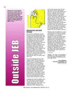
2.1 Initial selection of sub-goal candidates The construction of sub-goals is based upon geographical information about the location of obstacles, the current location of the agent within the scene x and their direction of motion θ , and upon counterfactual reasoning. From the current position x, a segment of the scene is investigated. We are interested in discovering places to which the agent could travel directly and that allow the agent access to places to which they cannot travel directly. These places are points where agents can choose to change direction, and these places are just after obstacles. Initially, we label pixels as either being directly visible from x (labelled V), obstacle (labelled O), or not visible from x (labelled N). Then we look for possible sub-goals in the direction of the agent’s travel, allowing one radian either way for deviation from the straight line path2 . Thus those pixels that are classified as V and which lie within an arc
through x from θ 1 to θ 1 are investigated further, searching for pixel neighbourhoods containing all three labels of pixels. Regions containing all three types of pixel are candidate sub-goals – that is, the agent at x might be headed towards x  (it is directly visible and within their angle of vision), and were they at x  they would be able to see more of the scene (it neighbours upon areas that are not directly visible from x). When a candidate sub-goal has been found, scanning starts from x  in all directions, pixels are labelled and sub-sub-goals are searched for in a similar manner. Pixels directly visible from x but not from x are labelled as S1 and pixels directly visible from sub-sub-goals (but not more directly) as S2, enabling analysis of which actual goals are accessible from sub- and sub-sub- goals. These stages are illustrated in Figure 1. The implementation described in this paper stops the sub-goal analysis at two levels of sub-goal (sub-sub-goals), although such an analysis could in principle be continued recursively.

3 The use of goal and sub-goal information to explain behaviour The following stage of analysis provides a unification of these frame-by-frame classifications in order to determine whether or not a particular goal is a viable explanation for the trajectory as a whole. For each agent, for each frame, for each goal, we now know whether that goal is directly visible to the agent, or whether that goal is accessible to the agent by turning a corner or two. Indeed, there are four possible relationships between an agent and each goal for each frame, which can be determined from the label of the pixel at the position of the goal Label  xg  , and the angle φ , which is the angle subtended by a line between the position of the goal xg , the position of the agent x, and the agent’s current direction θ . These are: 1. A: The goal is directly visible: Label  xg  V; and the agent is heading towards it 1  φ  1. g2 is in this state in Figure 1. 2. D: The goal is directly visible to the agent: Label  xg  V; but they are heading away from it: φ 1 or φ  1. g4 is in this state in Figure 1. 2 These

boundaries correspond roughly to our maximum angle of vision

Obstacle (O)

Direct path headed away (V (D))

Direct path headed towards (V (A))

Reachable via sub-goal (S1)

Reachable via sub-sub-goal (S2) Figure 1: An example of the sub-goal algorithm in action. The agent is represented by a white dot and a white arrow (corresponding to its velocity vector); white dots with black centres are sub-goals; the obstacle model is shown in black; areas which are not visible (either directly or via a sub-goal or two) in white; Areas shaded grey represent areas visible either directly or via sub-goals - see the key above for which; g1, g2, g3 and g4 are example goals referred to in section 3.

3. N: The goal is not visible to the agent: Label  xg   N (it is on the other side of an obstacle, and is not reachable by means of a sub-goal) . g3 is in this state in Figure 1. 4. S1  S2: The goal is visible to the agent, but only via a sub-goal (S1) or a sub-subgoal (S2): Label  xg   Sn. g1 is in state S2 in Figure 1. These relationships are context-free: they just depend upon the location and direction of travel of the agent in that specific frame. With goals near the boundary between labels, noise in the direction measurement can cause noise in the categorisation. To minimise the effects of this noise, classification information is “smoothed” by voting over a five frame moving window: for each frame, the categorisation of each goal is replaced by the most common categorisation (the mode). The next stage is to classify each goal as consistent or inconsistent with the trajectory so far. Essentially, we look at the pattern of state transitions associated with each goal in turn, asking the question “Is this a possible explanation for the agent’s behaviour?”. Our model predicts that people will move directly and purposefully towards their goal. Translating this into state transitions, we can say that those goals which are consistent explanations for the behaviour so far will be those that the agent travels towards. Those goals in S2 are two levels of indirection away from the current position, those in S1 one, and those in A zero - thus those goals which are consistent will have transitions of the sort S2 S1 A, and will probably stay in any or all of these states for some number of frames. To obtain a measure of explicability, we associate a cost with those state transitions that imply a particular goal is not an explanation for the current trajectory. Thus, if a goal G is in state A and moves to state N, that agent was heading towards G

and it was directly visible, but is now in a position where G is not visible at all. G is now less likely to be the final goal for the agent – the explanation for their behaviour. Figure 2 shows the transitions possible in the model and their associated costs. Overall cost is calculated for each goal within the scene. The goal with the lowest overall cost can be thought of as the most likely explanation for the behaviour of the agent. The cost of this, the most likely, goal is used as an indication of how consistent the movement of the agent is with our model.

Figure 2: State transition diagram indicating the cost of each transition. Those transitions which are free (drawn with thick lines) are those associated with progress towards the particular goal; those with a cost are those associated with movement away from the goal.

4 Implementation 4.1 Modelling the scene A certain amount of initialisation is necessary before goal-directed behaviour can be observed or inferred from the movement of agents within a scene. Those geographical features which affect this behaviour must be represented, and the agents themselves must be tracked. The two scenes we discuss in this paper are different in many respects, and have therefore been dealt with very differently in respect of the modelling of the scene. The PETS2004 dataset is indoors, with constant lighting, whereas the car-park dataset is outdoors. The PETS2004 dataset features actors performing a number of tasks of varying oddness (from walking across the scene to having a fight to slumping on the floor). The car-park dataset mostly contains ordinary pedestrians and drivers coming into work one morning. Most importantly for the machine learning element of this paper, with the carpark scene, we have hours of video featuring the trajectories of 269 agents, whereas with the PETS2004 dataset we have a series short clips featuring just 23 behaviour patterns. The exit-learning algorithm we describe being applied to the car-park dataset is therefore not applicable to the PETS2004 scene. Both scenes are pictured in Figure 3, alongside their exit and obstacle models. For simplicity, all reasoning is carried out in the image plane since our assumptions are largely invariant to perspective projection - in particular, straight line paths on the ground are projected to straight line paths across the image plane.

(

a) Exits & (b) Obstacles (car-park) ( d) Exits & (e) Obstacles (PETS2004)

(c) Scene (car park)

(f) Scene (PETS2004)

Figure 3: The exit model, obstacle model and scene for the car-park (left) and PETS2004 (right) scenes.

4.1.1 The agents Within the car park scene, tracking has been performed using a state of the art generic object tracker [5], set to output the position of object centroids in the image plane. This makes use of adaptive colour models such as those in [8] for both foreground and background, and also incorporates a shape model for vehicle tracking. These tracks were hand-edited to ensure consistent trajectories and a one-to-one mapping between blobs and objects3 . Trajectories were then smoothed using a Kalman filter, and as an indication of overall direction or heading the velocity vector from the Kalman filter was stored at each time step. Thus for each object in each frame we maintain five measurements: x-position, y-position, time, and the x and y components of the velocity vector. For the PETS2004 scene, position of object centroid was provided with the video. Thus, the only pre-processing required was to Kalman smooth the positional information and store the velocity components. 4.1.2 The exit model Within the car-park scene, the location and extent of any exits are learned from a training set of 200 pedestrian and car trajectories. As we define exits as places where cars and pedestrians enter and leave the scene, we can find them by examining the start and end points of the trajectories4 . This provides us with 400 example exit points from the 200 3 This

involved splitting and merging of around 20% of object trajectories (for example, in some cases the trajectory reported by the tracker switched object when a large object temporarily eclipsed a small). 4 This technique has the effect that some of the more rarely used doors are omitted. To include such doors would be trivial – all it would require would be a longer training set, or a hand crafted exit model

trajectories, a set in which most points correspond to geographical exits, although some correspond to cars parking and to pedestrians leaving parked cars. It is convenient to represent this collection of exit points by a probability density expressed as a mixture of Gaussians. In general, each Gaussian corresponds to an exit with the covariance determined by the spread of the individual exit points. The models are trained using Cootes and Taylor’s Kernel version of the Expectation-Maximisation (EM) algorithm [1], initialised with K-means. Figure 3(c) shows the original scene, and Figure 3(a) a composite image showing start and finish points in white, and areas of the scene considered an exit in grey. Due to insufficient data, this learning was not carried out with the PETS2004 dataset, and the exit model was created by hand. Borrowing terminology from Ellis & Xu [9], we can expect trajectories to end in a number of different types of situation, or “occlusion”: Short Term occlusions, where we can expect the agent to reappear (like a hedge) and other cases (Border occlusions and Long Term occlusions) where the agent has actually left the scene. For the purposes of this study, we treat all three of their cases identically and do not try to unify trajectories in situations with short term occlusions. This means that some objects are associated with more than one trajectory, and that a more accurate interpretation of each of the Gaussians or blobs in the exit models is that they correspond to some form of occlusion within the scene, rather than to actual exits. 4.1.3 Obstacle representation In the current implementation, both obstacle models have been hand-crafted, and take the form of a bitmap. Areas of the scenes agents cannot enter (and their trajectories cannot cross) are marked on a pixel by pixel basis. 4.1.4 Stationary objects: Parked cars Within the car-park scene, as an initialisation step, those cars already parked are marked up by hand with single frame trajectories. These single frame trajectories are omitted from any further initialisation (so do not contribute to the exit model, for example). This step would be unnecessary if the data set began with an empty carpark. During the actual running of the system, we need to determine what happens at the end of each trajectory: either an agent has left the scene, or a car has parked. We make the simplifying assumption that our exit model is an accurate representation of the exits within the scene, and infer that trajectory end points which lie within a certain distance (currently one standard deviation) from the mean of a Gaussian component correspond to an agent having left the scene, and all other trajectory end points correspond to cars parking. In the PETS2004 dataset there are, of course, no cars.

4.2 Classification of pixels and determination of sub-goal structure The classification of pixels and determination of sub-goal location is performed by casting rays out from the current location x in the direction of travel, then scanning outwards to the left and right of this ray. This is first done to label all pixels as either V (visible from x), O (obstacle) or N (not visible from x). As mentioned earlier, a subset of V corresponding to the agent’s angle of vision is then scanned again using a 5  5 pixel mask, to identify candidate sub-goals (x  ). The process is repeated a second time from

x searching for candidate sub-sub-goals marking pixels which are visible from x  but not x as S1. Finally, the area visible from any sub-sub goals (x   ) is scanned and labelled as S2. This provides us with labelled pixels indicating how many levels of indirection there are between the agent and that pixel – whether it is directly accessible, or whether it is accessible by turning one or two corners.

5 Evaluation To provide a benchmark against which to measure the performance of the algorithm, we carried out experiments in which humans scored the interestingness or otherwise of our data set. This evaluative schema is presented in more detail in [2]. The car-park data set used in the experiment includes 269 trajectories, including 6 performed by actors, and the PETS2004 dataset (entirely performed by actors) contains 23 trajectories. For each agent, a separate movie containing only those frames of video which encompass that agent’s trajectory was produced with the agent of interest clearly highlighted throughout. Volunteers were asked to rate the “interestingness” of these videos on a scale of 1 to 5. The instructions given to the volunteers were as follows: “If you were a security guard, would you regard the behaviour of the agent highlighted in this video as interesting? Please indicate on the following questionnaire, with one being uninteresting and five being interesting.” Volunteers were also invited to note down any comments they wished to make about any of the videos. The number of volunteers for the Car park dataset was 7, and for the PETS2004 dataset 12. The mean of the scores from the human rankers is used to provide a measure of “interestingness”. The statistic we are comparing against the humans is C, which we define as the cost of the least costly goal (thus the cost of the most likely explanation) divided by the length of the trajectory in frames, so as not to penalise longer trajectories. Correlation statistics have been calculated between each of the human rankers and the machine generated cost scores. These are shown in Table 1. The correlation statistic we use is Spearman’s Rho, which is a similar calculation to the more common productmoment correlation (sometimes called Pearson’s), except Spearman’s operates on ranked data rather than parametric. Given ranked data, Spearman’s can be calculated using the following formula: rs



6 ∑ni 1 di2 n  n2 1 

1

Where n is the number of videos, and d is the difference between the matched pairs of ranks. Spearman’s Rho can be tested for significance: for small values of n, r s has a non standard distribution and specific tables must be used. For large (n 10) values of n the following function of rs follows approximately the distribution of a t-test statistic with n 2 degrees of freedom, and the resultant value ts can be compared against any standard statistical tables for significance testing:



ts



rs

n 2 1 rs2

Car-park Human 1 Human 2 Human 3 Human 4 Human 5 Human 6 Human 7 Mean Human

rs 0.193 0.279 0.24 0.099 0.236 0.254 0.337 0.35

ts 3.21 4.75 4.03 1.62 3.97 4.29 5.85 6.10

PETS2004 Human 1 Human 2 Human 3 Human 4 Human 5 Human 6 Human 7 Human 8 Human 9 Human 10 Human 11 Human 12 Mean Human

rs 0.639 0.679 0.408 0.353 0.507 0.453 0.277 0.292 0.386 0.319 0.47 0.626 0.639

ts 3.80 4.23 2.05 1.72 2.69 2.33 1.32 1.4 1.92 1.54 2.44 3.68 3.81

Table 1: Correlation statistics for the C score against each individual subject and the human averages. Correlation statistics fall between -1 (perfect negative correlation) and +1 (perfect positive correlation). Those values which are statistically significant at the 0.05 level are highlighted in boldface, and those which are significant at the 0.1 level but not the 0.05 in italics. The significance level for the Car Park dataset at 0.05 level is: n  269  ts 1  960, and for the PETS2004 dataset, n  23  ts 2  069. Comparing the correlations between individual humans and the machine generated C statistic, in most cases correlations were strongest amongst the human rankers. In all cases there exists a positive correlation between the C statistic and human rankers, and indeed one of the human rankers correlates less well with the average human than the C statistic does. Those agents which were subject to disagreement between human rankers or between the human rankers and the machine generated C statistic are worth investigating further. Within the PETS2004 dataset, those behaviour patterns leading to disagreement include an agent entering the scene, changing direction, then seeming to leave the scene before returning a short way into the foyer (we assume that this is an artifact of video editing it is definitely strange behaviour if not), and to trajectories which are quite complicated, involving first moving towards another agent in the scene and then moving towards an exit (different exits in each case). Within the car-park dataset those objects which were the subject of disagreement between rankers are pictured in Figure 5. Figure 5(a) shows the trajectories with a high C statistic and high variance between human rankers: these trajectories feature vehicles parking in a rather roundabout fashion – it is clear from this picture alone that in neither case did the parking manouevre proceed smoothly. Figure 5(b) shows the opposite cases, where the C statistic was low but there was an amount of disagreement between rankers. These cases involved people using rarely used carparks, or parking in rarely-used spaces, and in one case (the track to the far right of the image) an ambulance, which was not moving in an interesting or odd way but was thought interesting just because it was an ambulance.

(a) High C, high variance

(b) Low C, high variance

Figure 4: Trajectories with a high level of disagreement between human and machine ranks.

6 Conclusions The technique outlined in this paper is novel, in that it adopts a high level intentional analysis of what is essentially quite simple behaviour. Previous work consists of analyses of the resultant behaviour: the fact that people follow similar trajectories across a scene [4] is because they have similar goals; the fact that paths can be approximated by trajectory analysis [6] is because paths join two goals. This work attempts instead to analyse the cause of the behaviour – the goals of the agent – directly. The initial results presented here are promising, and show that such an analysis could be used in a practical situation to provide a filter on surveillance data.

References [1] T. Cootes and C. Taylor. A mixture model for representing shape variation. In Proc. British Machine Vision Conference, pages 110–119, 1997. [2] H. M. Dee and D. C. Hogg. Is it interesting? comparing human and machine judgements on the pets dataset. In ECCV-PETS: the Performance Evaluation of Tracking and Surveillance workshop at the European Conference on Computer Vision, Prague, Czech Republic, 2004. [3] D. C. Dennett. The Intentional Stance. Bradford Books, Cambridge, MA, 1987, reprinted 2002. [4] N Johnson and D. C Hogg. Learning the distribution of object tractories for event recognition. Image and Vision Computing, 14(8):609–615, 1996. [5] D. R Magee. Tracking multiple vehicles using foreground, background and shape models. Image and Vision Computing, 22:143–155, 2004. [6] D. Makris and T. Ellis. Spatial and probablistic modelling of pedestrian behaviour. In Proc. British Machine Vision Conference, pages 557–566, Cardiff, UK, 2002. [7] R. J. Morris and D. C. Hogg. Statistical models of object interaction. International Journal of Computer Vision, 37(2):209–215, 2000. [8] C. Stauffer and W. Grimson. Adaptive background mixture models for real-time tracking. In Proc. CVPR, pages 246–252, 1999. [9] M. Xu and T. Ellis. Partial observation vs. blind tracking through occlusion. In Proc. British Machine Vision Conference, pages 777–786, Cardiff, UK, 2002.