predicate detection toolkit based on our algorithm that accepts offline traces from any distributed program. 1 Introduction. In large distributed programs it is often ...
Detecting Temporal Logic Predicates on Distributed Computations Vinit A. Ogale and Vijay K. Garg
?
Parallel and Distributed Systems Laboratory, Dept. of Electrical and Computer Engineering, University of Texas at Austin {ogale,garg}@ece.utexas.edu
Abstract. We examine the problem of detecting nested temporal predicates given the execution trace of a distributed program. We present a technique that allows efficient detection of a reasonably large class of predicates which we call the Basic Temporal Logic or BTL. Examples of valid BTL predicates are nested temporal predicates based on local variables with arbitrary negations, disjunctions, conjunctions and the possibly (EF or ♦) and invariant(AG or 2) temporal operators. We introduce the concept of a basis, a compact representation of all global cuts which satisfy the predicate. We present an algorithm to compute a basis of a computation given any BTL predicate and prove that its time complexity is polynomial with respect to the number of processes and events in the trace although it is not polynomial in the size of the formula. We do not know of any other technique which detects a similar class of predicates with a time complexity that is polynomial in the number of processes and events in the system. We have implemented a predicate detection toolkit based on our algorithm that accepts offline traces from any distributed program.
1
Introduction
In large distributed programs it is often desirable to have a formal guarantee that the program output is correct. One approach is to model check the entire program with respect to the given specification. This is impractical even for most moderately complex programs. For many applications, predicate detection offers a simple and efficient alternative over model checking the entire program. Predicate detection involves verifying the execution trace of a distributed program with respect to a given property (for example, violation of mutual exclusion). The correctness properties or the predicates, which enable us to formally define a correct execution, can have temporal implications. In scientific computing, it may be vital to verify that the result of a computation was valid, and if it was invalid due to a rare ‘chance’ bug, the program can ?
supported in part by the NSF Grants CNS-0509024, Texas Education Board Grant 781, SRC Grant 2006-TJ-1426, and Cullen Trust for Higher Education Endowed Professorship
be re-executed. Predicate detection provides a formal guarantee on the validity of the computation (assuming that the specifications are correct). If the specifications can be expressed in a supported logic then verification of the traces requires a comparatively insignificant overhead (polynomial in the number of processes and events) using the algorithm discussed in this paper. Note that this approach is obviously not useful for critical real time applications where it is essential that all runs be correct. A distributed computation, i.e., the execution trace of a distributed program, can either be modeled as a total order, or as a partial order on the set of events in the computation. Representing the computation as a total order can mask some of the bugs in other possible consistent interleavings. A partial order, in contrast, captures all the possible causally consistent interleavings. In this paper we use a partial order representation based on Lamport’s happened before relation [1]. The drawback of using a partial order model is that the number of global states of the computation is exponential in the number of processes. This makes predicate detection a hard problem in general [2, 3]. A number of strategies like symbolic representation of states and partial order reduction have been explored to tackle the state explosion problem [4–10]. In this paper, we present a technique to efficiently detect all temporal predicates that can be expressed in, what we call, Basic Temporal Logic or BTL. An example of a valid BTL predicate would be a property based on local predicates and arbitrarily placed negations, disjunctions and conjunctions along with the possibly(♦) and invariant(2) temporal operators (the EF and AG operators defined in [11]). Our algorithm is based on computing a basis which is a compact representation of the subset of the computational lattice containing exactly those global states (or cuts) that satisfy the predicate. In general, it is hard to efficiently compute a basis for an arbitrary predicate. We utilize the fact that the set of global states of a computation forms a distributive lattice and restrict the predicates to BTL formulas. The basis introduced in this paper is a union of smaller sets of cuts called semiregular structures. Note that, without any restrictions on the predicate formula, predicate detection is NP-complete with respect to the formula size, and for arbitrary predicates the time complexity could be exponential in the formula size. However, if the input formula is in a ‘DNF like’ form after pushing in negations, our technique detects it in polynomial time with respect to the formula size. To summarize, this paper makes the following contributions: – We introduce the concept of a basis and discuss representations of stable, regular and semiregular predicates. – We present an algorithm to efficiently compute the basis for BTL predicates. This enables detection of BTL predicates in O(2k .|E|.n) time, where k is the number of operators in the predicate, E is the set of events in the computation and n is the number of processes. To the best of our knowledge, there is no other known technique that can detect nested temporal predicates con-
taining disjunctions or negations with a time complexity that is polynomial in n and |E|. – We discuss the implementation of our algorithm and compare it with existing approaches like using SPIN [12] and POTA [13] to detect predicates in distributed programs. Our tool, BTV (Basis based Trace Verifier), can analyze traces in a compatible format generated by any distributed program. Note that currently known approaches, like slicing [14] or model checking of traces, for detecting a similar class of predicates, are inefficient and require exponential time with respect to the number of processes. The remainder of the paper is organized as follows: Section 2 discusses related work and section 3 explains in detail, the model and notation used in the paper. Section 4 introduces the concept of a basis of a computation with respect to a predicate and presents the main algorithm. In section 5, we present the complexity analysis of our algorithm. We follow that with an example and a short description of our implementation of a predicate detection toolkit based on the algorithm in this paper.
2
Related Work
A number of approaches for checking computations using temporal logic have been published. Temporal Rover [15], MaC [16] and JPaX [17] are some of the available tools. Many of the tools are based on total ordering of events and hence cannot be directly compared to our approach. These tools can miss potential bugs which would be detected by partial order representations. JMPaX [18] is based on a partial order model and supports temporal properties but its time complexity is exponential in the number of processes in the computation. Another available option to verify computation traces is to use a model checking tool like SPIN [12, 19]. The computation trace needs to be converted to the SPIN input computation and verification takes exponential time in the number of processes. Computational slicing [14] based approaches can efficiently detect regular predicates. POTA [13] is such a partial order based tool which uses computational slicing to detect predicates. POTA guarantees polynomial time complexity only if the predicate can be expressed in a subset of CTL [11] called Regular CTL or RCTL [20]. Disjunctions and negations are not allowed in RCTL. If POTA is used with a logic that allows disjunctions or negations (like BTL), it uses a model checking algorithm to explore the reduced state space. Hence the asymptotic time complexity using POTA is exponential in the number of processes when the predicate contains disjunctions. Table 1 compares the time complexities of SPIN, POTA and our algorithms implemented in the BTV tool.
3
Model and Notation
This paper uses basic lattice theory constructs that are formally defined in the technical report [21]. We assume a loosely coupled, message-passing, asynchronous system model. A distributed program consists of n sequential programs
SPIN POTA BTV RCTL exponential in n polynomial in n polynomial in n BTL exponential in n exponential in n polynomial in n Table 1. Time complexities (n = number of processes)
P1 , P2 , . . . , Pn . A computation is a single execution of such a program. A distributed computation (hE, →i) is modeled as a partial order on the set of events E, based on the happened before relation (→) [1]. The size of the computation is the total number of events, |E|, in the computation. Definition 1. (Consistent Cut) A consistent cut C is a set of events in the computation which satisfies the following property: if an event e is contained in the set C, then all events in the computation that happened before e are contained in C. ∀e1 , e2 ∈ E : (e2 ∈ C) ∧ (e1 → e2 ) ⇒ e1 ∈ C. In figure 1(i) the set {e1 , f1 } is a consistent cut, while {e1 , e2 } is not. In the following discussion, we mean ‘consistent cut’ whenever we simply say ‘cut’. For notational convenience, we simply mention the maximal elements on each process that are elements of the cut to represent that cut. For example, the cut {e1 , e2 , f1 , f2 , f3 } is written as {e2 , f3 }. The set of all consistent cuts in a computation is denoted by C. This set, C, forms a distributive lattice [22] (also called the computational lattice) under the less than equal to relation defined as follows. Definition 2. Cut C1 is less than or equal to cut C2 if and only if, C1 ⊆ C2 . A cut C, in a computation E, satisfies a predicate P if the predicate is true in the global state represented by the cut. This is denoted by (C, E) |= P or simply C |= P where the context is clear. The join of two cuts is simply defined as their union, and the meet of two cuts corresponds to the intersection of those two cuts. Figure 1 shows a computation and the distributive lattice formed by all the consistent cuts in the computation. Birkhoff’s representation theorem [22] states that a distributive lattice can be completely characterized by the set of its join irreducible elements. Join irreducibles are elements of the lattice that cannot be expressed as the join of any two elements.1 For example, in figure 1(ii), cuts {}, {f1 }, {f2 }, {f3 }, {e1 , f1 }, {e2 , f1 }, {e3 , f1 } are join irreducible. The cut, {e1 , f2 } is not join irreducible because it can be expressed as the join of cuts {f2 } and {e1 , f1 }. The initial cut is the least cut, i.e., the empty set {} and the final cut is the greatest cut, i.e, the set of all events E, in the computational lattice. Detecting a predicate in a distributed computation is determining if the initial cut of the computation satisfies the predicate. 1
Commonly, the bottom element is not considered to be a join irreducible element. However, in this paper, for notational convenience, we include the bottom element (the initial cut {}) in the set of join irreducible elements.
{e3 , f3 }
e2
e1
{e2 , f3 }
e3
P rocess1
{e1 , f3 }
{e2 , f2 } {e1 , f2 }
{f3 }
f1
P rocess2
{e3 , f2 } {e3 , f1 }
{e2 , f1 }
{e1 , f1 }
f2
f3
(i)
{f2 } {f1 } (ii) {}
Fig. 1. A computation and the lattice of its consistent cuts Definition 3. (Join-closed, Meet-closed and Regular Predicates) A predicate P is join-closed if all cuts that satisfy the predicate are closed under union. i.e., (C1 |= P ∧ C2 |= P ) ⇒ (C1 ∪ C2 ) |= P . Similarly a predicate P is meet-closed if all the cuts that satisfy the predicate are closed under intersection. A predicate is regular if it is join-closed and meetclosed. If cuts C1 and C2 satisfy a regular predicate, then by definition, C1 ∪ C2 and C1 ∩ C2 also satisfy that predicate. For example, the predicate “No process has the token and the token in not in transit” is regular. All conjunctions of local predicates are regular. A predicate is stable if, once it becomes true, it remains true [23]. A stable predicate is always join-closed. Definition 4. A predicate P is stable, if ∀C1 , C2 ∈ C : C1 |= P ∧ C1 ≤ C2 ⇒ C2 |= P . Some examples of stable predicates are loss of a token, deadlocks, and termination. Figure 2 depicts examples of the cuts satisfied by meet-closed, join-closed, regular and stable predicates.
4
Basis of a Computation
We now introduce the concept of a basis of a computation. Informally, a basis is an exact compact representation of the set of cuts which satisfy the predicate. Definition 5. (Basis) Given a computational lattice C, corresponding to a computation E, and a predicate P , a subset S[P ] of C is a basis of P if 1. (Compactness) The size of S[P ] is polynomial in the size of computation that generates C.
{e3 , f3 }
{e3 , f3 } {e3 , f3 }
{e2 , f3 }
{e3 , f2 }
{e1 , f3 }
{e2 , f2 }
{e2 , f3 }
{e3 , f1 }
{e2 , f3 }
{e3 , f2 }
{e1 , f3 } {e1 , f2 }
{e2 , f2 }
{e2 , f1 }
{f2 }
{e1 , f3 }
{e2 , f2 } {e1 , f2 }
{e1 , f2 }
{e2 , f1 }
{e2 , f1 }
{f3 }
{f3 }
{e1 , f1 } {e1 , f1 }
{f2 }
{f2 }
{f1 }
{f1 } {}
���������� �� ���� �
������� �� ����
{f1 } {}
{}
(i)
����� � �� ���� (ii)
{e3 , f1 }
{e3 , f1 }
{f3 } {e1 , f1 }
{e3 , f2 }
������� �� ���� (iii)
Fig. 2. Predicates
2. (Efficient Membership) Given any cut (global state) C ∈ C, there exists a polynomial time algorithm that takes S[P ], E and C as inputs and determines if (C, E) |= P . We denote the basis with respect to a predicate P as S[P ]. Given a predicate P , a cut C belongs to a basis S[P ], if C satisfies that predicate. i.e., C ∈ S[P ] ⇔ C |= P . Note that direct enumeration of all the states satisfied by a predicate is, in general, not a basis since determining if a cut is a member of that set could take exponential time. For a simple example of an basis, consider a class of predicates, such that the cuts satisfying a predicate in that class form an ideal in the computational lattice. (An ideal is a sublattice that contains every cut that is less than the maximal cut in the sublattice.) A basis, for such a class of predicates, is just the maximal cut of the ideal. It can be efficiently determined if a cut C ∈ Cp by checking if the cut is less than or equal to the maximal cut. Computational slicing, introduced in [14], is a technique to compute an efficient predicate structure for regular predicates. Definition 6. (Slice) The slice slice[P ] of a computation with respect to a predicate P is the poset of the join irreducible consistent cuts representing the smallest sublattice that contains all consistent cuts satisfying P . Though the number of consistent cuts satisfying the predicate may be large, the slice of a predicate can be efficiently represented by the set of the join
irreducible cuts in the slice. Slicing is the operation of computing the slice for the given predicate. When the predicate is regular, the computed slice represents exactly those cuts that satisfy the predicate. Given the slice with respect to a predicate, it is possible to efficiently detect if a cut satisfies that predicate. Therefore, a slice is an efficient basis for regular predicates. However, using slicing for predicate detection of non-regular predicates can take exponential time. In the remainder of this paper, we explore a technique to compute a basis for a more general class of predicates, that we call BTL, which can have arbitrary negations, disjunctions, conjunctions and the temporal possibly(♦) operator. Since a BTL predicate can be non-regular, a slice of a BTL predicate is not a valid basis. One naive approach to compute a predicate structure is to maintain a set of slices instead of a single slice. Though this is polynomial in the number k of processes n, it results in a large number of slices (O(n2 )), where k is the size of the predicate. In this paper, we introduce a semiregular structure which can efficiently represent a more general class than regular predicates. A BTL predicate can be represented by using a set of semiregular structures.
�������������� c1 c2
�������� � � �c1
�������� � � �c2 Fig. 3. Representing stable predicates We start off by looking at the representation of a stable predicate. Figure 3 shows an example of a stable predicate. The set of states satisfying a stable predicate can be considered to be the union of a set of filters of the computational lattice. Thus, a stable predicate can be represented by the set of minimal cuts that satisfy the predicate. Another representation is to identify a set of ideals, I = {I1 , I2 , . . .} of the computational lattice such that all the cuts satisfying the stable predicate are
S contained in the complement of I∈I I. The stable predicate in figure 3 can be represented by two ideals as seen in the figure. We use the set of ideals representation in this paper for computational efficiency while dealing with BTL predicates. Definition 7. (Stable Structure) Given a stable predicate P and the computational lattice C, a stable structure is the set of ideals I such that a cut satisfies P S iff it does not belong to any of the ideals in I. Therefore, C |= P ⇔ ¬(C ∈ I∈I I). S A cut C is said to belong to the stable structure if C does not belong to I∈I I. Note that, any ideal is uniquely and efficiently represented by its maximal cut. In the remainder of this paper we use I to represent a set of ideals representing the stable predicate and simply maxCuts to denote the set containing the maximal cut from each ideal in I. Note that, this representation is not a basis since, the set of ideals could be very large in general. However, we see later, that this leads to an efficient representation when the predicate is expressed in BTL. 4.1 Semiregular Predicates and Structures The conjunction of a stable predicate and a regular predicate is called a semiregular predicate and is more expressive than either of them. Definition 8. P is a semiregular predicate if it can be expressed as a conjunction of a regular predicate with a stable predicate. We now list some properties of semiregular predicates. 1. All regular predicates and stable predicates are semiregular. This follows from the definition of semiregular predicates since true is a stable and regular predicate. 2. Since regular and stable predicates are join-closed, it follows that their conjunction, a semiregular predicate, is also join-closed. However not all joinclosed predicates are semiregular. Figure 4 shows a join-closed predicate that is not semiregular. 3. Semiregular predicates are closed under conjunction, i.e., if P and Q are semiregular then P ∧ Q is semiregular. 4. If P is a semiregular predicate then ♦P and 2P are semiregular. If P is semiregular, P has a unique maximal cut, say Cmax and ♦P is an ideal of the lattice that contains all cuts less than or equal to Cmax . We now present an alternative characterization of a semiregular predicate that offers a different insight into the structure of the cuts satisfying such a predicate. Lemma 1. Predicate P is semiregular iff – P is join-closed, i.e, C1 |= P ∧ C2 |= B ⇒ (C1 ∪ C2 ) |= P and – The meet of two cuts that satisfy P is C, and C does not satisfy P , then any cut smaller than C does not satisfy P . i.e., (C1 ∩ C2 ) |= P ∨ (∀C 0 ≤ (C1 ∩ C2 ) : ¬(C 0 |= P )).
{e3 , f3 } {e2 , f3 }
{e3 , f2 }
{e1 , f3 }
{e2 , f2 } {e1 , f2 }
{e3 , f1 }
{e2 , f1 }
{f3 } {e1 , f1 } {f2 }
Predicate is true
{f1 } {}
Fig. 4. A join-closed predicate may not be semiregular A few examples of semiregular predicates are listed below. – All processes are never red concurrently at any future state and process 0 V has the token. That is P = ¬♦( redi ) ∧ token0 . – At least one process is beyond phase k (stable) and all the processes are red. We now define a representation for semiregular predicates. Definition 9. (Semiregular Structure) A semiregular structure, g, is represented as a tuple (hslice, Ii) consisting of a slice and a stable structure, such that the predicate is true in exactly those cuts that belong to the intersection of the slice and the stable structure. S Hence C ∈ g ⇔ (C ∈ slice) ∧ ¬(C ∈ I∈I I). Note that, a cut is contained in a semiregular structure if it belongs to the slice and the stable structure in the semiregular structure. The maximal cut in a semiregular structure is the maximal cut in the slice if the semiregular structure is nonempty. We see later that any BTL predicate can be expressed as a basis consisting of a union of semiregular structures. A semiregular structure enables us to easily handle predicates of the form ¬♦P . Such a predicate can be represented by n slices or by a single stable structure or a semiregular structure. We use this in our algorithms and prove that it is possible to compute an efficient basis representation for any BTL predicate. 4.2 Logic Model (BTL) In this section formally define Basic Temporal Logic (BTL), such that any predicate expressible in BTL can be efficiently detected using the algorithm presented later in this paper. The atomic propositions in BTL are local predicates, i.e., properties that depend on a single process in the computation. Local predicates and their negations are regular predicates. Let AP be the set of all atomic
propositions. Given the set of all consistent cuts, C, of a computation, a labeling function λ : C → 2AP assigns to each consistent cut, the set of predicates from AP that hold in it. The operators ∧ and ∨ represent the boolean conjunction and disjunction operators as usual, ¬ represent the negation of a predicate and we define the possibly (♦) temporal operator (called EF in [4]). Definition 10. If C is the set of all consistent cuts of the computation, then ♦P holds at consistent cut C, if and only if, there exists C 0 ∈ C such that P is true at C 0 and C ⊆ C 0 . The formal BTL syntax is given below. Definition 11. A predicate in BTL is defined recursively as follows: 1. ∀l ∈ AP , l is a BTL predicate 2. If P and Q are BTL predicates then P ∨ Q, P ∧ Q, ♦P and ¬P are BTL predicates We formally define the semantics of BTL. – – – – –
(C, E, λ) |= l ⇔ l ∈ λ(C) for an atomic proposition l (C, E, λ) |= P ∧ Q ⇔ C |= P and C |= Q (C, E, λ) |= P ∨ Q ⇔ C |= P or C |= Q (C, E, λ) |= ♦P ⇔ ∃C 0 ∈ C : (C ⊆ C 0 and C 0 |= P ) (C, E, λ) |= ¬P ⇔ ¬(C |= P )
We use (C, E) |= P or simply C |= P in the rest of the discussion when E and λ are obvious from the context. Note that, the AG operator in CTL [4] can be written as ¬♦¬ in BTL. 4.3 Algorithm We present an algorithm to compute a basis for any predicate expressed in BTL. The computed basis consists of a set of semiregular structures such that a cut belongs to the basis if it belongs to any semiregular structure in that set. Definition 12. Given a BTL predicate P , we define a representation S of the predicate that consists of a set of semiregular structures such that C |= P ⇔ (∃g ∈ S : C ∈ g). We assume that the input predicate has negations pushed in to the local predicates or the ♦ operators. In the following discussion, we often treat ¬♦ as single operator. We see later that our algorithm returns an efficient predicate structure which allows polynomial time detection of the predicate. Each semiregular structure, g, is represented as a tuple hslice, maxCutsi where g.slice is the slice in g and g.maxCuts is the set of cuts corresponding to the ideals representing the stable structure. The use of ideals instead of filters is very important and results in the 2k bound (see theorem 2) on the size of the stable structure. (The stable structures calculated by the algorithm could require nk filters to represent it.) Figure 5 outlines the main algorithm to compute a basis of the computation for any BTL predicate. For predicate detection, we simply check if the initial cut
/*The input predicate Pin has all negations pushed - inside to the ♦ operator or to the atomic propositions */ /* each semiregular structure is represented as a tuple hslice, maxCutsi - where maxCuts is the set of maximal cuts - of the ideals I representing the stable structure */ function getBasis(Predicate Pin ) output: S[Pin ], a set of semiregular structures Case 1. (Base case: local predicates) : Pin = l or Pin = ¬l S[Pin ] := {hslice(P ), {}i} Case 2. Pin = P ∨ Q S[P ] := getBasis(P ); S[Q] = getBasis(Q); S[Pin ] := {S[P ] ∪ S[Q]}; Case 3. Pin = P ∧ Q S[P ] := getBasis(P ); S[Q] = getBasis(Q); S S[Pin ] := gp ∈S[P ],gq ∈S[Q] {(hgp .slice ∧ gq .slice, gp .maxCuts ∪ gq .maxCutsi)}; Case 4. Pin = ♦P S[P ] := getBasis(P ); S S[Pin ] := g∈S[P ] {h♦(g.slice), {}i}; Case 5. Pin = ¬♦P S[P ] := getBasis(P ); /* sliceorig is the original computation */ S[Pin ] := {hsliceorig , ∪g∈S[P ] {maxCutIn(g.slice)}i}; Remove all empty semiregular structures from S[Pin ]; return S[Pin ] Fig. 5. Computing a basis of the computation is contained in the computed basis. To determine if a cut is contained within the basis, we need to examine if it belongs to any semiregular structure in the basis. A basis is nonempty if the predicate is true in any consistent cut of the computation. Note that, in case we need to check whether a predicate P is true at any cut in the computation (and not just the initial cut), we can either apply our algorithm on the predicate ♦P or alternatively apply the algorithm on P and check if the returned basis is nonempty. The algorithm computes the basis by recursively processing the predicate inside out. – The base case is a local predicate. Note that, the negation of a local predicate is also local. We know that for each atomic proposition li , slice[li ] can be computed in polynomial time. Efficient algorithms to compute slice[li ] (or slice[¬li ]) when the atomic propositions are local predicates, can be found in [14]. The basis of a local predicate has a single semiregular structure that
–
–
–
–
consists of a slice and an empty set of ideals. (A local predicate and its negation are regular predicates and hence a slice is an efficient basis for such predicates). The second case handles disjunctions. If the input predicate Pin is of the form P ∨ Q the basis is the structure containing all the cuts in S[P ] and S[Q] and is obtained by computing the union of the sets S[P ] and S[Q]. When the input predicate is of the form P ∧ Q, the resultant basis is the pairwise intersection of each semiregular structure in S[P ] and S[Q]. Each semiregular structure consists of a slice and a stable structure. The intersection of two semiregular structures, say gp and gq , is the tuple hgp .slice ∩ gq .slice, gp .stable structure ∩ gq .stable structurei . The grafting algorithm described in [14] describes a technique to compute the intersection of two slices. Since we use ideals to represent stable structures, the intersection of the stable structures is represented by the union of the sets gp .maxCuts and gq .maxCuts. The fourth case in the algorithm handles predicates of the form Pin = ♦P . S[P ] is the union of a set of semiregular structures. The resultant basis is obtained by computing ♦g for each g in S[P ] and taking the union. Note that ♦g is equivalent to ♦(g.slice) and the algorithm for EF of a regular predicate in [20] can be used to determine ♦(g.slice). Since ¬♦P is stable, the basis corresponding to ¬♦P contains a single semiregular structure g. The slice in this semiregular structure is the original computation while the ideals are represented by the maximal cuts of the slice in each of the semiregular structures that belong to S[P ]. In this case, it becomes clear that using the ‘set of ideals representation’ for stable structures is more efficient. The number of ideals is guaranteed to be k if S[P ] had k semiregular structures. Using another representation like maintaining a set of filters would have resulted in expensive operations since the number of filters could be nk in this case.
After each step, the algorithm checks if any of the semiregular structures are empty and discards the empty semiregular structures. A semiregular structure is empty, if the maximal element of the slice is less than or equal to each cut in g.maxCuts. It can be seen that the structure returned by our algorithm contains exactly those cuts which satisfy the input predicate. We show in section 5 that the number of semiregular structures and the number of ideals required to represent the stable structures returned by our algorithm is polynomial in n. This enables us to check whether a cut belongs to the structure in polynomial time and hence the structure is efficient.
5
Complexity Analysis
The time taken by the algorithm in figure 5 depends on the number of ideals representing the stable structure in each semiregular structure and the total number of semiregular structures in the resultant basis (the size of the basis). The proofs for most the results in this section are presented in the technical
report [21] due to space constraints. We first present a result on the bound on the size of computed basis. Theorem 1. The basis S[P ] computed by the algorithm in Figure 5 for a BTL predicate P with k operators has at most 2k semiregular structures. This leads to the following theorem. Theorem 2. The total number of ideals |I| in the basis computed by the algorithm in Figure 5 for a BTL predicate P is at most 2k . The time required to compute the conjunction of two slices with respect to ∧ is O(|E|n) [14]. It takes O(|E|n) time to compute the slice with respect to the ♦ operator. Theorem 3. The time complexity of the algorithm in figure 5 is polynomial in the number of events (|E|) and the number of processes (n) in the computation. The algorithm simplifies the predicate by computing the basis one operator at a time. Hence, if there are k operators in all, it requires k steps to compute the basis for the entire predicate. Theorem 1 states that after the lth operator is processed at most 2l new semiregular structures are generated. The generation of each semiregular structure takes less than or equal to |E|n time. The time required to generate all the semiregular structures is 2l .|E|n. The algorithm compares each ideal to the maximal cut of a slice to check if the semiregular structure is empty. There are at most 2l semiregular structures (theorem 1) which implies that there are no more than 2l slices (since each semiregular structure contains exactly one slice). The total number of ideals is less than or equal to 2l (theorem 2). Since comparing two cuts requires O(n) time, it takes (2l + 2l )n time to check which semiregular structures are empty. Hence the time required to process the lth operator is 2l .(|E|n) + n(2l+1 ) , i.e, 2l+1 .n.(2|E| + 1)) k Therefore the total time required is Σl=1 2l+1 .n.(2|E| + 1) = O(2k |E|n). If the input predicate is in a ‘DNF-like’ form then predicate detection is even more efficient (polynomial in k). Theorem 4. If the input predicate has conjunctions only over regular predicates, then the size of the predicate structure and the total number of ideals |I|, is at most k. Since conjunctions are allowed over regular predicates, the resulting predicate is regular and can be represented by exactly one semiregular predicate with no ideals.
6
Implementation
We have implemented a toolkit to verify computation traces generated by distributed programs. This toolkit accepts offline execution traces as its input. We used a Java implementation of the distributed dining philosophers algorithm from [24] and checked for errors in the system. We injected faults in
the traces and verified the traces using, both, our toolkit and POTA [13]. Note that, for predicates containing disjunctions, POTA reduces the computation size and uses SPIN [19] to check for predicate violations. The POTA-SPIN combination performs well in some runs (when the slice generated is lean or empty) but it runs out of memory when the number of processes is increased, especially when configured to list all predicate violations. BTV, as expected, scales well and we could use it to verify computations with large number of processes. Our implementation (including the Java source code) can be downloaded from our laboratory website. Note that the toolkit relies on offline traces and hence it is not necessary for the program that is being tested to be implemented in Java. It can be used with any arbitrary distributed program that outputs a compatible trace. The toolkit includes a utility to convert traces from the POTA trace format.
7
Conclusions
We conclude that it is possible to efficiently detect nested temporal predicates containing disjunctions and negations (along with conjunctions and ♦). We have introduced the notion of a semiregular structure and have presented techniques to efficiently compute an efficient basis given any BTL predicate. This has many practical applications which require verification of traces. Apart from ensuring the validity of runs, the technique discussed in this paper is also useful in distributed program debuggers. Since the computed basis contains exactly all states where the predicate holds, we can use it to pinpoint the faults in the program. One useful extension of this work would be an online version of the algorithm which could be used to control distributed programs by changing their behavior at runtime if faults are detected.
References 1. Lamport, L.: Time, clocks, and the ordering of events in a distributed system. Communications of the ACM 21(7) (1978) 558–565 2. Stoller, S.D., Schneider, F.B.: Faster possibility detection by combining two approaches. In: Proc. of the 9th International Workshop on Distributed Algorithms, Le Mont-Saint-Michel, France, Springer-Verlag (1995) 318–332 3. Garg, V.K.: Elements of Distributed Computing. Wiley & Sons (2002) 4. McMillan, K.L. In: Symbolic Model Checking. Kluwer Academic Publishers (1993) 5. Godefroid, P.: Partial-Order Methods for the Verification of Concurrent Systems. Volume 1032 of Lecture Notes in Computer Science. Springer-Verlag (1996) 6. Valmari, A.: A stubborn attack on state explosion. In: International Conference on Computer Aided Verification (CAV). Volume 531 of LNCS. (1990) 156–165 7. Peled, D.: All from one, one for all: On model checking using representatives. In: 5th International Conference on Computer Aided Verification (CAV). (1993) 409–423 8. Stoller, S.D., Unnikrishnan, L., Liu, Y.A.: Efficient Detection of Global Properties in Distributed Systems Using Partial-Order Methods. In: Proceedings of the 12th International Conference on Computer-Aided Verification (CAV). Volume 1855 of Lecture Notes in Computer Science., Springer-Verlag (2000) 264–279
9. Stoller, S.D., Liu, Y.: Efficient symbolic detection of global properties in distributed systems. In: 10th International Conference on Computer Aided Verification (CAV). Volume 1855 of LNCS. (2000) 264–279 10. Esparza, J.: Model checking using net unfoldings. In: Science Of Computer Programming. Volume 23(2). (1994) 151–195 11. Clarke, E.M., Emerson, E.A.: Design and synthesis of synchronization skeletons using branching-time temporal logic. In: Logic of Programs, Workshop, London, UK, Springer-Verlag (1982) 52–71 12. Holzmann, G.: The model checker SPIN. In: IEEE transactions on software engineering. Volume 23.5. (1997) 279–295 13. Sen, A., Garg, V.K.: Partial order trace analyzer (POTA) for distributed programs. In: Proceedings of the Third International Workshop on Runtime Verification (RV). (2003) 14. Mittal, N., Garg, V.K.: Slicing a distributed computation: Techniques and theory. In: 5th International Symposium on DIStributed Computing (DISC’01). (2001) 78 – 92 15. Drusinsky, D.: The temporal rover and the ATG rover. In: Spin Model Checking and Verification. Volume 1885 of LNCS. (2000) 323–330 16. Kim, M., Kannan, S., Lee, I., Sokolsky, O., Viswanathan, M.: Java-MaC: A runtime assurance tool for Java programs. In: Runtime Verification 2001. Volume 55 of ENTCS. (2001) 17. Havelund, K., Rosu, G.: Monitoring Java programs with Java PathExplorer. In: Runtime Verification 2001. Volume 55 of ENTCS. (2001) 18. Sen, K., Rosu, G., Agha, G.: Detecting errors in multithreaded programs by generalized predictive analysis of executions. In: 7th IFIP International Conference on Formal Methods for Open Object-Based Distributed Systems (FMOODS’05). (2005) 19. Holzmann, G. In: The Spin Model Checker. Addison-Wesley Professional (2003) 20. Sen, A., Garg, V.K.: Detecting temporal logic predicates in distributed programs using computation slicing. In: 7th International Conference on Principles of Distributed Systems. (2003) 21. Ogale, V., Garg, V.K.: Predicate detection. In: Technical report TR-PDS-2007001 available at http://maple.ece.utexas.edu/TechReports/2007/TR-PDS-2007001.ps. (2007) 22. Davey, B.A., Priestley, H.A.: Introduction to Lattices and Order. Cambridge University Press, Cambridge, UK (1990) 23. Chandy, K.M., Lamport, L.: Distributed snapshots: Determining global states of distributed systems. ACM Transactions on Computer Systems 3(1) (1985) 63–75 24. Hartley, S. In: Concurrent Programming: The Java Programming Language. Oxford University Press (1998)