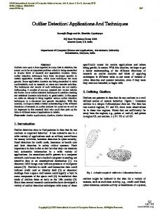
Sep 8, 2010 - creates an ordered list on the website of Netflix, called a rental queue, of movies to rent. ...... (see http://sifter.org/~simon/journal/20061211.html).
Master Thesis
Detecting unusual user profiles with outlier detection techniques
by
Martijn Onderwater
September 2010
c 2010 Martijn Onderwater
All Rights Reserved
Master Thesis
Detecting unusual user profiles with outlier detection techniques
Author: Drs. Martijn Onderwater
Supervisors: Dr. Wojtek Kowalczyk Dr. Fetsje Mon´e-Bijma
September 2010 VU University Amsterdam Faculty of Sciences De Boelelaan 1081a 1081 HV Amsterdam The Netherlands
iv
Preface The Master program Business Mathematics & Informatics at the VU University Amsterdam is concluded by an internship. My internship took place at the Fraud Detection Expertise Centre, a part of the VU University. This thesis shows the results that were obtained during the six months of the project. I would like to thank my supervisor, Wojtek Kowalczyk, for his continuous support and guidance. His practical experience and keen thinking were an inspiration, not only for finishing this thesis, but also for me personally. Finally, special thanks go to my colleagues at the Fraud Detection Expertise Centre, Rob Konijn and Vytautas Savickas, for the long discussions and useful feedback. Thanks also to Fetsje Mon´e-Bijma for reading the ‘nearly final’ version of this thesis and for providing those ever useful fresh-eyes-at-the-last-minute comments.
Martijn Onderwater, Amsterdam, the Netherlands, September 8, 2010.
v
vi
Management Summary Every year, companies worldwide lose billions of euros to fraud. Detecting fraud is therefore a key activity for many companies. But with the increasing use of computer technology and the continuous growth of companies, the amount of available data is huge. Finding fraud in such volumes of data is a challenging and time-consuming task. Automated systems are needed for these tasks. An important issue in automated fraud detection is the personal nature of user behaviour. What is normal for one person may be unusual for another. We will approach this situation by creating a so-called profile for each user. This profile is a vector of numbers that together capture important aspects of the user’s behaviour. Profiles are learned from the data, thereby eliminating the need for defining ‘normal’ behaviour and allowing for a high level of personalization. Using these profiles, we can, e.g., compare profiles and look for users with unusual behaviour. Another important advantage of profiles is that we can compare individual transactions to the user’s profile in order to determine if it conforms to normal behaviour. If the profiles are small enough to be kept in memory, transactions can be checked in real-time. Transactions can also be used to update a profile, hence making profiles evolve over time and allowing them to capture new types of fraud. In this thesis, we investigate how to create such profiles and present some techniques for comparing them. We also discuss outlier detection techniques, which can be used to find users with unusual behaviour. Dimensionality reduction techniques are presented as a method for reducing the size of a profile, which may be useful with respect to real-time processing. Special attention is paid to their effect on outliers. Throughout the thesis, experiments will be done on a practical dataset. Our main conclusion is that there is a wide variety of methods available for user profiling, outlier detection and dimensionality reduction. They can be applied in many practical situations, although the optimal choice depends highly on the application domain.
vii
viii
Contents Preface
v
Management Summary
vii
1 Introduction 1.1 Challenges . . . . . . . . . . . . . . . . . . . . . . . . . . . . . 1.2 Our approach . . . . . . . . . . . . . . . . . . . . . . . . . . . 1.3 Outline of this thesis . . . . . . . . . . . . . . . . . . . . . . . 2 The 2.1 2.2 2.3 2.4
2.5
Netflix Dataset Netflix & The Netflix Prize . . . . . . . . Description of the dataset . . . . . . . . . Creation of the dataset . . . . . . . . . . . Exploratory Data Analysis . . . . . . . . . 2.4.1 Average rating per user . . . . . . 2.4.2 Number of ratings . . . . . . . . . 2.4.3 Number of ratings per day . . . . . 2.4.4 Time between first and last rating 2.4.5 Good and bad movies . . . . . . . 2.4.6 Discussion . . . . . . . . . . . . . . Further reading . . . . . . . . . . . . . . .
. . . . . . . . . . .
. . . . . . . . . . .
. . . . . . . . . . .
. . . . . . . . . . .
. . . . . . . . . . .
3 User profiling 3.1 Profile construction . . . . . . . . . . . . . . . . . . 3.1.1 Aggregates and basic statistics . . . . . . . 3.1.2 Histograms . . . . . . . . . . . . . . . . . . 3.1.3 Modelling probability density functions . . 3.1.4 Mixture models applied to user profiling . . 3.1.5 Netflix: Simon Funk’s idea . . . . . . . . . . 3.2 Comparing profiles . . . . . . . . . . . . . . . . . . 3.2.1 Distance measures . . . . . . . . . . . . . . 3.2.2 Difference between probability distributions 3.2.3 Custom similarity measures . . . . . . . . . 3.3 Significance of the difference . . . . . . . . . . . . . ix
. . . . . . . . . . .
. . . . . . . . . . .
. . . . . . . . . . .
. . . . . . . . . . .
. . . . . . . . . . .
. . . . . . . . . . .
. . . . . . . . . . .
. . . . . . . . . . .
. . . . . . . . . . .
. . . . . . . . . . .
1 2 3 3
. . . . . . . . . . .
5 5 6 7 9 9 10 11 13 13 15 15
. . . . . . . . . . .
17 17 18 18 19 23 25 27 27 28 30 31
CONTENTS
3.4 3.5
Discussion . . . . . . . . . . . . . . . . . . . . . . . . . . . . . Further reading . . . . . . . . . . . . . . . . . . . . . . . . . .
31 31
4 Outlier Detection 4.1 Statistics-based techniques . . . . . . . . . 4.1.1 One dimensional data . . . . . . . 4.1.2 Robust Least Squares . . . . . . . 4.2 Distance-based techniques . . . . . . . . . 4.2.1 Onion Peeling . . . . . . . . . . . . 4.2.2 Peeling with standardized data . . 4.2.3 Peeling with Mahalanobis distance 4.2.4 Local Reconstruction Weights . . . 4.3 Experiments . . . . . . . . . . . . . . . . . 4.4 Discussion . . . . . . . . . . . . . . . . . . 4.5 Further reading . . . . . . . . . . . . . . .
. . . . . . . . . . .
. . . . . . . . . . .
. . . . . . . . . . .
. . . . . . . . . . .
. . . . . . . . . . .
. . . . . . . . . . .
. . . . . . . . . . .
. . . . . . . . . . .
. . . . . . . . . . .
. . . . . . . . . . .
. . . . . . . . . . .
33 33 33 34 35 35 35 36 36 36 37 38
5 Dimensionality reduction techniques 5.1 Principal Component Analysis . . . . . 5.2 Multidimensional Scaling . . . . . . . . 5.3 AutoEncoders . . . . . . . . . . . . . . . 5.4 Locally Linear Embedding . . . . . . . . 5.5 t-Stochastic Neighbourhood Embedding 5.6 Discussion . . . . . . . . . . . . . . . . . 5.7 Further reading . . . . . . . . . . . . . .
. . . . . . .
. . . . . . .
. . . . . . .
. . . . . . .
. . . . . . .
. . . . . . .
. . . . . . .
. . . . . . .
. . . . . . .
. . . . . . .
. . . . . . .
41 42 43 44 46 47 48 49
. . . . . . .
6 Detecting change in behaviour 51 6.1 Histogram profiles . . . . . . . . . . . . . . . . . . . . . . . . 51 6.2 Funk profiles . . . . . . . . . . . . . . . . . . . . . . . . . . . 55 6.3 Further reading . . . . . . . . . . . . . . . . . . . . . . . . . . 56 7 Conclusions and recommendations 59 7.1 Conclusions . . . . . . . . . . . . . . . . . . . . . . . . . . . . 59 7.2 Recommendations . . . . . . . . . . . . . . . . . . . . . . . . 60 A Visualising good and bad movies
63
B Matlab: odToolbox 67 B.1 Available scripts . . . . . . . . . . . . . . . . . . . . . . . . . 67 B.2 Demo script . . . . . . . . . . . . . . . . . . . . . . . . . . . . 68 Bibliography
75
x
Chapter 1
Introduction Outlier detection refers to the problem of finding patterns in data that do not conform to expected behaviour. Depending on the application domain, these non-conforming patterns can have various names, e.g., outliers, anomalies, exceptions, discordant observations, novelties or noise. The importance of outlier detection methods is found in the fact that the results can lead to actionable (and often critical) information. A good example of this is fraud detection, where an outlier can indicate, e.g., a suspicious credit card transaction that needs to be investigated. The amount of money involved in fraud is enormous. Sudjianto et al. (2010) estimate the amount of credit card fraud in the US at $1 billion per year and $10 billion worldwide. In the United Kingdom The UK Card Association and Financial Fraud Action UK publish a yearly report on plastic card fraud. They report an amount of £440 million for the year 2009 (UKCards (2010)). These statistics are only about card fraud, but there are many other areas where fraud exists, such as: • Health care. Health care providers declaring costs for services that were never provided. • Public transport. Copying of payment cards used to pay for public transport. • Insider trading. Certain transactions on a financial market may be suspicious because they suggest insider trading. • Social welfare. People receiving benefits which they are not entitled to. • Telecommunications. Detecting cloned phones (superimposition fraud). 1
CHAPTER 1. INTRODUCTION
Together these industries face massive amounts of fraud, a part of which can be detected by outlier detection methods. Besides fraud detection, there are many other areas where outlier detection methods (can) play a role: • Intrusion detection. Detecting unauthorized access to computer networks. • Loan application processing. Identifying potentially problematic customers. • Motion segmentation. Detecting image features moving independently from the background. • Environmental monitoring. Predicting the likelihood of floods, fire or draught based on environmental data. More examples can be found in Hodge and Austin (2004) and Zhang et al. (2007).
1.1
Challenges
At an abstract level, an outlier is defined as a pattern that does not conform to normal behaviour. A straightforward outlier detection approach, therefore, is to define a region representing normal behaviour and declare any observation in the data that does not belong to this region as an outlier. But several factors make this difficult (from Chandola et al. (2009)): • Defining a normal region which encompasses every possible normal behaviour is very difficult. Especially since ‘normal’ is something that depends very much on the user. • Criminals continually adapt their behaviour to fraud detection techniques, trying to make fraudulent transactions appear normal again. So both fraud and the detection techniques change over time in response to each other. • Outlier detection techniques are often partly domain-specific, making it difficult to port existing techniques to other domains. • Existing outlier detection techniques are often aimed at finding outliers in one big dataset. In the context of fraud, we are more interested in identifying outliers per user, for whom fewer records are available. This makes applying conventional techniques difficult. 2
CHAPTER 1. INTRODUCTION
• Labelled data is often sparse, making it difficult to use classic supervised classifiers. • The data often contains some noise, such as typos. This noise usually appears among the outliers. • The amount of data available is usually quite large and decisions about being an outlier or not need to be taken in real-time. This happens with, e.g., credit card transactions, which need to be blocked when they appear suspicious.
1.2
Our approach
We will approach the situation by creating a so-called profile for each user. This profile is a vector of numbers that together capture important aspects of the user’s behaviour. Profiles are learned from the data, thereby eliminating the need for defining ‘normal’ behaviour. By comparing profiles we can find users with unusual behaviour. Such profiles are very relevant in the context of fraud detection. An incoming transaction of a user can be compared to the user’s profile in order to determine if it conforms to normal behaviour. If the profiles are small enough to be kept in memory, transactions can be checked in real-time. Transactions can also be used to update a profile, hence making profiles evolve over time and allowing them to capture new types of fraud. The dataset that we use is large and unlabelled, as is often the case in practice. With respect to outliers, we will limit ourselves to detecting them. We will not give a practical explanation for why they are outliers, because that task is very domain specific and we lack the domain knowledge and expertise. As a consequence, we also will not judge whether an outlier is noise. It is our intention to investigate techniques for user profiling and outlier detection and to apply these techniques to detect change in user behaviour. We will also provide a collection of Matlab tools for future use within the Fraud Detection Expertise Centre.
1.3
Outline of this thesis
The next chapter of this thesis introduces the dataset that we will use and does some exploratory data analysis to get a feel for the data. Chapter 3 shows how profiles can be constructed from this data and compared. In chapter 4 we investigate existing outlier detection methods and apply them 3
CHAPTER 1. INTRODUCTION
to some profiles. Chapter 5 contains experiments with several dimensionality reduction techniques in order to find out if (and how) useful low dimensional representations of the data are. Then in chapter 6 we apply some of the outlier detection techniques from chapter 4 to detect changes in user behaviour over time. We finish the thesis with an overview of conclusions and some recommendations for further research. All our experiments will be done in Matlab, with the occasional help of Java and C++ (via Matlab’s external interfaces), on a computer with two quad-core processors and 16GB of internal memory. Not all the computing power of that machine is necessary for all experiments, but a dual-core machine with at least 4GB of memory is advisable for the dataset that we use.
4
Chapter 2
The Netflix Dataset 2.1
Netflix & The Netflix Prize
The dataset that we will use is obtained from Netflix. They provide a monthly flat-fee service for the rental of DVD and Blu-ray movies. A user creates an ordered list on the website of Netflix, called a rental queue, of movies to rent. The movies are delivered individually via the United States Postal Service. The user can keep the rented movie as long as desired, but there is a limit on the number of movies (determined by subscription level) that each user can have on loan simultaneously. To rent a new movie, the user must mail the previous one back to Netflix in a prepaid mailing envelope. Upon receipt of the disc, Netflix ships the next available disc in the user’s rental queue. After watching the movie, the user can give it a rating from one to five on the Netflix website. Netflix has a recommender system (Cinematch) that uses these ratings to suggest other movies that may be interesting for the user. In October 2006, Netflix started a competition to see if and how the predictions of Cinematch could be improved. A dataset of 100.480.507 ratings that 480.189 users gave to 17.770 movies was made publically available and the research community was invited to join the competition. The grand prize was $1.000.000 for the first team to improve Cinematch by 10%. Also, a yearly progress prize of $50.000 was awarded to the team that made the most progress. In September 2009, team BellKor’s Pragmatic Chaos, a cooperation of people with previous success in the competition, won the competition and received the grand prize. They narrowly beat team The Ensemble, who also managed to improve Cinematch by 10%, but performed slightly worse on a test set.
5
CHAPTER 2. THE NETFLIX DATASET
There have been some complaints and concerns about the competition. Although the datasets were changed to preserve customer privacy, the competition has been criticized by privacy advocates. In 2007 two researchers from the University of Texas (Narayanan and Shmatikov (2006)) were able to identify individual users by matching the datasets with film ratings on the Internet Movie Database (www.imdb.com). In December 2009, an anonymous Netflix user sued Netflix, alleging that Netflix had violated U.S. fair trade laws and the Video Privacy Protection Act by releasing the datasets. Due to these privacy concerns, Netflix decided not to pursue a second competition. Also, the dataset is currently not available to the public any more. The announcement by Netflix to cancel the second competition can be found at http://tiny.cc/br3tx. A response by the researchers from the University of Texas is also online, see http://33bits.org/2010/03/15/open-letter-to-netflix/. More references can be found in section 2.5.
2.2
Description of the dataset
The dataset contains 100.480.507 pairs of . For users we have only their ID, but for movies we also have a title and the year of release. We use this dataset1 because it is close to the challenges described in section 1.1 and our approach to the problem. More specific: • The total dataset, which is about 2GB in size, gives us computational problems similar to those encountered in practice. • The dataset contains ratings, so with respect to predicting ratings the dataset is labelled. But we can also treat the ratings as another attribute in the dataset. This makes the dataset unlabelled, which is again similar to practical situations. • There are ratings from 480.189 users, enough for defining user profiles and looking for outliers among them. • There were 51051 competitors in 41305 teams participating in the Netflix Prize competition. During the three years of the competition, 1
Initially, we intended to use data from a customer of the Fraud Detection Expertise Centre. Unfortunately, for bureaucratic reasons, permission for using the data was never given. As an alternative, we decided to use the Netflix data, for the reasons outlined in this section.
6
CHAPTER 2. THE NETFLIX DATASET
the ideas and solutions of participants were actively discussed on, e.g., the Netflix Prize forum. Because of this, the dataset is well understood. This forum can be found online at http://www.netflixprize.com/community. • There are only a few attributes in the dataset, so we do not need to spend time understanding attributes, identifying important attributes and other such considerations. This allows us to focus on the problem.
2.3
Creation of the dataset
When the competition started, Netflix made four datasets available to the public: • Training set. This is the dataset that participants of the competition used to train their models. • Qualifying set. The dataset containing pairs for which the ratings had to be predicted. • Probe set. This dataset is a subset of the training set and could be used by teams for testing their models. • Quiz set. A subset of the qualifying set. Submissions were judged on this subset. • Test set. Another subset of the qualifying set, used to rank submissions that had equal results on the quiz set. The dataset that we described above is the trainingset. The way in which these sets were sampled from Netflix’ systems was described in the rules and in a later post on the forum. Below is a quote from the forum (see http://www.netflixprize.com/community/viewtopic.php?id=332 for the full post). We first formed the complete Prize dataset (the training set, which contains the probe subset, and the qualifying set, which comprises the quiz and test subsets) by randomly selecting a subset of all our users who provided at least 20 ratings between October, 1998 and December, 2005 (but see below). We retrieved all their ratings. We then applied a perturbation technique to the ratings in that dataset. The perturbation technique was designed not to change the overall statistics of the Prize dataset. However, we will not describe the 7
CHAPTER 2. THE NETFLIX DATASET
perturbation technique here since that would defeat its purpose of protecting some information about the Netflix customer base. As described in the Rules, we formed the qualifying set by selecting, for each of the randomly selected users in the complete Prize dataset, a set of their most recent ratings. These ratings were randomly assigned, with equal probability, to three subsets: quiz, test, and probe. Selecting the most recent ratings reflects our business goal of predicting future ratings based on past ratings. The training set was created from all the remaining (past) ratings and the probe subset; the qualifying set was created from the quiz and test subsets. The training set ratings were released to you; the qualifying ratings were withheld and form the basis of the Contest scoring system. Based on considerations such as the average number of ratings per user and the target size of the complete Prize dataset, we selected the user’s 9 most recent ratings to assign to the subsets. However, if the user had fewer than 18 ratings (because of perturbation), we selected only the most recent one-half of their ratings to assign to the subsets. There was a follow-up post with two additional remarks about this process: First, we stated that the ratings were sampled between October, 1998 and December, 2005, but the earliest recorded date is 11 November 1999. The code to pull the data was written to simply ensure the rating date was before 1 January 2006; we assumed without verifying that ratings were collected from the start of the Cinematch project in October 1998. In fact, the earliest recordings of customer ratings in production date from 11 November 1999. Second, we reported that we included users that had only provided at least 20 ratings. Unfortunately a bug in the code didn’t require the ratings to have made before 1 January 2006. Thus the included users made at least 20 ratings through 9 August 2006, even if all ratings made after 1 January 2006 are not included. This last remark is phrased somewhat cryptic. We look at the number of ratings per user in section 2.4.2, so the situation with respect to the training set will become clear there. See also the section called The Prize Structure in the rules of the competition at http://www.netflixprize.com/rules. 8
CHAPTER 2. THE NETFLIX DATASET
2.4
Exploratory Data Analysis
Before we start working with, e.g., user profiling and outlier detection, we do some exploratory data analysis on the dataset. This helps us to get a feel for the data and see if certain aspects of it conform to our expectations. The analysis is not a fixed list of steps to take, but rather a creative process where common sense and some simple statistics are combined. In practice, the knowledge obtained from such experiments is often important when interpreting results later on in the project. It also raises the level of domain knowledge of the (often externally hired) data analyst early on in the project. The following sections contain a selection of the results of our exploratory data analysis.
2.4.1
Average rating per user
It seems natural to assume that most users will watch more movies that they like than movies that they do not like. Hence, the average rating should be just above three for most users. The left of figure 2.1 shows a histogram of these averages. As can be seen, most users do indeed have an average rating of just above three. There are some users that have a very low or high average and we suspect those users have only rated a few movies. If we leave such users out and recalculate the histogram for users that have at least, say, 100 ratings, we get the histogram that is shown in the right part of figure 2.1.
Figure 2.1: Left: histogram of the average rating per user of all 480189 users. Right: histogram of the average rating per user of the (234909) users that rated more than 100 movies. 9
CHAPTER 2. THE NETFLIX DATASET
Note that there are still users with very low and very high rating. An example of such a user is user 2439493, who rated 16565 movies. A histogram of this user’s ratings is shown in figure 2.2. Over 90% of these ratings were a one. Histogram of the ratings of user 2439493 16000 14000 12000
Counts
10000 8000 6000 4000 2000 0
1
2
3 Rating
4
5
Figure 2.2: Histogram of ratings of user 2439493.
2.4.2
Number of ratings
We already saw that there are some users who have only a few ratings. Figure 2.3 shows the number of ratings done by each user. For clarity, they are sorted by the amount of ratings.
Figure 2.3: Number of ratings per user (sorted by number of ratings). 10
CHAPTER 2. THE NETFLIX DATASET
The plot shows a sharp peak on the left, indicating that there are only a few users with a large number of ratings (compared to the others). The plot on the right zooms in on the peak, showing that there are only about 5 users with more than 10000 ratings. A closer examination of the data tells us that there are 1212 users with more than 2000 ratings and 16419 users with less than 10 ratings. Another plot that gives some insight into the activity of users can be created by plotting the cumulative sum of the data in figure 2.3 and scaling it to make the total sum equal to one. The result is in figure 2.4, from which it can be seen directly that 70% of the ratings is done by approximately the 120000 most active users. Cumulative and scaled #ratings (70 % of ratings done by top 118532 users) 1 0.9 0.8
Cumulative scaled counts
0.7 0.6 0.5 0.4 0.3 0.2 0.1 0
0
0.5
1
1.5
2
2.5 Users
3
3.5
4
4.5
5 5
x 10
Figure 2.4: Number of ratings per user, sorted by number of ratings, summed cumulatively and normalized to one.
2.4.3
Number of ratings per day
The Netflix data contains ratings from 11 November 1999 to 31 December 2005, so roughly six years. At the beginning of this period, Netflix was not a big company and use of the internet was only just getting popular. So the number or rating should be small there. But after that, the number of 11
CHAPTER 2. THE NETFLIX DATASET
ratings should grow steadily. It would be interesting to see what happened in, say, the last two years. Is Netflix’ popularity still growing? Figure 2.5 shows the number of ratings per day. 5
8
x 10
#ratings per day, from 11−Nov−1999 to 31−Dec−2005.
7 6
# ratings
5 4 3 2 1 0
0
500
1000
1500
2000
2500
Time
Figure 2.5: Number of ratings per day. The number of ratings per day is indeed low in the beginning and growing as time goes on. But near the end of the period it seems to drop a bit. Also, there is a sharp peak, which turns out to be the 29 January 2005. Both facts could be caused by the fact that the dataset is only a sample of all the data in Netflix’ system. The sampling was not done with the number of ratings per day in mind (see section 2.3). For the peak on 29 January 2005, there may be some other causes. For instance: • Automatic script. It may have been that somebody wrote an automatic script to do a lot of ratings. Our analysis does not show any evidence of this. The ratings on 29 January 2005 were done by a multitude of users. Also, the ratings were distributed similar to the histograms in figure 2.1, so they appear to be valid ratings. • System crash. Perhaps a system crashed at Netflix somewhere before 29 January 2005 and they used this day to reinsert some lost data. But this would mean that there should be a decrease of the number of ratings in the days before 29 January 2005. A closer look at the data does not show such a decrease. • Holiday. 29 January 2005 is not a special day like Christmas or Thanksgiving, where we can expect an increase in number of ratings. 12
CHAPTER 2. THE NETFLIX DATASET
So all in all we are confident that the ratings on 29 January 2005 are valid. There is also a discussion on the Netflix forum about the ratings of this day, see the topic at http://www.netflixprize.com/community/viewtopic.php?id=141.
2.4.4
Time between first and last rating
It seems natural to interpret the time between the first and last rating as the membership period of a user. Figure 2.6 shows a histogram of how many users have been a member for how many months. Its shape is as expected, with mainly recent members and some long-time members. We also investigated whether there was a correlation between the number of ratings of a user and the length of its membership, but found no significant relation. This is probably the result of the perturbation method. Because of this, we should probably not interpret the time between the first and last rating as the membership period of a user.
4
3
Histogram of #user vs #months of membership.
x 10
2.5
#Users
2
1.5
1
0.5
0
0
10
20
30
40 Months
50
60
70
80
Figure 2.6: Histogram of the membership time (in months) of the users.
2.4.5
Good and bad movies
It is interesting to investigate whether our intuition of a ‘good’ and ‘bad’ movie is reflected in the data. For instance, we expect that movies with a large number of ratings and a large average are good movies. Similarly, bad movies are expected to have a low average and only a few ratings. 13
CHAPTER 2. THE NETFLIX DATASET
Applying this to the Netflix data results in the movies in tables 2.1 and 2.2. The good movies are found by looking for movies with more than 5000 ratings and selecting the ones with the highest average rating. The titles in table 2.1 are recognizable as known blockbusters or very popular TV-series. Pos. 1. 2. 3. 4. 5. 6. 7. 8. 9. 10.
Title LOTR2 : The Return of the King (2003) LOTR: The Fellowship of the Ring (2001) LOTR: The Two Towers: (2002) Lost: Season 1 (2004) The Shawshank Redemption (1994) Arrested Development: Season 2 (2004) The Simpsons: Season 6 (1994) Star Wars: V: The Empire Strikes Back (1980) The Simpsons: Season 5 (1993) The Sopranos: Season 5 (2004)
Average 4.7233 4.7166 4.7026 4.6710 4.5934 4.5824 4.5813 4.5437 4.5426 4.5343
# ratings 73335 73422 74912 7249 139660 6621 8426 92470 17292 21043
Table 2.1: Good movies. The bad movies are found by looking for movies with the lowest average rating. Table 2.2 shows very few known titles, although Zodiac Killer (2004) appears on the IMDB bottom 100 list at position 30. See http://www.imdb.com/chart/bottom. Also, the makers of The Worst Horror Movie Ever Made (2005) came very close to reaching their target. Pos. 1. 2. 3. 4. 5. 6. 7. 8. 9. 10.
Title Avia Vampire Hunter (2005) Zodiac Killer (2004) Alone in a Haunted House (2004) Vampire Assassins (2005) Absolution (2003) The Worst Horror Movie Ever Made (2005) Ax ’Em (2002) Dark Harvest 2: The Maize (2004) Half-Caste (2004) The Horror Within (2005)
Average 1.2879 1.3460 1.3756 1.3968 1.4000 1.4000 1.4222 1.4524 1.4874 1.4962
# ratings 132 289 205 247 125 165 90 84 119 133
Table 2.2: Bad movies. Note that table 2.2 contains quite recent movies that have not all had the time to reach their ‘long-term’ average (the Netflix data only contains 2
LOTR=Lord of the Rings
14
CHAPTER 2. THE NETFLIX DATASET
ratings from the years 2000 to 2005). If we define bad movies as those with low average, but with a decent amount of ratings, then we expect to see more recognizable bad titles. Table 2.3 shows movies with the lowest average among those with at least 1000 ratings. The titles are indeed more recognizable. Pos. 1. 2. 3. 4. 5. 6. 7. 8. 9. 10.
Title Shanghai Surprise (1986) Sopranos Unauthorized: Shooting Sites Uncovered (2002) Gigli (2003) House of the Dead (2003) Glitter (2001) National Lampoon’s Christmas Vacation 2 (2003) Stop! Or My Mom Will Shoot (1992) Druids (2001) Wendigo (2002) The Brown Bunny (2004)
Average 1.7626 1.9375
# ratings 1192 1104
1.9460 1.9628 1.9665 1.9712
9958 5589 2596 1387
1.9747 2.0185 2.0619 2.0684
2215 1297 1066 3814
Table 2.3: Bad movies with at least 1000 ratings.
2.4.6
Discussion
Based on the analysis we can say that the data does contain some outliers, both in terms of the number of ratings and the distribution of ratings. So we will expect some results from the work on user profiling and outlier detection in the next few chapters. The data does not seem to contain any strange phenomena that can somehow cause us problems later on.
2.5
Further reading
More information on Netflix and the Netflix Prize can be found the following webpages: • Netflix’ homepage, http://www.netflix.com. • Homepage of the Netflix Prize, http://www.netflixprize.com/. It also has a forum where the competition was discussed by the community. The forum is read-only since the cancellation of the second Netflix Prize. • The Wikipedia page for Netflix (http://en.wikipedia.org/wiki/Netflix) and the Netflix Prize (http://en.wikipedia.org/wiki/Netflix_Prize). These are the main sources for the information in section 2.1. 15
CHAPTER 2. THE NETFLIX DATASET
There have been many papers on the Netflix Prize, see, e.g., Bell and Koren (2007a), Bell and Koren (2007b), Takacs et al. (2007), Paterek (2007) and Bennett and Lanning (2007). Also, the four top competitors presented their techniques at the 2009 KDD conference. See www.kdd.org for the papers. An alternative to the Netflix dataset is the MovieLens dataset. Both are similar in nature, but the MovieLens dataset contains fewer records and more information on users and movies. It can be downloaded from www.grouplens.org. With respect to recommender systems, papers by Mobasher et al. (2007) and Williams et al. (2007) are worth mentioning. They investigate methods of attack on recommender systems and techniques for preventing such attacks. The histogram of user 2439493 in figure 2.2 is an example of such an attack. Over 90% of his/her 16565 ratings were a one, which is highly suspicious.
16
Chapter 3
User profiling We would like to construct profiles that can capture the ‘behaviour’ of a user from his transactions in the past. That way, we can monitor the change in these profiles and raise a warning when the change is significant. The most common interpretation is that a profile consists of elements, where each element captures one aspect of the user’s behaviour. Typically, an element is a number or a group of numbers. In the context of credit card transactions, elements of a profile could be, e.g., • the daily number of transactions; • the average amount of money spent per day/week/month; • a histogram (or quantiles) describing the distribution of the daily number of transactions. There are four important issues related to the problem of user profiling: 1. How to choose the numbers or groups of numbers that make up the profile? 2. How to compare profiles and how to quantify the difference? 3. How to determine if a difference is significant? We will discuss these issues in this chapter.
3.1
Profile construction
Usually, experts with domain knowledge already have a good idea which aspects of a user’s behaviour are important for detecting outliers. So in practice we ‘only’ need to determine how to represent these aspects as elements in a profile. Note that there is no ‘universal’ good or bad way of 17
CHAPTER 3. USER PROFILING
constructing the profiles; it depends very much on the domain. In the following sections, we will describe some elements in the context of the Netflix data. They are intended as examples of what is possible.
3.1.1
Aggregates and basic statistics
The list below contains some of the profile elements used by The Ensemble, the runner-up in the Netflix Prize competition. See Sill et al. (2009). The exact meaning of these elements is not important, but it should make clear that defining them is a creative process where one learns by trial and error. • A binary variable indicating whether the user rated more than 3 movies on this particular date. • The logarithm of the number of distinct dates on which a user has rated movies. • The logarithm of the number of user ratings. • The mean rating of the user, shrunk in a standard Bayesian way towards the mean over all users of the simple averages of the users. • The standard deviation of the date-specific user means from a model which has separate user means (a.k.a. biases) for each date. • The standard deviation of the user ratings. • The logarithm of (rating date - first user rating date + 1). • The logarithm of the number of user ratings on the date + 1.
3.1.2
Histograms
For the Netflix dataset, we could use a histogram of the ratings done by a particular user as his/her profile. This histogram can then be either normalized to have total area one or left unnormalized (with counts in the histogram). For instance, the unnormalized histogram profile of user 2439493 was already shown in figure 2.2 in section 2.4.1. The normalized histogram of user 42 is shown in figure 3.1. 18
CHAPTER 3. USER PROFILING
Scaled histogram of the ratings of user 42 1 0.9 0.8
Relative frequency
0.7 0.6 0.5 0.4 0.3 0.2 0.1 0
1
2
3 Rating
4
5
Figure 3.1: Histogram of ratings of user 42.
3.1.3
Modelling probability density functions
Here, we take a more probabilistic approach to the problem and try to find a probability density function (p.d.f.) that models the user’s behaviour well. This way, the profile can consist of only the parameter(s) of this p.d.f. In simple situations, we can use one of the known distributions (Normal, Log-Normal, multinomial, Poisson, . . .) and fit it to the user’s data. But usually it is unknown which of these distributions fits the data best and we need to use other techniques. The most common approach is to use a so-called Mixture Model, which models the user’s behaviour as a weighted sum of p.d.f.’s. The weighted sum is created in such a way that the Mixture Model is again a p.d.f. By using this Mixture Model, we can model p.d.f.’s of a more general form than those covered by the classical p.d.f.’s. The payoff is that more parameters need to be kept in the profile, as well as the weights. Below we will discuss some examples of Mixture Models that are commonly used. Section 3.5 contains some more references on modelling p.d.f.’s. Mixture of Gaussians This is one of the most common approaches of modelling p.d.f.’s and is usually denoted by GMM (Gaussian Mixture Model). Generally speaking, we assume that records in the dataset are generated from a (weighted) 19
CHAPTER 3. USER PROFILING
mixture of K Gaussian distributions, i.e., p(y) =
K X
αk · pk (y; µk , Σk ).
k=1
The µk and Σk are the parameters of the K Gaussian distributions pk and the αk are weights such that K X
αk = 1,
αk > 0
∀k = 1 . . . K.
k=1
See also the textbooks by Bishop (2007) and Duda et al. (2000). The µk , Σk and αk are to be learned from the data. Learning is done with the help of the Expectation-Maximization algorithm (EM in short) by Dempster et al. (1977): Algorithm 1: Expectation-Maximization (applied to GMM). 1. Start with some initial values for the parameters and weights. A common approach is to initialize αk , µk and Σk with the results of a few iterations of K-means. 2. E-step: For each data point y, calculate the membership probability pk (y; µk , Σk ) of each component k. 3. M-step: For each component k, find the points for which this component is the one with the highest membership probability. Based on these points, re-estimate µk and Σk . Update αk to the fraction of all points that is in component k. 4. Repeat steps 2 and 3 until convergence or until a number of predefined iterations has been done.
Mixture of multinomials Another option is to model p.d.f.’s via a mixture of multinomials. Where GMM’s are for continuous data, multinomials can be used for discrete data. The p.d.f. of a d-dimensional multinomial distribution is given by �Y d N θiyi , y1 · . . . · yd
� p(y; θ) =
(3.1)
i=1
where N = y1 + . . . + yd and the parameters θ satisfy θ1 + . . . θd = 1. A mixture of multinomials then becomes 20
CHAPTER 3. USER PROFILING
p(y) =
K X
αk pk (y; θ),
k=1
with pk (y; θ) as in equation (3.1) and again K X
αk = 1,
αk > 0
∀k = 1 . . . K.
k=1
As with Gaussian Mixture Models, estimation of the parameters can be done with EM. Algorithm 2 shows the procedure. Algorithm 2: Learning a mixture of multinomials. 1. Initialize parameters θk randomly and weights to, e.g., αk =
1 K.
2. E-step: For each data point y, calculate the membership probability pk (y; θk ) of each component k. 3. M-step: For each component k, find the points for which this component is the one with the highest membership probability. Based on these points, re-estimate θk . Update αk to the fraction of all points that is in component k. 4. Repeat steps 2 and 3 until convergence or until a number of predefined iterations has been done.
During the calculation of the membership probabilities (from equation (3.1))in the E-step, the multinomial coefficient is usually omitted. This can be done because the coefficient is the same for all components and thus has no influence on the M-step.
Naive Bayes Estimation This technique by Lowd and Domingos (2005) combines the previous two ideas and uses Gaussians for continuous attributes and multinomials for discrete attributes. What is special about this algorithm is that it also tries to estimate the number of components that are needed in the mix by repeatedly adding and removing components. The procedure is shown in algorithm 3. It takes as input: a training set T, a hold-out set H, the number of initial components k0 and the convergence thresholds δEM and δADD . 21
CHAPTER 3. USER PROFILING
Algorithm 3: Naive Bayes Estimation (by Lowd and Domingos (2005)). Initialise the mixture M with one component. Set k = k0 and Mbest = M . Repeat:
Add k new components to M and initialise them with k random samples from T. Remove these samples from T. Repeat:
E-step: Calculate the membership probabilities. M-step Re-estimate the parameters of the mixture components. Calculate log(p(H|M )). If it is the best so far, set Mbest = M . Every 5 iterations of EM, prune low-weight components. Until:log(p(H|M )) fails to improve by more than δEM .
M ← Mbest . Prune low-weight components. k ← 2k. Until:log(p(H|M )) fails to improve by more than δADD .
Apply EM twice more to Mbest with both H and T.
Note that each time the EM algorithm converges on a mixture, the procedure doubles the amount of components to add to the previous mixture. This is counter balanced by the periodic pruning of low-weight components. The authors compare NBE to Bayesian Networks (using Microsoft Research’s WinMine Toolkit) by applying them to 50 datasets. They find that both methods give comparable results. Our experiments with this algorithm suggest some aspects that are a candidate for improvement: • Merging components. NBE does not merge similar components, only components that have exactly the same parameters. As a result, NBE often returns mixtures with very similar components. 22
CHAPTER 3. USER PROFILING
• Extra EM iterations. NBE finishes with two extra EM iterations on Mbest . Our experiments show that it is usually wise to do more of these iterations instead of adding more components.
3.1.4
Mixture models applied to user profiling
A very nice example of learning mixture models as user profiles is given in a paper by Cadez et al. (2001). There they deal with a department store that has collected data about purchases of customers. Cadez et al. (2001) are interested in creating a customer profile that captures the amount of products that a customer buys in one transaction in each of the store’s 50 different departments (its ‘behaviour’). Their approach is as follows: • Create a ‘global profile’ that captures the behaviour of the ‘average’ user. It is a mix of 50-dimensional multinomials, learned from all transactions of all customers. • Personalize this global profile to a customer profile. This is done by ‘tuning’ the weights in the global profile to customer-specific weights, based on the transactions of the customer. These customer-specific weights then form a customer profile. The global profile is learned using algorithm 2 from section 3.1.3. To formalize this, we need some notation. The data consists of individual transactions yij , indicating the jth transaction of customer i. Each yij is a vector (of length 50) of the number of purchases per department. Supposing that transaction yij is generated by component k, the probability of transaction yij (its ‘membership probability’) is p(yij |k) ∝
C Y
n
θkcijc ,
(3.2)
c=1
where 1 ≤ c ≤ C is the department number (C = 50), θk∗ are the 50 parameters of the kth multinomial and nijc is the number of items bought in transaction yij in department c. Note that the parameters θkc of the components in the mixture do not depend on customer i: they are global. Also observe that the multinomial coefficient is omitted (as remarked after algorithm 2), hence the ’∝’ in equation (3.2). The probability of transaction yij now becomes p(yij ) =
K X
αk p(yij |k).
k=1
The αk are the weights (with total sum 1). Algorithm 2 can now be applied using equations 3.2 and 3.3. 23
(3.3)
CHAPTER 3. USER PROFILING
Personalising the global weights αk to customer-specific weights αik is done by applying one more iteration of EM using only the transactions of a customer. There are also other options for obtaining customer-specific weights, see the appendix in Cadez et al. (2001). Once the αik are known, the p.d.f. describing the customer’s behaviour is given by
p(yij ) =
K X
αik p(yij |k).
(3.4)
k=1
The paper by Cadez et al. (2001) also provides some figures illustrating the technique described above. Figure 3.2 shows a histogram of the components in the global profile after learning a mixture of K = 6 multinomials from all the transactions. Note that each component has most of its probability mass before or after department 25. The components capture the fact that the departments numbered below 25 are men’s clothing and the ones numbered above 25 are women’s clothing.
Figure 3.2: Global model: histogram of each of the K = 6 components. 24
CHAPTER 3. USER PROFILING
Figure 3.3: Histogram of the global components combined with the global weights (top) and the customer-specific weights (bottom). The authors also show the effect of the extra EM iteration for learning customer-specific weights. For this, they select a customer who purchased items in some of the departments 1-25, but none in the departments higher than 25. The bottom half of figure 3.3 shows a histogram of the ‘personalized mixture’ of equation 3.4 (the global components combined with the customer-specific weights). For comparison, the top half of figure 3.3 shows a histogram of the components combined with the global weights. Note that, in the bottom half of figure 3.3, there is some probability mass in departments higher than 25, even though this customer never bought anything there. The model has learned from the global components that it happens sometimes that people shop for both men’s and women’s clothes and has incorporated this knowledge in the customer’s behaviour.
3.1.5
Netflix: Simon Funk’s idea
There are many other ideas that can be used to obtain profiles or profile elements. With respect to the Netflix data, one such example was given by Simon Funk, a pseudonym for Brandyn Webb. In december 2006 he reached third place and published his approach to the problem on his blog (see http://sifter.org/~simon/journal/20061211.html). DeSetto and DeSetto (2006) implemented this idea and made C++ code publically available. Simon Funk’s idea is based on the Singular Value Decomposition of a matrix. This method states that every n × m matrix X can be decomposed into three matrices U (n × n), D (n × m) and V (m × m) such that 25
CHAPTER 3. USER PROFILING
X = U DV T . Here, U and V are unitary matrices and D is a rectangular diagonal matrix. The entries on the main diagonal of D are called the singular values. In theory, SVD could be applied to the ratings matrix R, the matrix of size #users × #movies with ratings as entries. The number of values in this matrix is 480.189 · 17.770 = 8.532.958.530. With such numbers, R would use about 7GB of memory and the matrix U would take about 850GB. So the matrices are too big to use in this way. Also, the Netflix dataset does not contain ratings of all users for all movies, so most of the entries in R are unknown. So before applying SVD, we would need to substitute the unknown ratings by, e.g., zero or a random value. This is an extra source of errors and, because of the many missing values, probably a big source. Funk’s idea continues along this line and provides a solution for both the size of the matrices and the missing values. He suggests to create ‘features’ of length f for both movies and users in such a way that the predicted rating of user i for movie j is given by rˆij =
f X
uik · mjk .
(3.5)
k=1
Here, (ui1 , . . . , uif ) and (mj1 , . . . , mjf ) are the user and movie features respectively. He then defines the error function E=
X
(ˆ rij − rij )2 ,
i,j
which is a function of all the movie and user features, so (480.189 + 17.770) · f unknowns in total. A minimum of this function can then be found be applying gradient descent. The number of features f is determined experimentally (f ≈ 100 for the Netflix data). Note that, if all user had rated all movies, equation (3.5) would be equivalent to decomposing R in matrices U (n × f ) and M (m × f ) such that R = UMT . Up to some constant factors this is equivalent to SVD, which explains the relation to SVD. But note that Funk’s idea only uses the known ratings and is computationally inexpensive, both big advantages compared to the SVD approach. Because of these properties, as well as its simplicity, clear 26
CHAPTER 3. USER PROFILING
practical interpretation and accuracy, Funk’s idea became a prominent algorithm in the Netflix Prize competition. We modified the code by DeSetto and DeSetto (2006) slightly so that it is useable in Matlab. To keep computations time within acceptable bounds, we limit the algorithm to f = 6 features. For each user (and each movie) this results in a vector of 6 numbers, which we refer to as Funk’s (user) profile in the rest of this thesis. As an example, we take user 42 for whom we saw the histogram profile in figure 3.1. This user has profile 1.7690
-0.4779
0.1619
-0.0178
0.1611
-0.1770
Another example is user 2439493 (from figure 2.2) who has profile 0.1458
-0.4505
0.2748
-0.1985
-0.3632
-0.0764
Note that, with respect to user profiling, we do not know which aspects of user behaviour are captured by these numbers. We only know that they can be combined with features of a movie to predict the user’s rating of that movie.
3.2
Comparing profiles
Once a profile has been constructed, it is important to be able to compare them. Methods for outlier detection, dimensionality reduction, visualisation and clustering often depend on this. Below, we will discuss some methods for quantifying the similarity between two profiles. We distinguish between distance based techniques and techniques for quantifying the difference between two probability distributions.
3.2.1
Distance measures
We will denote the distance between two profiles x and y as d(x, y), where x and y are n-dimensional vectors x = (x1 , . . . , xn ) and y = (y1 , . . . , yn ). Many of these distance measures exist and we will list some of them below. Euclidean distance The Euclidean distance is given by d(x, y) =
p (x1 − y1 )2 + . . . + (xn − yn )2 .
It has been used for centuries and is widely known. 27
(3.6)
CHAPTER 3. USER PROFILING
Standardized Euclidean distance Note that if values along, say, the first dimension are significantly larger than in other dimensions, then this first dimension will dominate the Euclidean distance. This is often an unwanted situation. For instance, when looking for outliers with the Euclidean distance, mostly outliers in the first dimension would be found. One solution to this problem is to weight each term in equation 3.6 with the inverse of the variance of that dimension. So s (x1 − y1 )2 (xn − yn )2 d(x, y) = + . . . + , σn2 σ12 with σi2 (i = 1 . . . n) the sample variance in each dimension. This is often called the Standardized Euclidean distance. Lp metric The Lp metric (also known as the Minkowski-p distance) is a generalisation of the Euclidean distance. It is given by
d(x, y) =
n X
!1
p
p
|xi − yi |
.
i=1
With p = 2 this is the same as the Euclidean distance, with p = 1 it is called Cityblock distance, Manhattan distance or Taxicab distance. Mahalanobis distance Just like the Standardized Euclidean distance, the Mahalanobis distance takes variabilities into account that occur naturally within the data. It is calculated from q d(x, y) = (x − y)Σ−1 (x − y)T , with Σ the covariance matrix.
3.2.2
Difference between probability distributions
Here we suppose that vectors x and y are vectors with probabilities such that n X
n X
xi = 1,
i=1
yi = 1.
i=1
The sections below each provide a method for quantifying the difference between two (discrete) probability distributions. These can be applied to, for instance, comparing normalized histograms. 28
CHAPTER 3. USER PROFILING
Kullback-Leibler divergence The Kullback-Leibler divergence of x and y is given by d(x, y) =
n X
xi log
i=1
xi . yi
Note that when the ratio xi /yi equals 1, the contribution to the sum is 0. When xi and yi differ a lot, the ratio and logarithm ensure a large contribution to the sum. Note that zero value for xi or yi cause problems and that the Kullback-Leibler divergence is not symmetric. Bhattacharyya distance The Bhattacharyya distance is defined by d(x, y) = − log
n X √
x i yi .
i=1
A disadvantage of this measure is that large xi and small yi can cancel each other out and have very little contribution to the sum. Also, as with the Kullback-Leibler divergence, zero values can cause problems and it is not symmetric. R´ enyi divergence The R´enyi divergence is defined as n
X 1 d(x, y) = log xαi yi1−α . 1−α i=1
It is not often used in the context of outlier detection. The χ2 statistic This statistic can be used to measure the distance between two unnormalized histograms, so here we suppose that x and P P y contain counts and not relative frequencies. Let nx = i xi and ny = i yi and define r r ny nx , K2 = , K1 = nx ny then the χ2 statistic is given by d(x, y) =
n X (K1 xi − K2 yi )2
xi + yi
i=1
.
Zero values for xi or yi can cause problems here as well. 29
CHAPTER 3. USER PROFILING
3.2.3
Custom similarity measures
Sometimes quantifying the difference between two profiles is not as straightforward as applying one of the methods discussed above. A (weighted) combination of two or more distance measures might be appropriate or maybe a creative idea based on domain knowledge is the way to go. As an example of such a creative idea, we construct a similarity measure for Funk’s profiles of section 3.1.5. Remember that the rating rij of user i on movie j is estimated by rˆij =
f X
uik · mjk .
(3.7)
k=1
One could argue that movie features should be reasonably constant over time, because they do not change their ‘behaviour’. So if the predicted ratings of two users on the same movie are different, it is probably caused by a difference in behaviour of the two users. We can use this observation to quantify the difference in behaviour between two users. We take all movies and compare the total difference in predicted ratings for both users. So formally, the difference between two users (with profiles ur and us respectively) is defined by d(ur , us ) =
M 1 X (ˆ rrj − rˆsj )2 . M
(3.8)
j=1
Here, j sums over all M = 17770 movies in the dataset. In chapter 6 we will do some experiments with this idea. We should remark here that, even though the similarity measure presented in this section was created based on practical considerations, it is similar to the Mahalanobis distance. To see this, rewrite equation (3.7) as an inner product of ui and mj , i.e., rˆij = uTi mj . Then equation (3.8) becomes d(ur , us ) =
M 1 X (ˆ rrj − rˆsj )2 M j=1
=
M �2 1 X T ur mj − uTs mj M
=
M �2 1 X (ur − us )T mj M
j=1
j=1
M � 1 X = (ur − us )T mj mTj (ur − us ) M j=1 M X 1 = (ur − us )T mj mTj (ur − us ). M j=1
30
CHAPTER 3. USER PROFILING 1 PM T The term M j=1 mj mj is a matrix, so it is indeed similar to a squared Mahalanobis distance.
3.3
Significance of the difference
There is no general way of telling whether a difference between two profiles is significant. It depends on the difference measure that was chosen, on domain knowledge and on experimental results. For instance, in the context of fraud detection, a threshold on the difference that is too low will result in a system with too many warnings.
3.4
Discussion
In practice, the aspects of the dataset that are important for a user’s behaviour can be given by domain experts. The challenge is in constructing the elements in a profile from these aspects. In this chapter we saw some examples of elements that may of use when creating a user profile. We also showed some approaches that can be used when modelling user behaviour with a p.d.f. Being able to compare these profiles is important for outlier detection and detecting change in user behaviour. We have a separate chapter on both topics, so we will return to the distance measures of section 3.2 later on.
3.5
Further reading
Modelling p.d.f.’s
We have discussed only three ways to construct a p.d.f. from data, all of which were variation of a mixture model. But there are other approaches as well. An example is a Bayesian Network, which is (for discrete data) a directed graph with a probability table at each node. This table describes p(node|parents), where an arc from node i to node j indicates that node i is a parent of node j. Obtaining the probability table from the data is done by calculating the relative frequencies of the entries in the table. The difficulty with Bayesian Networks is in obtaining the structure, i.e., deciding which node is a parent of which node. It is known to be NP-hard. More information about Bayesian Networks can be found in textbooks such as Witten and Frank (2005) and Russel and Norvig (2002). Other examples of how to model p.d.f.’s can be found in John and Langley (1995) and Chen et al. (2000). Comparing profiles
There are many distance measures available. Besides the ones mentioned in section 3.2.1, the Matlab function pdist also provides the following 31
CHAPTER 3. USER PROFILING
distance measures: cosine, Hamming, Jaccard, Chebychev, correlation and Spearman. Johnson and Wichern (2002) mention the Canberra distance and Czekanowski coefficient and also provide a nice illustration of the effect of standardizing the Euclidean distance. Lattin et al. (2003) discuss the Lp metric and Mahalanobis distances. Updating a profile
In some cases we would like to use a single transaction to update the profile of a user. This is useful, for instance, in detecting anomalies in credit card transactions. Millions of such transactions are handled daily and it would take too much time to recompute a profile each time a transaction comes in. Since a profile usually contains aggregates and/or parameters, updating a profile from a single transaction is non-trivial. We have left this part of user profiling out of this thesis because of time considerations, but it is an interesting research topic and thus we supply some reference for interested readers. In Chen et al. (2000), the authors describe how to update a histogram and quantiles. Burge and Shawe-Taylor (1997) construct profiles for detecting fraud in cellular phone usage and describe how to update those profiles. A more general discussion can be found in Cortes and Pregibon (2001). Combining profiles
Usually there are two parties involved in a transaction. Outlier detection can be applied to both sides of this transaction. With the Netflix data, a rating by a user on a movie could be compared to both user profile and movie profile. Similarly, with a credit card transaction, it can be compared to the card holder’s profile and the merchant’s profile. Terminology
Some terminology that might help interested readers find related papers: • Concept drift. Often used to describe the change in time of a user profile. • Time-driven vs. Event-driven. These terms are usually used in relation to fraud detection. Time-driven means that fraud detection is done periodically and event-driven indicates that fraud detection is done as the transaction comes in.
32
Chapter 4
Outlier Detection Outlier detection techniques basically fall into the following categories: • Statistics-based techniques. • Distance-based techniques. • Clustering-based techniques. • Depth-based techniques. We will only discuss techniques of the first two types here, since they are closest to our problem. References for the other types will be given in section 4.5. All techniques in this chapter are applied to a random selection of 5000 of Funk’s user profiles. The results of these experiments are presented in section 4.3.
4.1 4.1.1
Statistics-based techniques One dimensional data
Outlier detection has been studied quite a lot for one dimensional data. Visual techniques such as box plots and histograms are often used, as well as numeric quantities such as mean absolute deviation and z-score. In our situation, the user profiles are usually multi-dimensional, so these techniques are not directly portable to that scenario. But we can apply the one dimensional techniques to each dimension of the user profile and get some outliers that way. 33
CHAPTER 4. OUTLIER DETECTION
4.1.2
Robust Least Squares
The regular Least Squares algorithm tries to find parameters β that minimize n X
(yi − f (β; xi ))2 ,
i=1
where yi is the dependent variable, xi the (vector of) explanatory variables and f some function. It is known that this procedure is very susceptible to outliers. Robust Least Squares is a general term describing the effort of making Least Squares more resilient to outliers. An example of a robust method is Iteratively Reweighted Least Squares which iteratively solves a weighted least squares problem. The procedure is described (in general terms) in algorithm 4. Algorithm 4: Iteratively Reweighted Least Squares. (1)
1. Set t ← 1 and start with some initial choice for the weights wi . 2. Calculate parameter β (t) from β (t) = argmin β (t+1)
3. Update weights to wi
n X
(t)
wi (yi − f (β; xi ))2 .
i=1
using β (t) .
4. Repeat steps 2 and 3 until convergence or until a number of predefined iterations has been done.
There is a wide variety of ideas on how to update the weights in step 3. For instance, one could choose weights as
(t+1)
wi
=
1 . |yi − f (β (t) ; xi )|
This way points with large errors get small weights and points with small errors get large weights. Other examples can be found in the documentation of the Matlab function robustfit or Steiglitz (2009). With respect to outlier detection, a point with a small weight may indicate that it is an outlier. 34
CHAPTER 4. OUTLIER DETECTION
4.2 4.2.1
Distance-based techniques Onion Peeling
The idea of Onion Peeling, or Peeling in short, is to construct a convex hull around all the points in the dataset and then find the points that are on the convex hull. These points form the first ‘peel’ and are removed from the dataset. Repeating the process gives more peels, each containing a number of points. This technique can be modified to find outliers. The largest outlier in the dataset will be on the first peel, so by inspecting the total distance of each point on the hull to all other points in the dataset, we can find the one with the largest total distance. Removing this point from the dataset and repeating the process gives new outliers. Peeling is outlined in algorithm 5. Algorithm 5: Peeling 1. Calculate the convex hull around all the points in the dataset. 2. Find the point with the largest distance to all other points in the dataset. 3. Remember the outlier and remove it from the dataset. 4. Repeat steps 1-3 until the desired number of outliers has been found.
This procedure works fine if one is interested in finding, say, the 10 largest outliers. But stopping the process automatically when the resulting outlier is not an outlier any more is quite difficult. There are two basic criteria that can be used: (1) the decrease in volume of the convex hull and (2) the decrease in total distance of the outlier. But for each of these criteria an example dataset can be constructed that stops peeling when outliers are still present. We do not experiment with these automatic stopping criteria here, because for this thesis we were satisfied with obtaining the top 10 outliers.
4.2.2
Peeling with standardized data
Peeling uses the Euclidean distance measure, so it might be better to standardize the data with zscore before starting peeling. 35
CHAPTER 4. OUTLIER DETECTION
4.2.3
Peeling with Mahalanobis distance
It is also possible to use a completely different distance measure for calculating the total distance of a point on the hull to all other points in the dataset. For instance, the Mahalanobis distance measure of section 3.2.1 can be used.
4.2.4
Local Reconstruction Weights
This idea is based on ideas from a technique called Locally Linear Embedding, which we will discuss in section 5.4. It starts by determining the k nearest neighbours of all the points in the dataset. Once these have been found, it tries to reconstruct each point as a linear combination of its neighbours. This reconstruction is done with linear regression. We suspect that points with large reconstruction weights will be outliers in the data.
4.3
Experiments
We apply the techniques from this chapter to Funk’s user profiles. As an example of a one dimensional technique, we inspect each of the 6 dimensions of Funk’s user profiles and look for profiles that deviate (in either of the 6 dimensions) more than three standard deviations from the mean. For this, we use the Matlab function zscore, which standardizes each dimension of the data by subtracting the mean and dividing by the standard deviation. Outliers can then be found by looking for points in the standardized data that have a value of more than three in either of the 6 dimensions. The userIds corresponding to the outliers are in the second column of table 4.1, sorted by z-score. The third column shows the results from Iteratively Reweighted Least Squares. We use the Matlab function robustfit (which does linear Iteratively Reweighted Least Squares) and apply it to Funk’s user profiles, with the first five numbers of a profile as explanatory variables (xi ) and the last one as dependent variable (yi ). We again use zscore to standardize the data, otherwise small weights may be caused by large variables. The outliers in table 4.1 are sorted by weight. The fourth, fifth and sixth column show the result of Peeling with Euclidean distance, Peeling with standardized data and Peeling with the Mahalanobis distance. All three columns are sorted by distance. The last column show the outliers that result from the method of Local Reconstruction Weights. The outliers are sorted on reconstruction weights. 36
CHAPTER 4. OUTLIER DETECTION
Rank 1 2 3 4 5 6 7 8 9 10
z-score 102079 1544545 1991704 164827 712270 1810367 2366300 2496577 904531 963366
IRLS 193469 712270 1353981 1755837 237672 1858405 1176448 431571 164827 437418
PeelE 1544545 102079 939294 2305400 2097488 963366 164827 1991704 712270 2596083
PeelSE 102079 1544545 164827 2305400 712270 237672 1991704 2366300 310856 939294
PeelM 102079 1544545 164827 712270 2305400 2366300 1991704 237672 186683 963366
LRW 1756494 931040 164827 2305400 1561534 1420404 1049352 311869 1728915 1020870
Table 4.1: Outlier userIds. Table 4.1 is not very instructive when comparing the methods. It is more interesting to see how many outliers each of the methods have in common. Table 4.2 shows the number of common outliers in the top 10 for each combination of the methods from this chapter.
1. 2. 3. 4. 5. 6.
Z-score IRLS Peeling (Eucl.) Peeling (z-scored) Peeling (Mahalanobis) Loc. Rec. Weights
1. -1 2 6 6 7 1
2. 2 -1 2 3 3 1
3. 6 2 -1 7 7 2
4. 6 3 7 -1 8 2
5. 7 3 7 8 -1 2
6. 1 1 2 2 2 -1
Table 4.2: The number of common outliers of the methods discussed before. So we see that the variations on Peeling all give similar results. Apparently this selection of Funk’s profiles does not benefit from standardization of the data. But we have seen other samples that did give better results on standardized data. From the table we also observe that z-score and Peeling with Mahalanobis distance measure agree quite well. This is expected, since Mahalanobis distance and taking the z-score try to achieve similar goals.
4.4
Discussion
Based on the experiments from this chapter, it is difficult to say which outlier detection method is ‘the best’. Each method has its strong and weak points. The one dimensional techniques from section 4.1.1 are intuitive, but they cannot be applied to, e.g., the histogram profiles. The results from section 4.1.2 assume that the dataset is linear. Non-linear aspects can be incorporated into the method via function f , but it is still difficult to decide what f should be based on the data. The Peeling 37
CHAPTER 4. OUTLIER DETECTION
algorithm from section 4.2.1 seems promising, but attention needs to be paid to the form of the data and/or the distance measure that is used. Also, the method does not give any indication of how many outliers the dataset contains. The method with Local Reconstruction Weights does not seem to be particularly useful: if the k nearest neighbours are available, why not just work with distances instead of weights? Another thing to keep in mind is that some methods rely on the calculation of all inter-point distances. For our user profiles, this leads to a matrix with O(n2 ) elements and this might be too large to keep in memory. We used only 5000 profiles, so the full matrix can still be kept in memory. But in practice, this limitation may cause problems.
4.5
Further reading
Clustering-based techniques
Clustering techniques try to find clusters that are representative of the data. Often, outliers have a large effect on the placement of clusters and are therefore identified and removed in the process. So these techniques can produce outliers as a by-product. A disadvantage of using clustering techniques for outlier detection is that they do not always return a measure of how much a point is an outlier. The most well known clustering techniques are K-means and Hierarchical clustering. The mixture models of section 3.1.3 can also be seen as clustering techniques. An overview of clustering techniques is given in the survey by Berkhin (2006). The paper by Jain (2010) gives a history of clustering and the current developments. For hierarchical clustering, the Matlab documentation is a very good starting point. Some more references on how to detect outliers with these techniques can be found in the surveys by Agyemang et al. (2006) and Hodge and Austin (2004). Depth-based techniques
These techniques try to assign a so-called depth to points and detect outliers based on these depths. Usually, depths are assigned in such a way that points with low depth are outliers. We have not looked deeply into these techniques, but the survey by Agyemang et al. (2006) gives some references. Surveys
With a broad topic like outlier detection, it is very easy to lose overview of the available techniques. Many people have tried a wide variety of creative ideas to find outliers in an abundance of domains. So surveys are an easy 38
CHAPTER 4. OUTLIER DETECTION
way to get started with the topic. We have already mentioned the surveys by Agyemang et al. (2006) and Hodge and Austin (2004). Besides these, Chandola et al. (2009) and the two part survey Markou and Singh (2003a) and Markou and Singh (2003b) provide good reading. In the context of fraud detection, Li et al. (2007), Phua et al. (2005) and Bolton et al. (2002) can be read.
39
40
Chapter 5
Dimensionality reduction techniques In chapter 3 we saw various ways of constructing elements of a user profile. Often, the number of elements contained in a profile is too large for practical purposes. Dimensionality reduction techniques are available for converting profiles to a manageable dimension. In this chapter we investigate the effect of dimensionality reduction techniques on outliers. We focus on reducing data to two dimensions so that we can visually inspect outliers. There are many dimensionality reduction techniques available, but we focus on five of these: Principal Component Analysis (PCA), Multidimensional Scaling (MDS), AutoEncoders, Locally Linear Embedding (LLE) and t-Stochastic Neighbourhood Embedding (tSNE). The first three are the most often used methods, LLE is currently gaining popularity and tSNE is relatively new. We will mention some other techniques in section 5.7. For applying these methods, we will use the same selection of Funk’s user profiles that we used in the previous chapter. We are mainly interested in finding out whether these methods preserve outliers. To do this, we will take the following approach for each of the dimensionality reduction techniques mentioned above: 1. Start with Funk’s 6 dimensional user profiles. We will refer to these as our high dimensional points. 2. Find outliers in these high dimensional dataset using the Peeling algorithm with Mahalanobis distance from section 4.2.3. 3. Reduce the dimensionality of Funk’s user profiles to 2. We will refer to these reduced profiles as low dimensional points. 41
CHAPTER 5. DIMENSIONALITY REDUCTION TECHNIQUES
4. Find outliers among these low dimensional points, again using the Peeling algorithm with Mahalanobis distance. 5. Create a 2D plot of the low dimensional points and highlight the outliers found in high dimensional space and the outliers found in low dimensional space. 6. With this figure we can visually judge whether outliers are preserved by the dimensionality reduction technique.
5.1
Principal Component Analysis
Principal Component Analysis is an application of the Singular Value Decomposition of section 3.1.5. Recall that for a given matrix X, X = U DV T is the Singular Value Decomposition of X. If X is of size n × m, then U is a n × n unitary matrix, D is a n × m rectangular diagonal matrix with that singular values on its main diagonal and V is a m × m unitary matrix. Usually, the columns of U and V have been rearranged such that the singular values on the main diagonal of D are in decreasing order. Note that if we denote with v1 the first column of V and with σ1 the first (and thus the largest) singular value, then ||Xv1 || = ||U DV T v1 || = ||U σ1 || = σ1 . Principal Component Analysis tries to benefit from this feature by aligning v1 with the direction of the data in which the variance is the largest. It achieves this by applying SVD to the covariance matrix of the data, instead of applying it to the entire dataset. A nice illustration of this method is given in Appendix A, where the good and bad movies of section 2.4.5 are visualized using PCA. With respect to outlier detections, we would like to compare the outliers in high-dimensional space to the outliers in two dimensional space and see how many they have in common. For this, we create a 2D plot with both types of outliers. As mentioned before, detecting outliers is done using the Peeling algorithm with Mahalanobis distance. Figure 5.1 shows the 5000 profiles as yellow dots and the outliers that are common to low and high dimensional space as squares. Triangles and circles represent outliers in high and low dimensional space respectively. 42
CHAPTER 5. DIMENSIONALITY REDUCTION TECHNIQUES
Outliers in original data and two dimensional data (created with PCA). 2
Data (5000) Outliers in both dims (3) Outliers in high dim (7) Outliers in low dim (7)
1.5
1
0.5
0
−0.5
−1
−1.5 −2
−1.5
−1
−0.5
0
0.5
1
1.5
2
Figure 5.1: Outliers compared in high and low dimension (PCA). So we see that there are only three points that are outliers in both high and low dimensional space. Note that PCA is a linear technique: each axis is a linear combination of the original 6 elements of Funk’s user profile. Points that are outliers in a direction different from the two first principal components will not show up as outliers in the plot. These points are mapped to the interior of the plot. So it is difficult to say whether an outlier in low dimensional space is also an outlier in high dimensional space. But we do know that PCA does not stretch distances (it is linear), so if a low dimensional point y is a substantial outlier, then it is likely to be an outlier in high dimensional space as well.
5.2
Multidimensional Scaling
The classical version of Multidimensional Scaling tries to find points in a low dimensional space Y that minimize min Y
n X n � X
(X)
� (Y ) 2
dij − dij
.
(5.1)
i=1 j=1 (X)
Here X is the space containing the high dimensional points and dij (Y ) dij
and
are distance measures. In classical MDS, the distance measure is the Euclidean distance (see section 3.2.1). There are many variations on this theme using a different distance measure or a different quantity to 43
CHAPTER 5. DIMENSIONALITY REDUCTION TECHNIQUES
optimize than the one in equation (5.1). These variations fall in the category of metric MDS. It is also possible to use non-metric MDS, where ranks are optimized instead of distances. Most people do not use classical MDS, because it is equivalent to PCA (see Ghodsi (2006b)) and neither do we. We use a criterion called squared stress Pn Pn min
i=1
Y
�
2 (X) − d2 (Y ) ij j=1 dij Pn Pn 4 (X) i=1 j=1 dij
�2 .
This expression contains squares of distances, so the minimization focuses mainly on large inter-point distances and thus on outliers. Figure 5.2 shows the results. We see that the outliers in high dimension are located much more to the outside of the plot than with PCA.
Figure 5.2: Outliers compared in high and low dimension (MDS).
5.3
AutoEncoders
AutoEncoders are Neural Networks that are trained to reconstruct their input. Dimensionality reduction is done by incorporating a hidden layer in the middle of the network with a few (in our case: two) nodes. After training, forwarding a high dimensional input vector through the network results in an activation value on each of these special nodes. These 44
CHAPTER 5. DIMENSIONALITY REDUCTION TECHNIQUES
activations are used as a low dimensional representation of the high dimensional input vector. The number of layers and the number of nodes per layer are to be selected experimentally. The activation functions can also be chosen as desired. When linear activation functions are used, the coordinates of each low dimensional point are a linear combination of the coordinates of a high dimensional point. So in that situation, AutoEncoders reduce dimensionality in a way similar to PCA. But with non-linear activation functions, AutoEncoders can provide a non-linear alternative to PCA, which is one of their main advantages. We omit a detailed explanation of AutoEncoders here, because that would take more time and space than we have available. Interested readers are referred to, e.g., the textbook by Bishop (2007) for more details or to the paper by Hinton and Salakhutdinov (2006) for a nice example of AutoEncoders. For our experiments we use the default implementation from the Dimensionality Reduction Toolbox by van der Maaten (2009) (see also section 5.7). Figure 5.3 shows the resulting two dimensional representation of Funk’s user profiles. There are no outliers that are common to both high and low dimensional points.
Outliers in original data and two dimensional data (created with AutoEncoderEA). 18
Data (5000) Outliers in high dim (10) Outliers in low dim (10)
16
14
12
10
8
6
4
2
0
0
5
10
15
20
25
Figure 5.3: Outliers compared in high and low dimension (AutoEncoder). 45
CHAPTER 5. DIMENSIONALITY REDUCTION TECHNIQUES
5.4
Locally Linear Embedding
Locally Linear Embedding, by Roweis and Saul (2000), was already mentioned briefly in section 4.2.4 on Local Reconstruction Weights. The basic idea is to reconstruct a (high dimensional) point ui as a linear combination of its k nearest neighbours. I.e., to minimize min w
n X
||ui −
i=1
k X
wij uNi (j) ||2 ,
(5.2)
j=1
where w is a vector of weights and uNi (j) is the jth neighbour of point i. LLE extends this idea by searching for points yi in low dimensional space that use the same set of weights w. So it minimizes min Y
n X i=1
||yi −
k X
wij yNi (j) ||2 ,
(5.3)
j=1
where w is the vector of weight obtained by minimizing 5.2. Both minimizations can be done with closed expressions, see Ghodsi (2006a). The results of applying LLE to Funk’s user profiles can be seen in figure 5.4. It seems to do just about the opposite of what we would like it to do: outliers in high dimensional space are mapped to the interior of the 2D plot.
Outliers in original data and two dimensional data (created with LLE). 10
8
6
Data (5000) Outliers in both dims (2) Outliers in high dim (8) Outliers in low dim (8)
4
2
0
−2
−4
−6
−8 −10
−8
−6
−4
−2
0
2
4
6
Figure 5.4: Outliers compared in high and low dimension (LLE). 46
CHAPTER 5. DIMENSIONALITY REDUCTION TECHNIQUES
5.5
t-Stochastic Neighbourhood Embedding
t-Stochastic Neighbourhood Embedding is a variation on Stochastic Neighbourhood Embedding (SNE), first proposed by Hinton and Roweis (2002). It presents the novel idea of defining a probability that two points are neighbours. Mapping to low dimensional space is achieved by choosing points that preserve these probabilities. Hinton and Roweis (2002) define a Gaussian probability in high dimensional space of point i being a neighbour of a given point j as pi|j = P
e−||ui −uj || k6=i e
2 /2σ 2 i
−||ui −uk ||2 /2σi2
.
(5.4)
The parameter σi is set by hand or determined with a special search algorithm (see Hinton and Roweis (2002) for details). In low dimensional space, probabilities similar to those in equation (5.4), are defined as 2
e−||yi −yj || . −||yi −yk ||2 k6=i e
qi|j = P
The parameter σi is not necessary here, because it would only lead to a rescaling of the resulting low dimensional points yi . The low dimensional points yi are then found by minimizing the Kullback-Leibler divergence (see 3.2.2) of these two probabilities min
XX
Y
i
pj|i log
j
pj|i . qj|i
(5.5)
Minimization of equation 5.5 can be done with, e.g., gradient descent, scaled conjugate gradients or any other non-linear optimization technique. Note the use of equation 5.5 attaches high costs to nearby points in high dimensional space (large pj|i ) that are being mapped too far away points in low dimensional space (small qj|i ). Hence, nearby points in high dimensional space are being kept nearby in low dimensional space. This does not hold for points that are far away in high dimensional space (outliers, which have low pj|i ). They may be mapped to nearby points (with high qj|i ) with very low costs. So this method does not seem very suitable for outlier detection. tSNE does not use a Gaussian probability in low dimensional space, but a Student t-distribution with one degree of freedom (1 + ||yi − yj ||2 )−1 . 2 −1 k6=i (1 + ||yi − yk || )
qj|i = P
47
CHAPTER 5. DIMENSIONALITY REDUCTION TECHNIQUES
This distribution has heavier tails than the Gaussian used by SNE, so should map nearby high dimensional points less nearby in low dimensional space than SNE. It solves the so-called Crowding problem of SNE. Applying tSNE to Funk’s user profiles gives the results shown in figure 5.5. Observe how much nicer this picture is with respect to visualising the data, but how unusable it is for outlier detection.
Outliers in original data and two dimensional data (created with tSNE). 40
30
20
10
0
−10
−20
−30
−40
−50 −50
Data (5000) Outliers in high dim (10) Outliers in low dim (10) −40
−30
−20
−10
0
10
20
30
40
50
Figure 5.5: Outliers compared in high and low dimension (tSNE).
5.6
Discussion
From our experiments in this chapter we can conclude that applying one of the dimensionality reduction methods we discussed to outlier detection should be done with caution. Outliers detected in the original, high dimensional space, are usually no longer outliers after reducing the dimensionality of the data. So by applying dimensionality reduction techniques some important features of outliers can be lost, making them ‘non-outliers’ in the low dimensional space. Most dimensionality reduction techniques are focussed on visualisation and are best suited for that use. We spent some time trying to manipulate the dimensionality reduction techniques and their input, hoping to find some better results. In hindsight, all these experiments basically identified outliers in high dimensional space and tried to get the dimensionality 48
CHAPTER 5. DIMENSIONALITY REDUCTION TECHNIQUES
reduction techniques to preserve these outliers. But if we already have outliers in high dimensional space, why take the extra step of reducing the dimensionality. Another problem that we ran into was that many dimensionality reduction techniques rely on inter-point distances. We only used a small sample of 5000 user profiles, so computing all the 5000 ∗ (5000 − 1)/2 inter-point distances is possible. But with larger datasets, this is completely infeasible. Out-of-sample reduction is also problematic with some techniques. For instance, LLE determines reconstruction weights and then maps the points to low dimensional space. But if, after reducing dimensionality, another sample has to be reduced, then the existing mapping cannot be used directly. For these techniques, some heuristics have to be used to incorporate new samples into an existing mapping. So, all in all, applying dimensionality reduction techniques to outlier detection is not straightforward.
5.7
Further reading
Principal Component Analysis
There are many books available on PCA, for instance Lattin et al. (2003) and Johnson and Wichern (2002). The paper by Yoon (2003) also explains PCA quite nicely, as well as its relation to SVD and the Eigenvalue Decomposition. Multidimensional Scaling
Classical MDS is explained in Ghodsi (2006b) as part of a course on data visualisation. The textbook by Lattin et al. (2003) is also an option, as is the Matlab documentation on MDS on the Statistics Toolbox. AutoEncoders
AutoEncoders are a special form of Neural Networks. Neural Networks are explained in, e.g., Rojas (1996). Besides the experiments described in section 5.3, we also investigated whether there was a relation between outliers in high dimensional space and points that had large reconstruction error from the AutoEncoder. But we found no such evidence. So our experiments with AutoEncoders were quite disappointing, but there are some examples of a successful application of AutoEncoders. See, e.g., Hinton and Salakhutdinov (2006).
49
CHAPTER 5. DIMENSIONALITY REDUCTION TECHNIQUES
Matlab scripts
For this chapter we made extensive use of the Dimensionality Reduction Toolbox by van der Maaten (2009) and the corresponding paper van der Maaten and Hinton (2008). This toolbox provides implementations for 13 dimensionality reduction techniques, of which we used PCA, AutoEncoderEA and tSNE. The toolbox also provides an implementation of classical MDS, but since we needed a non-classical version of MDS, we used the Matlab function mdscale. LLE is also implemented in the toolbox, but that implementation does not return a reduced version of each point. Instead of modifying the code, we chose to use another LLE implementation by Peyr (2010).
50
Chapter 6
Detecting change in behaviour This chapter contains two examples of how the techniques from this thesis can be used in practice. It is not an in-depth discussion on detecting change in user behaviour. That subject is large enough for a paper by itself. See section 6.3 from some references.
6.1
Histogram profiles
In this section, we will focus on user 1792741. This particular user has rated 6349 movies in the period from January 2000 until December 2005 (72 months). We will look for a change in behaviour using the following approach: 1. Given a month, calculate the histogram profile (see section 3.1.2) of user 1792741, using the ratings of that particular month. 2. Calculate another histogram profile, this time using all the ratings of this user in the preceding three months. 3. These two profiles can now be considered as a ’short term’ and ’long term’ profile. We investigate the difference between these two profiles in order to find a change in behaviour. By repeating the steps above for each of the 72 months, we can create a graph with the differences of step 3 plotted against time. The normalized histogram of ratings is a probability distribution, so we can measure change in the long term and short term profiles with one of the distance measures from section 3.2.2. Figure 6.1 shows the resulting differences for most of those distance measures. We left out the R´enyi 51
CHAPTER 6. DETECTING CHANGE IN BEHAVIOUR
divergence (because it is a generalisation) and added the Euclidean distance for reference. Note that in the first three months a long term profile is not defined, so we do not compute distances there and simply set these to zero. The plot shows that all distance measures consider the period from month 11 to 20 to be fairly regular. There is some difference between the distances measures in the period around month 40. All show a peak there, but the last three distance measures react more heavily. If we look at the long term and short term histograms from months 38 to 42 (figure 6.2) then we see that a big change in month 40 is justified. This also justifies the use of other distance measures than the standard Euclidean distance. Figure 6.1 also illustrates a weak point of the Kullback-Leibler divergence, Bhattacharyya distance and χ2 statistic. In May of 2000 (month 5), the user did not rate any movies. The Kullback-Leibler divergence, Bhattacharyya distance and χ2 statistic do not cope with empty bins very well, which results in the ‘gap’ in the graph at month 5 of these distances.
52
CHAPTER 6. DETECTING CHANGE IN BEHAVIOUR
Figure 6.1: The figures above contain, for each month, a measure of the difference between (1) the histogram profile of the ratings of that month and (2) the histogram profile of the ratings of the preceding three months. Each figure illustrates the use of one difference measure.
53
CHAPTER 6. DETECTING CHANGE IN BEHAVIOUR
Figure 6.2: Long term and short term profiles for months 38-42.
54
CHAPTER 6. DETECTING CHANGE IN BEHAVIOUR
6.2
Funk profiles
In section 3.2.3 we defined a method for comparing Funk’s user profiles and we are going to use that to find users that change their behaviour. First, we will restrict ourselves to the 500 most active users, for computational reasons. For each user, we split his/her ratings into two equal sized sets and compute the user profile on each of these two sets. These two profiles can be compared using the quantity in equation (3.8), i.e., with d(u1 , u2 ) =
M 1 X (ˆ r1j − rˆ2j )2 . M
(6.1)
j=1
Here u1 and u2 denote the two profiles of one user on the two sets of his/her ratings. Recall from section 3.2.3 that we assume the movie profiles to be constant, so the difference calculated in equation 6.1 can only be caused by a difference in the two profiles u1 and u2 . Figure 6.3 shows that most users have a distance between their two profiles of approximately 1.5 or lower, but some have a higher difference. Absolute difference (sorted) between predictions on first and second half of ratings of the 500 most active users. 4
3.5
Absolute difference
3
2.5
2
1.5
1
0.5
0
0
50
100
150
200
250
300
350
400
450
500
Users
Figure 6.3: Difference in predictions on both sets for 500 most active users. The users with largest difference in predictions are users 1028463, 825353 and 122197 with a difference of 3.5810, 2.9608 and 2.4932 respectively. It would be interesting to see if this difference is also reflected in the 55
CHAPTER 6. DETECTING CHANGE IN BEHAVIOUR
histogram profiles of these users. Figure 6.4 shows the histogram of their ratings in both datasets. It clearly shows that users 1028463 and 122197 had a significant change in behaviour. But user 825353 did not change behaviour, so it is surprising that he appears as an outlier. Either the difference measure that we used is flawed (perhaps movie features are not constant) or it has captured a change in behaviour that is not visible from the histograms.
Figure 6.4: Histograms on both dataset for the users with largest difference in predictions from figure 6.3.
6.3
Further reading
This chapter is only a short introduction into detecting change in user behaviour. Burge and Shawe-Taylor (1997) detect fraud in cellular phone usage by maintaining a short term and long term profile of each user. Each of these profiles is a probability distribution and they are compared with the Hellinger distance (which is closely related to the Bhattacharyya 56
CHAPTER 6. DETECTING CHANGE IN BEHAVIOUR
distance of section 3.2.2) to detect change in calling behaviour. Yamanashi et al. (2000) add some improvements to this approach, resulting in their SMARTSIFTER algorithm. The paper by Cahill et al. (2004) extends the work of Chen et al. (2000) and uses a scoring function to flag a transaction as suspicious. Other interesting papers are by Lane and Brodley (1998), Fawcett and Provost (1999) and Song et al. (2007).
57
58
Chapter 7
Conclusions and recommendations 7.1
Conclusions
We started this thesis in chapter 3 with an overview of user profiling. We defined the concept of a ‘user profile’, showed some examples of possible elements of such a profile and discussed probability density functions as a way of modelling user behaviour. In section 3.1.5, Simon Funk’s idea was explained as an example of how creativity and domain knowledge can play a large role in the construction of a user profile. We then investigated ways to compare profiles, with special attention for methods that quantify the difference between two p.d.f.’s. The next chapter provided details on the main methods used for detecting outliers. We discussed techniques based on statistical ideas and techniques based on distance measures. The various techniques were applied to the Netflix dataset and the results were compared. We concluded the chapter by remarking that it is important to carefully pre-process data and/or select the appropriate distance measure. In chapter 5 we turned our attention to dimensionality reduction techniques. We applied five techniques to the Netflix data: Principal Component Analysis, Multidimensional Scaling, AutoEncoders, Locally Linear Embedding and t-Stochastic Neighbourhood Embedding. We compared outliers in high dimensional and low dimensional space and compared the results. We discovered that outliers detected in the original, high dimensional space, are usually no longer outliers after reducing the dimensionality of the data. So by applying dimensionality reduction techniques some important features of outliers can be lost, making them ‘non-outliers’ in the low dimensional space. This leads us to conclude that 59
CHAPTER 7. CONCLUSIONS AND RECOMMENDATIONS
dimensionality reduction techniques have, in the context of outlier detection, a limited applicability and should be used with caution. The last chapter showed examples of how to detect change in a user profile. For this we used the two types of profile that were in use during most of the thesis: the histogram profile of the ratings of a user and Funk’s user profile. Detecting change in the histograms was done with some of the statistical techniques from this thesis, while detecting change in Funk’s user profiles was achieved by applying a custom similarity measure. At the beginning of this thesis we stated that we wanted to investigate techniques for user profiling and outlier detection and to apply these to detect changes in user behaviour. This is what we have successfully done in the previous chapters. Overall we can conclude that no combination of techniques for detecting change in user behaviour can be called ‘the best’. The choice is very much influenced by domain knowledge and creativity. We assembled some of the techniques we used in a toolbox for future use with the Fraud Detection Expertise Centre. See Appendix B for more information.
7.2
Recommendations
There are many other topics worth exploring. Most of the chapters in this paper contain a section with references to papers with additional information. A topic that is worth emphasizing again, is the relation to automated fraud detection systems. The basic setup of such a system would be as follows: 1. Transaction arrives. 2. (a) Existing user? Check the ‘likelihood’ of the transaction being fraudulent by comparing the transaction to the current profile. Raise a warning if the transaction appears to be fraudulent. (b) New user? Initialise the profile using the first transaction and/or some sort of global profile. 3. Update the profile using the new transaction. There are some difficulties in this process: • Initialisation of a user’s profile, the so-called new user problem or cold start problem, is quite important. • A profile needs to be updated from a single transaction. 60
CHAPTER 7. CONCLUSIONS AND RECOMMENDATIONS
• The profiles must be small enough to fit into memory (for real-time fraud detection), yet big enough to accurately describe behaviour of a user. Some research into such systems has already been done in the context of intrusion detection and detecting fraud in cellular phone usage (see the references in sections 6.3 and 3.5), but most papers focus on one specific domain. This topic would be an excellent subject for another paper or thesis and an implementation of the system described above would be of great use in practical situations.
61
62
Appendix A
Visualising good and bad movies In section 5.1 we introduced Principal Component Analysis and investigated whether it preserved outliers. We can use this technique for visualisation purposes as well. If we project the full dataset onto the first two principal components, then we get a two dimensional representation. This representation captures the largest part of the variance among all other two dimensional representations. As an illustration, we can apply PCA to the normalized histogram profiles of the Netflix movies. Recall from section 3.1.2 that the histogram profile of a user is a vector of 5 numbers. These numbers reflect how often a user has given a rating of 1, 2, 3, 4 or 5 respectively. The normalized histogram contains the same information, but there the counts in the histogram are normalized to have a total area of 1. An example of an unnormalized histogram profile (of user 2439493) is shown in figure 2.2 in section 2.4.1. The normalized histogram of user 42 is shown in figure 3.1 in section 3.1.2. Histogram profiles can also be calculated for the movies in the dataset. If we use the first two principle components to project the 5 dimensional profiles onto 2 dimensional space, then we can create a visualisation of the movies. Figure A.1 shows the result of this, as well as the good and bad movies from tables 2.1 and 2.3 respectively. The bad movies are the blue circles on the left side of the plot and the good moves are red squares on the right side of the plot. Note that the good and bad movies are somewhat grouped together. We can explain this by inspecting the first two principal components, shown in Table A.1. 63
APPENDIX A. VISUALISING GOOD AND BAD MOVIES
First -0.3729 -0.4565 -0.2512 0.4870 0.5935
Second 0.5106 0.0988 -0.6624 -0.3539 0.4068
Table A.1: First two principal components of histograms of movies. We see (from the first principal component) that movies to the right side of the plot will have most ratings in categories 4 and 5 and few ratings in 1, 2, and 3. Movies to the left of the plot have the opposite characteristics. Similarly (from the second principal component), movies to the top of the picture will have very few ratings in categories 3 and 4 and movies to the bottom very few in 1 and 5. Hence, good movies will be on the top-right and bad movies will be on the left (about half way in height).
64
APPENDIX A. VISUALISING GOOD AND BAD MOVIES
Figure A.1: Visualisation of Netflix movies, with good movies from table 2.1 as red squares (on the right side of the plot) and the bad movies from table 2.3 as blue circles (on the left side of the plot).
65
66
Appendix B
Matlab: odToolbox B.1
Available scripts
We created a toolbox that can be used to experiment with the outlier detection techniques from chapter 4. It contains the following functionalities: • Finding outliers per dimension (section 4.1.1). • Finding outliers with Iteratively Reweighted Least Squares (section 4.1.2). • Finding outliers with Peeling (section 4.2.1). • Finding outliers with Local Reconstruction Weights (section 4.2.4). For the experiments in section 6.1 we implemented a number of distance measures: • The Kullback-Leibler divergence (section 3.2.2). • The Bhattacharryya distance (section 3.2.2). • The χ2 statistic (section 3.2.2). The toolbox also contains some methods that are useful for visualisation: • visualizeData.m: Creates a 2D scatter plot of clustered data, with a different colour and marker for each cluster. It can also plot the convex hull of the clusters. • javaScatter.m: Starts a Java interface with a scatter plot of clustered data, with a different colour and marker for each cluster. Accepts labels to be shown when hovering the mouse over a data point. 67
APPENDIX B. MATLAB: ODTOOLBOX
• javaNeighbourPlot.m: Another Java scatter plot tool, useful for visualizing the location of high-dimensional neighbours in a 2D plot.
B.2
Demo script
The Matlab script below shows an example of how the toolbox can be used to find outliers in a dataset with Peeling (using Mahalanobis distance) and plot the results. The resulting plot is shows in figure B.1. %clean up clear all; close all; %init seed = 3141592; randn(’state’, seed); rand(’state’, seed); %data nData = 1000; mu = [0 0]; sigma = [[10 0]; [0 1]]; data = mvnrnd(mu, sigma, nData); %get outliers nOutliers = 15; useMahalanobis = 1; [outlierIdxs volumes] = getPeeledOutliers(data, nOutliers, useMahalanobis); %plot results clusterNames = strvcat({’Data’, ’Outliers’}); clusters = zeros(nData, 1); clusters(outlierIdxs) = 1; pointLabels = [repmat([’Point ’], nData,1) num2str((1:nData)’)]; javaScatter(data(:,1), data(:,2), clusters, clusterNames, ... pointLabels, ’Outliers in data from a 2D Gaussian’);
68
APPENDIX B. MATLAB: ODTOOLBOX
Figure B.1: Outliers in an artificial dataset, found and plotted with the odToolbox.
69
70
Bibliography 1.
Agyemang, M., K. Barker, and R. Alhajj (2006) “A comprehensive survey of numeric and symbolic outlier mining techniques,” Intell. Data Anal., Vol. 10, No. 6, pp. 521–538.
2.
Bell, R. and Y. Koren (2007a) “Improved Neighborhood-based Collaborative Filtering,” Proceedings of KDD Cup and Workshop.
3.
Bell, R. and Y. Koren (2007b) “Scalable Collaborative Filtering with Jointly Derived Neighborhood Interpolation Weights,” in ICDM ’07: Proceedings of the 2007 Seventh IEEE International Conference on Data Mining, pp. 43–52, Washington, DC, USA: IEEE Computer Society.
4.
Bennett, J. and S. Lanning (2007) “The Netflix Prize,” Proceedings of KDD Cup and Workshop.
5.
Berkhin, P. (2006) “Survey of Clustering Data Mining Techniques,”Technical report, Accrue Software, Inc.
6.
Bishop, C. (2007) Pattern Recognition and Machine Learning (Information Science and Statistics): Springer, 1st edition.
7.
Bolton, R., J. Richard, and D.Hand (2002) “Statistical Fraud Detection: A Review,” Statistical Science, Vol. 17, No. 3, pp. 235–249.
8.
Burge, P. and J. Shawe-Taylor (1997) “Detecting Cellular Fraud Using Adaptive Prototypes.,” AAAI Technical Report WS-97-07.
9.
Cadez, I., P. Smyth, and H. Mannila (2001) “Probabilistic modeling of transaction data with applications to profiling, visualization, and prediction,” in KDD ’01: Proceedings of the seventh ACM SIGKDD international conference on Knowledge discovery and data mining, pp. 37–46, New York, NY, USA: ACM.
10.
Cahill, M., D. Lambert, J. Pinheiro, and D. Sun (2004) “Detecting fraud in the real world,” Computing Reviews, Vol. 45, No. 7, p. 447. 71
BIBLIOGRAPHY
11.
Chandola, V., A. Banerjee, and V. Kumar (2009) “Anomaly detection: A survey,” ACM Comput. Surv., Vol. 41, No. 3, pp. 1–58.
12.
Chen, F., D. Lambert, J. Pinheiro, and D. Sun (2000) “Reducing transaction databases, without lagging behind the data or losing information,”Technical report, Bell Labs, Lucent Technologies.
13.
Cortes, C. and D. Pregibon (2001) “Signature-Based Methods for Data Streams,” Data Min. Knowl. Discov., Vol. 5, No. 3, pp. 167–182.
14.
Dempster, A., N. Laird, and D. Rubin (1977) “Maximum Likelihood from Incomplete Data via the EM Algorithm,” Journal of the Royal Statistical Society. Series B (Methodological), Vol. 39, No. 1, pp. 1–38.
15.
DeSetto, L. and J. DeSetto (2006) “C++ implementation of Simon Funk’s approach to The Netflix Prize by Timely Development.” http://www.timelydevelopment.com/demos/NetflixPrize.aspx.
16.
Duda, R., P. Hart, and D. Stork (2000) Pattern Classification (2nd Edition): Wiley-Interscience, 2nd edition.
17.
Fawcett, Tom and Foster Provost (1999) “Activity Monitoring: Noticing interesting changes in behavior,” in In Proceedings of the Fifth ACM SIGKDD International Conference on Knowledge Discovery and Data Mining, pp. 53–62.
18.
Ghodsi, A. (2006a) “Lecture notes of lecture 9 of the course ”Data Visualization” (STAT 442),”Technical report, University of Waterloo.
19.
Ghodsi, A. (2006b) “Lecture notes of lectures 10-11 of the course ”Data Visualization” (STAT 442),”Technical report, University of Waterloo.
20.
Hinton, G. and S. Roweis (2002) “Stochastic Neighbor Embedding,” in Advances in Neural Information Processing Systems 15, pp. 833–840: MIT Press.
21.
Hinton, G. and R. Salakhutdinov (2006) “Reducing the Dimensionality of Data with Neural Networks,” Science, Vol. 313, No. 5786, pp. 504–507.
22.
Hodge, V. and J. Austin (2004) “A Survey of Outlier Detection Methodologies,” Artif. Intell. Rev., Vol. 22, No. 2, pp. 85–126.
23.
Jain, A. (2010) “Data clustering: 50 years beyond K-means,” Pattern Recogn. Lett., Vol. 31, No. 8, pp. 651–666. 72
BIBLIOGRAPHY
24.
John, G. and P. Langley (1995) “Estimating Continuous Distributions in Bayesian Classifiers,”, pp. 338–345.
25.
Johnson, R. and D. Wichern (2002) Applied Multivariate Statistical Analysis: Prentice Hall.
26.
Lane, T. and C. Brodley (1998) “Approaches to Online Learning and Concept Drift for User Identification in Computer Security.”
27.
Lattin, J., Carroll J, and P. Green (2003) Analyzing Multivariate Data: Thomson Learning.
28.
Li, J., K. Huang, J. Jin, and J. Sh (2007) “A survey on statistical methods for health care fraud detection,” Health Care Management Science, Vol. 11, pp. 275–287.
29.
Lowd, D. and P. Domingos (2005) “Naive Bayes models for probability estimation,” in ICML ’05: Proceedings of the 22nd international conference on Machine learning, pp. 529–536, New York, NY, USA: ACM.
30.
Markou, M. and S. Singh (2003a) “Novelty detection: a review–part 1: statistical approaches,” Signal Processing, Vol. 83, No. 12, pp. 2481 – 2497.
31.
Markou, M. and S. Singh (2003b) “Novelty detection: a review–part 2:: neural network based approaches,” Signal Processing, Vol. 83, No. 12, pp. 2499 – 2521.
32.
Mobasher, B., R. Burke, R. Bhaumik, and C. Williams (2007) “Toward trustworthy recommender systems: An analysis of attack models and algorithm robustness,” ACM Trans. Internet Technol., Vol. 7, No. 4, p. 23.
33.
Narayanan, A. and V. Shmatikov (2006) “How To Break Anonymity of the Netflix Prize Dataset,” CoRR, Vol. abs/cs/0610105.
34.
Paterek, A. (2007) “Improving regularized singular value decomposition for collaborative filtering,” Proceedings of KDD Cup and Workshop.
35.
Peyr, G. (2010) “Locally Linear Embedding.” http://tiny.cc/ac5vkx.
36.
Phua, C., V. Lee, K. Smith, and R. Gayle (2005) “A Comprehensive Survey of Data Mining-based Fraud Detection Research,”Technical report, Monash University.
37.
Rojas, R. (1996) Neural Networks; A Systematic Introduction: Springer. 73
BIBLIOGRAPHY
38.
Roweis, S. and L Saul (2000) “Nonlinear Dimensionality Reduction by Locally Linear Embedding,” Science, Vol. 290, pp. 2323–2326.
39.
Russel, S. and P. Norvig (2002) Artificial Intelligence: A Modern Approach: Prentice Hall.
40.
Sill, J., G. Tak´ acs, L. Mackey, and D. Lin (2009) “Feature-Weighted Linear Stacking,” CoRR, Vol. abs/0911.0460.
41.
Song, X., M. Wu, C. Jermaine, and S. Ranka (2007) “Statistical change detection for multi-dimensional data,” in KDD ’07: Proceedings of the 13th ACM SIGKDD international conference on Knowledge discovery and data mining, pp. 667–676, New York, NY, USA: ACM.
42.
Steiglitz, K. (2009) Computing for the Physical & Social Sciences, Princeton University. Lecture notes for course COS 323.
43.
Sudjianto, A., S. Nair, and M. Yuan (2010) “Statistical Methods for Fighting Financial Crimes,” Technometrics, Vol. 25, pp. 5–19.
44.
Takacs, G., I. Pilaszy, B. Nemeth, and D. Tikk (2007) “On the Gravity Recommendation System.”
45.
UKCards (2010) “Fraud, The Facts 2010,”Technical report, UKCards Association & Financial Fraud Action.
46.
van der Maaten, L. (2009) “Dimensionality Reduction Methods.” http://tiny.cc/fznze.
47.
van der Maaten, L. and G. Hinton (2008) “Visualizing Data using t-SNE,” Journal of Machine Learning Research, Vol. 9, pp. 2579–2605.
48.
Williams, C., B. Mobasher, and R. Burke (2007) “Defending recommender systems: detection of profile injection attacks,” Service Oriented Computing and Applications, Vol. 1, pp. 157–170. 10.1007/s11761-007-0013-0.
49.
Witten, E. and E. Frank (2005) Data Mining: Practical Machine Learning Tools and Techniques: Morgan Kaufmann, pp.525.
50.
Yamanashi, K., J. Takeuchi, and G. Williams (2000) “On-line Unsupervised Outlier Dectection Using Finite Mixtures with Discounting Learning Algorithms.”
51.
Yoon, S. (2003) “Singular Value Decomposition & Application.” 74
BIBLIOGRAPHY
52.
Zhang, Yang, N. Meratnia, and P.J.M. Havinga (2007) “A taxonomy framework for unsupervised outlier detection techniques for multi-type data sets.”
75