Outlier Detection in Logistic Regression

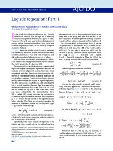
Outlier Detection in Logistic Regression: A Quest for Reliable Knowledge from Predictive Modeling and Classification Abdul Nurunnabi, Geoff West Department of Spatial Sciences, Curtin University, Perth, Australia

CRC for Spatial Information (CRCSI) [email protected] [email protected]

Objectives  Identification of multiple influential observations in logistic regression  Classification of outliers on a graphical plot  Investigating importance of outlier treatment for reliable knowledge discovery

Outlier (what, when and how?) An outlier is an observation that deviates so much from the other observations as to arouse suspicions that it was generated by a different mechanism. Hawkins (1980)

Causes of outliers: Outliers occur very frequently in real data, and often go unnoticed because much data is processed by computers without careful inspection and screening. They may appear because of human error such as keypunch errors, mechanical faults (such as transmission or recoding errors), changes in system behavior, exceptional events (natural disasters such as earthquakes and floods), instrument error, or simply through natural deviations in populations. Outliers’ effects: The presence of outliers in a dataset may cause the parameter estimation to be erroneous, misclassifying the outcomes and consequently creating problems when making inferences with the wrong model. Draws unreliable conclusions and decisions.

Outliers and Reliability Issues

The typical steps constituting the KDD process

Reliability issue and outlier interact with 5 questions [Fayyad et al. 1996; Dai et al. 2012] : i.

What are the major factors that can make the discovery process unreliable?

ii. How can we make sure that the discovered knowledge are reliable? iii. Under what conditions can a reliable discovery be assured? iv. What techniques are there that can improve the reliability of discovered knowledge? v. When can we trust that the discovered knowledge is reliable and reflects the real data?

Logistic Regression Logistic regression is useful for situation in which we want to predict the response (presence or absence) of a characteristic or outcome based on values of a set of predictor variables. It can be classified into three types based on categorical response variables: binary, ordinary and nominal.  A binary response has two categories with no natural order (for example, success-failure or yes-no).  An ordinal response has three or more categories with a natural ordering (e.g. none, mild, and severe).  A nominal response has three or more categories with no natural ordering (for example, blue, black, red, yellow; or sunny, rainy, and cloudy). In this presentation, we will cover only the binary logistic regression.

Logistic Regression and Outlier The customary model for LR is: E (Y | X ) = π ( X )

The log of [π (.)/(1-π (.))] can be defined as a linear function called logit (log odds) of X  π  g ( X ) = ln  = log(odds) = β0 + β1 X 1 +  + β p X p = Xβ 1− π 

e β0 + β1 X 1 ++ β p X p , 0 ≤ π ≤1 where π = β0 + β1 X 1 ++ β p X p 1+ e

The LR model can be re-written as: Y =π+ε where Y is a vector of binary (0, 1) response and ε is the error term:  1 − π with probability ε= with probability − π

π;

if

1 − π; if

y = 1, y = 0.

Outliers, linear and logistic (S-curve) models.

Types of Outliers Typically outliers in regression can be categorized into three classes: outliers, high leverage points and influential observations.  Deviation/change in X (explanatory) space, called leverage points  Deviation in Y (response variable) not in X, called vertical outliers  Deviation in both (X-Y) spaces. Influential observations are defined as points, which either Individually or together with several other observations, have a demonstrably larger impact on the calculated values of various estimates (coefficients, standard errors, t-values etc.). (Belsley et al. 1980) In logistic regression, outliers and influential observations may occur as misclassification between the binary (0, 1) responses. It may occur by meaningful deviation (we also see low leverage) in explanatory variables. (Nurunnabi et al. 2010)

Outlier Detection: Single-case Deletion Approach The ith residual can be defined in LR as:

εˆi = yi − πˆ i The projection (leverage) matrix is a diagonal matrix that gives the fitted values of the response variable as the projection onto the covariate space. It is defined as: where V is a diagonal matrix with H = V 1 / 2 X ( X T VX ) −1 X T V 1 / 2

The ith diagonal element of H defined as:

hii =

πˆ i (1 − πˆ i ) xiT ( X T VX ) −1 xi

diagonal elements vi

= πˆ i (1 − πˆ i )

hii > ck/n ( c = 2 or 3) values are generally identified as high leverage points. k=p+1.

The standardized Pearson residual for LR is defined as: rsi =

yi − πˆ i vi (1 − hii )

| rsi |≥ 3

are generally identified as outliers

DFFITS in LR defined as: DFFITSi =

yˆ i − yˆ i( −i )

vi( −i )

hii

DFFITS > 3√(k/n) are identified as influential cases

Modification for Group Deletion Approach The single-case deletion measures are naturally affected by the masking and swamping phenomena and fail to detect outliers in the presence of multiple outliers and/or influential cases. Masking occurs when an outlying subset goes undetected because of the presence of another, usually adjacent, subset. Swamping occurs when good observations are incorrectly identified as outliers because of the presence of another, usually remote subset of observations. The group deletion approach forms a clean subset of the data that is presumably free of outliers, and then test the outlyingness of the remaining points relative to the clean subset.

Outlier Detection: Group Deletion Approach These methods find a suspect group (D) of d outlying/unusual cases with the help of graphical methods, robust techniques such as LMS, RLS and/or appropriate diagnostics measures. The data in explanatory variables (X), response variable (Y) and the variancecovariance matrix V can be separated (deletion group D and the clean set R) as: 0 X  Y  V X =  R , Y =  R , V =  R  X D YD   0 VD 

Generalized Standardized Pearson Residual (GSPR) yi − πˆ i ( R )    vi ( R ) (1 − hii ( R ) ) rsi* =  yi − πˆ i ( R )   vi ( R ) (1 + hii ( R ) ) 

for i ∈ R, rsi* ≥ 3 are generally

for i ∈ D,

for i ∈ R, for i ∈ D.

(

(

i

)

( R)

)

εˆi ( R ) = yi − πˆ i ( R ) , vi ( R ) = πˆi ( R ) (1 − πˆ i ( R ) )

identified as outliers

hii ( R ) = πˆi ( R ) (1 − πˆi ( R ) ) xiT ( X RTVR X R ) −1 xi

Generalized Weight (GW)  hii ( R )   1 − hii ( R ) * hii =  h  ii ( R )  1 + hii ( R )

πˆ i ( R )

exp xi T βˆ( R ) = 1 + exp x T βˆ

hii* > median ( hii* ) + 3 × MAD ( hii* ) are identified as high leverage points

Identification of Multiple Influential Observations Mahalanobis Distance MDi = ( Z i − Z )T Σ −1 ( Z i − Z )

where Z is an m variate with mean Z and covariance matrix Σ . The proposed Influence Distance (ID): IDi =

(Gi − G(R ) )T Σ (−1R ) (Gi − G(R ) )

where G = [ rsi* hii* ] is the generalized residual-leverage matrix and G( R ) and Σ ( R ) are the mean and covariance matrix based on the R group (excluding the observations are identified as outliers by GSPR) .

Proposed Method Algorithm 1. (i)

Calculate rsi* and hii* using the group deletion approach

(ii)

Construct the matrix G = [ rsi*

(iii)

Calculate G( R ) and Σ ( R ) based on the R group after the

hii* ]

deletion of outlying cases (iv)

T Calculate IDi = (Gi − G(R ) ) Σ (−1R ) (Gi − G(R ) )

(v)

Find influential observations for which IDi > χ 22, 0.975 = 2.716

(vi)

To sketch the classification plot : (a) draw an scatter plot

rsi* versus hii* (b) draw cut-off lines at ±3 and median ( hii* ) + 3 × MAD ( hii* )

through the rsi* and hii* axes

respectively (c) draw an influence ellipse based on the ID values and the Chi-square cut-off value.

Classification plot.

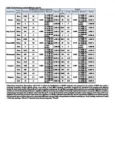
Experiment 1. Modified Brown Data Diagnostic Results for Modified Brown Data Modified Brown Data i L.N.I. A.P. i L.N.I. A.P. i L.N.I. A.P. i L.N.I. A.P. 1 0 48 15 0 47 29 0 50 43 1 81 2 0 56 16 0 49 30 0 40 44 1 76 3 0 50 17 0 50 31 0 55 45 1 70 4 0 52 18 0 78 32 0 59 46 1 78 5 0 50 19 0 83 33 1 48 47 1 70 6 0 49 20 0 98 34 1 51 48 1 67 7 0 46 21 0 52 35 1 49 49 1 82 0 75 36 0 48 50 1 67 8 0 62 22 9 1 56 23 1 99 37 0 63 51 1 72 10 0 55 24 0 187 38 0 102 52 1 89 11 0 62 25 (1)0 136 39 0 76 53 (1)0 126 12 0 71 26 1 82 40 0 95 54 0 200 13

0

65 27

0

40 41

0

66 55

14

1

67 28

0

50 42

1

84

0 220

i

|rsi| (3.00)

1 2 3 4 5 6 7 8 9 10 11 12 13 14 15 16 17 18 19 20 21 22 23 24 25 26 27 28

-0.740 -0.728 -0.737 -0.734 -0.737 -0.739 -0.743 -0.719 1.406 -0.729 -0.719 -0.707 -0.715 1.431 -0.742 -0.739 -0.737 -0.699 -0.693 -0.678 -0.734 -0.702 1.520 -0.634 -0.650 1.469 -0.753 -0.737

hii |DFFITSi| |rsi*| hii* IDi (0.073) (0.572) (3.00) (0.081) (2.716) 0.029 0.023 0.027 0.026 0.027 0.028 0.030 0.020 0.023 0.024 0.020 0.018 0.019 0.019 0.029 0.028 0.027 0.019 0.020 0.027 0.026 0.018 0.028 0.186 0.074 0.019 0.036 0.027

-0.124 -0.110 -0.120 -0.116 -0.120 -0.122 -0.128 -0.102 0.216 -0.111 -0.102 -0.095 -0.099 0.198 -0.126 -0.122 -0.120 -0.093 -0.094 -0.106 -0.116 -0.094 0.244 -0.275 -0.167 0.201 -0.141 -0.120

-0.520 -0.615 -0.543 -0.566 -0.543 -0.531 -0.499 -0.698 1.672 -0.602 -0.698 -0.849 -0.745 1.315 -0.510 -0.531 -0.543 -0.993 -1.114 -1.584 -0.566 -0.928 0.689 -9.979 0.274 0.964 -0.441 -0.543

0.040 0.029 0.037 0.034 0.037 0.038 0.043 0.024 0.029 0.030 0.024 0.026 0.023 0.023 0.042 0.038 0.037 0.038 0.052 0.114 0.034 0.032 0.118 0.051 0.126 0.049 0.052 0.037

0.578 0.906 0.655 0.739 0.655 0.615 0.515 1.104 1.696 0.866 1.104 1.165 1.159 1.428 0.545 0.615 0.655 1.063 1.101 2.624 0.739 1.108 2.706 9.995 2.837 1.003 0.459 0.655

i 29 30 31 32 33 34 35 36 37 38 39 40 41 42 43 44 45 46 47 48 49 50 51 52 53 54 55

|rsi| hii |DFFITSi| (3.00) (0.073) (0.572) -0.737 -0.753 -0.729 -0.723 1.391 1.396 1.393 -0.740 -0.718 -0.674 -0.701 -0.681 -0.714 1.475 1.466 1.453 1.438 1.458 1.438 1.431 1.469 1.431 1.443 1.489 -0.656 -0.634 -0.637

0.027 0.036 0.024 0.022 0.029 0.026 0.028 0.029 0.020 0.030 0.018 0.025 0.019 0.020 0.019 0.018 0.018 0.019 0.018 0.019 0.019 0.019 0.018 0.022 0.058 0.222 0.281

-0.120 -0.141 -0.111 -0.106 0.237 0.228 0.234 -0.124 -0.101 -0.111 -0.093 -0.103 -0.098 0.204 0.200 0.196 0.196 0.197 0.196 0.198 0.201 0.198 0.195 0.214 -0.148 -0.308 -0.366

hii* IDi |rsi*| (0.081 (3.00) (2.716) ) -0.543 0.037 0.655 -0.441 0.052 0.459 -0.602 0.030 0.866 -0.655 0.026 1.017 1.998 0.040 1.994 1.869 0.035 1.863 1.954 0.038 1.948 -0.520 0.040 0.578 -0.714 0.023 1.126 -1.740 0.131 3.173 -0.949 0.034 1.091 -1.476 0.101 2.215 -0.761 0.023 1.170 0.926 0.056 1.054 0.983 0.046 0.999 1.089 0.034 1.113 1.234 0.025 1.335 1.045 0.038 1.048 1.234 0.025 1.335 1.315 0.023 1.428 0.964 0.049 1.003 1.315 0.023 1.428 1.183 0.027 1.264 0.839 0.075 1.420 0.339 0.132 3.061 -13.311 0.037 13.426 -20.662 0.021 20.914

Experiment 1. Modified Brown Data

Modified Brown data (a) scatter plot; L.N.I. versus A.P. (b) index plot of standardized Pearson residual (c) index plot of leverage values (d) index plot of DFFITS (e) index plot of GSPR (f) index plot of GW (g) index plot of ID (h) classification plot

Experiment 2. Modified Finney Data Diagnostic Results for Modified Finney Data

Modified Finney Data i Y Vol. Rate i Y Vol. Rate i Y Vol. 1 1 3.70 0.825 14 1 1.40 2.330 27 1 1.80 2 1 3.50 1.090 15 1 0.75 3.750 28 0 0.95 3 1 1.25 2.500 16 1 2.30 1.640 29 1 1.90 4 1 0.75 1.500 17 1 3.20 1.600 30 0 1.60 5 1 0.80 3.200 18 1 0.85 1.415 31 1 2.70 6 1 0.70 3.500 19 0 1.70 1.060 32 0 2.35 7 0 0.60 0.750 20 1 1.80 1.800 33 0 1.10 8 0 1.10 1.700 21 0 0.40 2.000 34 1 1.10 9 0 0.90 0.750 22 0 0.95 1.360 35 1 1.20 10 (0)1 0.90 0.450 23 0 1.35 1.350 36 1 0.80 11 (0)1 0.80 0.570 24 0 1.50 1.360 37 0 0.95 12 0 0.55 2.750 25 1 1.60 1.780 38 0 0.75 13 0 0.60 3.000 26 0 0.60 1.500 39 1 1.30

Rate 1.500 1.900 0.950 0.400 0.750 0.030 1.830 2.200 2.000 3.330 1.900 1.900 1.625

i 1 2 3 4 5 6 7 8 9 10 11 12 13 14 15 16 17 18 19 20

hii |DFFITSi| |rsi*| hii* IDi |rsi| hii |DFFITSi| |rsi| i (3.00) (0.154) (0.832) (3.00) (0.044) (2.716) (3.00) (0.154) (0.832) 0.1491 0.072 -0.127 0.000 0.00000 0.532 21 -0.6157 0.100 -0.201 0.1543 0.068 -0.112 0.000 0.00000 0.532 22 -0.7032 0.061 -0.175 0.5799 0.061 0.148 0.035 0.01708 0.444 23 -1.0176 0.045 -0.194 1.6914 0.071 0.353 587.164 0.00013 965.085 24 -1.1836 0.048 -0.210 0.6074 0.118 0.209 0.041 0.02304 0.417 25 0.6301 0.052 0.134 0.5683 0.149 0.215 0.020 0.00763 0.489 26 -0.5520 0.084 -0.166 -0.3570 0.093 -0.099 0.000 0.00000 0.532 27 0.6174 0.067 0.143 -0.9807 0.039 -0.190 -0.110 0.06880 0.357 28 -0.9577 0.044 -0.201 -0.4759 0.094 -0.150 0.000 0.00000 0.532 29 0.7854 0.096 0.222 2.7516 0.102 0.790 44522.925 0.00000 73194.797 30 -0.7693 0.128 -0.244 2.8168 0.098 0.774 56039.735 0.00000 92128.254 31 0.4223 0.160 0.184 -1.1087 0.110 -0.359 -0.276 0.27368 0.572 32 -1.3568 0.288 -0.444 -1.3554 0.124 -0.459 -1.997 0.90055 3.504 33 -1.0578 0.037 -0.200 0.5540 0.058 0.134 0.023 0.00941 0.480 34 0.7921 0.045 0.171 0.4682 0.151 0.171 0.003 0.00043 0.528 35 0.8071 0.039 0.161 0.3559 0.088 0.096 0.000 0.00001 0.532 36 0.5649 0.126 0.201 0.1516 0.057 -0.127 0.000 0.00000 0.532 37 -0.9577 0.044 -0.201 1.6115 0.066 0.335 386.514 0.00026 635.219 38 -0.7972 0.061 -0.198 1.072 39 0.9132 0.037 0.173 -1.2160 0.073 -0.243 -0.718 0.21561 0.5176 0.066 0.122 0.012 0.00351 0.511

|rsi*| (3.00) -0.001 -0.005 -0.151 -0.615 0.079 0.000 0.061 -0.086 0.576 -0.008 0.001 -1.144 -0.229 0.731 0.870 0.020 -0.086 -0.015 2.658

hii* IDi (0.044) (2.716) 0.00007 0.533 0.00068 0.532 0.09264 0.331 0.17485 0.937 0.05443 0.288 0.00001 0.533 0.03996 0.344 0.05323 0.389 0.42628 1.829 0.00156 0.531 0.00009 0.531 1.28008 4.314 0.14620 0.342 0.30392 1.639 0.24012 1.678 0.00801 0.488 0.05323 0.389 0.00438 0.524 0.18395 4.477

Experiment 2. Modified Finney Data

Modified Finney data (a) character plot; rate versus volume with the response values (1, 0) (b) index plot of standardized Pearson residual (c) index plot of leverage values (d) index plot of DFFITS (e) index plot of GSPR (f) index plot of GW (g) index plot of log(ID) (h) classification plot.

Reliability Checking: Models Parameters Estimation and Test Modified Brown Data LR model fit and significance test Results for all observations Parameter estimation Odds 95% Conf. Int. Predictor Coef. S. E. Z P Ratio Lower Upper Constant -0.463 0.674 -0.69 0.492 A.P. -0.003 0.008 -0.42 0.677 1.00 0.98 1.01 Test Test that all slopes are zero: G = 0.183, df = 1, P-Value = 0.669 Goodness -of-fit test df p Χ2 Pearson 42.144 34 0.159 Deviance 53.407 34 0.018 Hosmer-Lemeshow (H-L) 23.059 8 0.003 Model Summery Log-Likelihood (LL) -2 LL Cox & Snell R2 Nagelkerke R2 -34.681 69.363 0.003 0.005

Results without outliers Parameter estimation 95% Conf. Int. Odds Coef. S. E. Z P Ratio Lower Upper -4.134 1.486 -2.78 0.005 0.055 0.022 2.51 0.012 1.06 1.01 1.10 Test Test that all slopes are zero: G = 7.31, df = 1, P-Value = 0.007 Goodness -of-fit test χ2 Df p Pearson 33.295 28 0.225 Deviance 41.167 28 0.052 Hosmer-Lemeshow (H-L) 6.044 8 0.642 Model Summery Log-Likelihood (LL) -2 LL Cox & Snell R2 Nagelkerke R2 - 28.562 57.123 0.139 0.190

Predicted probabilities versus A.P.

Performance Evaluation: Classification

Classification results with outliers and without outliers All observations Predicted Actual Status status Absence Presence Total (0) (1) Absence 32 23 55 (0) (58.18%) (41.82 %) (100%) Presence 0 0 0 (1) (0%) (0%) (0%) 23 32 Total 55 (58.18%) (41.82 %) Correct 58.18% classif.

Without outliers Actual status Absence Presence Total (0) (1) 25 10 35 (45.45%) (18.18%) (63.64%) 7 13 20 (12.73%) (23.64%) (36.36%) 32 23 55 (58.18%) (41.82%) 69.09%

Mosaic plot (a) classification with outliers (b) classification without outliers

Performance Evaluation: Predictive Ability

ROC Curves results

All observations Without outliers

Area

S. E.

0.219 0.781

0.064 0.064

Sig. (p) 0.000 0.000

Asymptotic 95% Conf. Int. Lower Bound Upper Bound 0.094 0.345 0.655 0.906

ROC curve (a) data with outliers (b) data without outliers

Conclusions This paper proposes a diagnostic measure for identifying multiple influential observations in logistic regression. It introduces a classification graph to classify outliers, high leverage points and influential observations in the same plot at one time. Diagnostic results show that the proposed measure efficiently identifies multiple influential cases, and the graph is helpful for visualizing outlier categories. Results show that without careful outlier investigation, it may not be possible to get reliable knowledge using logistic regression for predictive modeling and classification.

Conclusions The outlier investigation in logistic regression is highly related to the issues raised for reliable knowledge discovery. (i) Outlier detection is one of the major factors that affect the reliability of the discovery process. (ii) The conditions for reliable knowledge discovery can be improved by parameter estimation and testing the significance of the estimates. (iii) Proper outlier diagnostics and treatment (deletion or correction of the outlying observations) can improve the reliability of discovered knowledge. (iv) We can trust the discovered knowledge is reliable and reflects the real data if the test results meet the required statistical significance level. Therefore outlier detection and proper treatment is vital for obtaining reliable knowledge, and should be considered as a data preprocessing step in knowledge discovery in databases (KDD). The proposed diagnostic method is introduced for the binomial response variable in logistic regression. Future research will investigate the diagnostic method for (i) multinomial response variables, and (ii) large and high dimensional data as higher dimensional data presents extra problems that need to be addressed.

Question ?