Detection and identification of anomalies in wireless mesh networks using Principal Component Analysis (PCA) Zainab R. Zaidi, Sara Hakami, Bjorn Landfeldt, and Tim Moors August 06, 2008 Regular paper submission to: World Scientific Journal of Interconnection Networks (JOIN) ∗
Corresponding Author: Zainab Zaidi Author Contact Information:
Zainab R. Zaidi Network Systems NICTA Locked Bag 9013 Alexandria, NSW 1435 Australia tel: (612) 8374 5235 fax: (612) 8374 5531
[email protected]
Sara Hakami School of EE&T University of NSW Sydney, NSW 2052, Australia also at NICTA
[email protected]
Bjorn Landfeldt School of IT University of Sydney Sydney, NSW 2006 Australia also at NICTA tel: (612) 9351 8962 fax: (612) 9351 3838
[email protected]
Tim Moors School of EE&T University of NSW Sydney, NSW 2052 Australia also at NICTA fax: (612) 9385 5993
[email protected]
1
Abstract Anomaly detection is becoming a powerful and necessary component as wireless networks gain popularity. In this paper, we evaluate the efficacy of PCA based anomaly detection for wireless mesh networks (WMN). PCA based method [1] was originally developed for wired networks. Our experiments show that it is possible to detect different types of anomalies, such as Denial-of-service (DoS) attack, port scan attack [1], etc., in an interference prone wireless environment. However, the PCA based method is found to be very sensitive to small changes in flows causing non-negligible number of false alarms. This problem prompted us to develop an anomaly identification scheme which automatically identifies the flow(s) causing the detected anomaly and their contributions in terms of number of packets. Our results show that the identification scheme is able to differentiate false alarms from real anomalies and pinpoint the culprit(s) in case of a real fault or threat. Moreover, we also found that the threshold value used in [1] for distinguishing normal and abnormal traffic conditions is based on assumption of normally distributed traffic which is not accurate for current network traffic which is mostly self-similar in nature. Adjusting the threshold also reduced the number of false alarms considerably. The experiments were performed over an 8 node mesh testbed deployed in a suburban area, under different realistic traffic scenarios. Our identification scheme facilitates the use of PCA based method for real-time anomaly detection in wireless networks as it can filter the false alarms locally at the monitoring nodes without excessive computational overhead.
I. Introduction With growing popularity of wireless mesh networks, it is becoming critically important to work towards providing similar quality-of-service to the users as they are accustomed to in networks with wired infrastructure. The cost-effectiveness of wireless mesh solutions for backhaul networks is the major factor in attracting a lot of interest from various industrial and academic entities. There are, however, only pilot and experimental deployments of wireless mesh networks at the moment, e.g., MIT Roofnet [2], Wray village [3], etc. Comparing with the wired networks, there is also not much experience with real incidents and security issues. But it is not difficult to envision the additional vulnerabilities associated with WMN which should be taken care of before any major deployment. The most interesting difference, between a wired and a wireless infrastructure network, lies in the fact that links are relatively unreliable, dynamic, and resource constraint in nature.
2
Moreover, the unprotected locations of wireless routers expose them to malicious intrusions, such as, jamming, Denial-of-Service (DoS) attack, and environmental hazards, e.g., thunder storms, etc. [4]. As a consequence of faults (natural and man-made), wireless mesh networks might perform inefficiently. Malfunctions, such as node failures, DoS, etc., can have a more severe impact in wireless networks than wired networks due to limited and shared resources. Since WMN is a recent development, not many schemes are developed for fault management. A brief overview of fault detection/management techniques is done in Section II and their respective merits and demerits are pointed out. The focus of our research is towards the idea of detecting faults through passive monitoring only, as additional overhead might be detrimental to network performance [5]. Our recent work [6] utilizes the information in packet headers and control messages to detect routing misbehavior. In this paper, we look at the traffic volume, in terms of number of packets and flows, in order to detect the anomalies affecting it, such as, DoS, port scan, jamming, etc. Anomaly detection method presented in [1] is our starting point as it is already shown to be very effective in detecting traffic anomalies, e.g., DoS, port scan, etc., in wired networks. In this paper, we evaluate the effectiveness of anomaly detection method presented in [1] for wireless networks through an experimental study. Since wireless links have higher interference and variability than wired links it was not known if the method would be able to detect anomalies in noisy environments while keeping the false alarm rate at a reasonable level. The method of [1] is found to be very sensitive to small changes in flows causing non-negligible number of false alarms. Prompted by the high false alarm, we have also enhanced the Principal Component Analysis (PCA) based anomaly detection method of [1] to automatically identify the nodes causing the anomalies and estimate their contribution in terms of number of packets and flows. Moreover, we also found that the threshold value used in [1] for distinguishing normal and abnormal traffic conditions is based on assumption of normally distributed traffic which is not accurate for current network traffic which is mostly self-similar in nature. Our alternative approach of estimating the threshold also reduced the number of false alarms considerably.
3
Integrated with our identification scheme and threshold adjustment, PCA based method of anomaly detection is a promising solution for real-time anomaly detection in WMN. Principal Component Analysis (PCA) maps the data into orthogonal axes or principal components (PCs) which are sorted according to the variation of data they capture. The variation is represented by the eigenvalues associated with PCs. PCA has been effectively used to detect various types of anomalies in wired networks [7], [1], [8]. PCA is used to reduce the dimensions of the space spanned by network traffic by considering the significant PCs only. It is shown that most of the traffic variations is captured by few PCs in [1] and the fact is also confirmed by our experiments. Any threshold based technique to detect significant deviation from normal trend is much easier to implement over the reduced space rather than over the aggregated traffic. Lakhina et al. use Hotelling’s t2 statistics to effectively detect the data points deviating far from the mean traffic conditions [7]. Our experimental results show that PCA with t2 statistics is able to detect the anomalies in a rich mix of network traffic over wireless mesh networks. Although, the method is found to be very sensitive to the perturbations usual for self-similar traffic and results in non-trivial number of false alarms. Major cause of false alarms is the inaccurate assumption, used in calculations of t2 threshold, of considering normally distributed network traffic. Self-similar traffic distribution is relatively heavy-tailed when compared with normal distribution with higher likelihood of false alarms for same threshold. We have tried different approaches for threshold calculation to reduce the false alarm rate. Moreover, the sensitivity of PCA using t2 statistics to small traffic perturbations prompted us to investigate automatic identification of the source of the detected anomaly and its contribution in terms of number of packets or flows. If this contribution is small enough, our scheme disregards the detection and if the contribution is significant, it reports an anomaly. Our identification method maps the principal components back into the measurement space to pick the data corresponding to the anomalous principal components at specific time bins. The automatic identification is very useful in reducing the number of false alarms and in-
4
creasing the efficiency of PCA based method in anomaly detection. In our experiments, we are able to distinguish false alarms from real anomalies. Moreover, the identification method correctly points out the traffic flows responsible for real faults as shown in our experimental results. The rest of the paper is organized as follows: Section II contains a summary of literature survey, Section III briefly discusses the principal component method presented in [7], [1], [8], Section IV develops the method for automatic identification of causes, Section V presents details about our wireless mesh testbed, experiments and results, and finally Section VI concludes the paper. II. Related Work Since WMN is a recent development, not many schemes are developed for fault management. A comprehensive survey of fault management techniques in wireless multihop networks is done in [9]. On the other hand, a huge volume of mature research is present in anomaly/fault detection in wired networks [1]. In wireless multihop networks, largely for ad hoc and sensor networking scenarios, research is limited to either threshold-based techniques where loss of a certain number of ACKs or periodic updates trigger route recovery [9], or intrusion detection techniques, where incoming and outgoing links of each node are monitored locally for abnormal behavior, such as, artificial immune system (AIS) [10] and watchdog [11]. These techniques either require all nodes to monitor their neighbors, causing trust issues, or they require a high density of robust monitors which makes them very expensive. Recently, work is being done to establish the requirements of a fault management system for WMN [12], [13] and to study the effects of monitoring over network performance [5]. Moreover, specific security issues and challenges of WMN scenario are outlined in [4], [14]. Qiu et al. developed the first, according to our knowledge, fault detection scheme for WMN [15]. They trained a simulator by traffic traces of WMN and used it for distinguishing normal and abnormal traffic patterns. This scheme, though able to detection variety of
5
faults, heavily depends on the accuracy and flexibility of simulator and the quality of traffic traces. Moreover, in order to adapt to a dynamic system, the simulator would need frequent training periods increasing the cost of the scheme. Also, a simulator driven approach is not suitable for real-time fault detection. In wired network research, statistical methods are widely used for anomaly detection including PCA-based method [1]. These methods used statistical distributions (KolmogorovSimrnov test) [16], wavelets [17], and frequency distributions [18]. Kolmogorov-Smirnov test [16] is able to detect the anomalous traffic but it is not able to identify the cause of the anomaly. Wavelets can detect congestion by comparing the energy distributions over various wavelet components in normal and anomalous situations but it cannot be used in real-time as it is computationally intensive and requires complete data sets for processing. PCA-based method is, however, computationally light weight and can be used to run online. There are other techniques proposed in [19] and [20] very similar to the PCA-based method where the difference in normal and anomalous traffic is quantified and compared against certain thresholds. III. PCA in anomaly detection As summarized in [8], PCA is a coordinate transformation method that maps the measured data onto a new set of axes called the principal axes or components. Each principal component has the property that it points in the direction of maximum variance remaining in the data, given the variance already accounted for the preceding components. This way, the first principal component is directed towards the maximum variance of the original data. The second principal component is orthogonal to the first and represents the maximum residual variance among the remaining directions. The number of packets transmitted during each interval of the observation window, sorted according to OD (Origin-Destination) flow, is stored as one of the columns of a matrix called X of size p × l, assuming that there are l OD flows available for p successive intervals. Thus,
6
each column i denotes the time-series of the i-th OD flow and each row j represents an instance of all the OD flows at interval j. Each principal component vi is the i-th eigenvector computed from the spectral decomposition of X T X, where X = X − X¯ and X¯ is the time average of X . This normalization ensures that PCs capture the common temporal trends in traffic and are not skewed by the differences in mean OD flow rates. X T Xvi = λi vi ,
i = 1, · · · , l
(1)
where λi is the eigenvalue corresponding to vi . Furthermore, because X T X is symmetric positive definite, its eigenvectors are orthogonal and the corresponding eigenvalues are nonnegative real. By convention, the eigenvectors have unit norm and the eigenvalues are arranged from large to small, so that λ1 ≥ λ2 ≥ · · · λl . Considering the data mapped onto the principal components, it is clear that the contribution of principal axis i as a function of time is given by Xvi [8]. This vector can be √ normalized to unit length by dividing by σi = λi . Thus, for each principal axis i, ui =
Xvi , i = 1, · · · , l. σi
(2)
The ui ’s are vectors of size p that are orthogonal by construction. The above equation shows that all the OD flows, when weighted by vi , produce one dimension of the transformed data. Thus vector ui captures the temporal variation common to all flows along principal axis i. Since the principal axes are in order of contribution to the overall variance, u1 captures the strongest temporal trend common to all OD flows, u2 captures the next strongest, and so on. Because the set of {ui }li=1 capture the time-varying trends common to the OD flows, they are referred as the eigenflows of X [8]. A. The Effective Subspace The elements of {σi }li=1 are called the singular values [8]. Note that each singular value is the square root of the corresponding eigenvalue, which in turn is the variance attributable
7
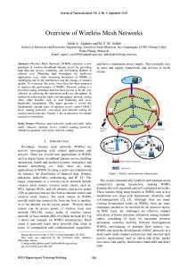
Fig. 1. Scree plot for traffic captured at node mesh06 in a day-long experiment.
to the respective principal component: ||Xvi || = viT X T Xvi = λviT vi = λi ,
(3)
where the second equality holds from equation (1) and the last equality follows from the fact that vi has unit norm. Thus, the singular values are useful for gauging the potential for reduced dimensionality in the data, often simply through their visual examination in a scree-plot [8]. Specifically, finding that only r singular values are non-negligible, implies that X effectively resides on an r-dimensional subspace of Rl . In this case, the original X can be approximated as: 0
X ≈
r X
σi ui viT .
(4)
i=1
For example, in the traffic captured at node mesh06 in one of our day-long experiments (cf. Section V-B), the scree-plot clearly shows an elbow above principal component 2 in Fig. 1. Therefore the value of r can be as small as 2, and in fact the first two PCs might explain up to 99.9% of the total variability of the specific data set. The rest of the PCs define the
8
˜ i.e., residual subspace X, ˜ X = X 0 + X.
(5)
In [1], the effective subspace X 0 is called normal subspace and the main idea is to separate the network traffic into normal and abnormal subspaces where abnormal subspace is ˜ It is shown in [1] that different anomalies become prominently visible in equivalent to X. the abnormal subspace using residual analysis and anomaly detection with subspace division works better than any threshold based technique over aggregated traffic volume. Squared prediction error (SPE) of eigenflows in abnormal subspace is suggested as a method to detect anomalies [1]: ˜ 2 > δs SPEj = ||X|| j
(6)
where SP Ej is the SPE at jth interval, δs is the threshold for the SPE, and ˜= X
l X
σi ui viT
(7)
i=r+1
The selection of δs is discussed in detail in [1]. Although, in our experiments, we realized that since most of the network traffic is effectively characterized by X 0 , the anomalies are ˜ As a result the performance of SPE is very poor as also contained in X 0 rather than X. compared to t2 statistics and results in significant number of missed detections and false alarms. Other alternative methods for decomposition of principal components are also discussed in [1], such as the threshold-based separation method. The threshold-based technique examines each eigenflow and if found to exceed a threshold (e.g., 3 times standard deviation away from the data mean), that eigenflow and all subsequent flows are assigned to the residual subspace ˜ X.
9
B. Hotellings’ t2 Statistics Hotelling’s t2 is a statistical measure of the multivariate distance of each observation from the center of the data set (for eigenflows, the center is zero by construction [7]). This represents an analytical way to identify the most extreme points in the data by calculating the sum of squares at each interval j of the eigenflows in the normal subspace, as follows: t2j
=
r X
u2ij ,
j = 1, · · · , p.
(8)
i=1
A peak in the t2 graph exceeding the threshold δt as defined in [7] is considered an anomaly. δt =
r(p − 1) Fr,p−r,α , p−r
(9)
where Fr,p−r,α is the value of F distribution with r and p − r degrees of freedom at the 1 − α confidence level. The threshold for t2 in (9) is accurate if the underlying data, i.e., X is normally distributed. In our case, network traffic is typically self-similar which would result in a heavier tailed distribution. Threshold defined in (9) may result in high rate of false alarms as shown in [21]. We propose a new threshold according to the Chebyshev inequality which states that P(|Y − µy | ≥ kσy ) ≤
1 , k2
where Y could be any data set with mean µy and standard deviation σy and k is a constant. A threshold of δt = 4σt2 ,
(10)
where σt2 is the standard deviation of t2 vector calculated from (8), will ensure that 94% of the data will reside under the threshold. A threshold of δt = 7σt2 could be used for 98% confidence bound. Since Chebyshev inequality is a weaker upper-bound, the chances of missed detection will increase with higher threshold. A positive aspect of this threshold is its distribution independence. However, if data distribution is closer to normal, (9) is a better threshold.
10
C. Other ways of constructing X In addition to analyzing packet counts, anomalies can also be detected by analyzing byte and flow counts. For example, a port scan attack might not result in change in number of packets for OD flows but it certainly increases the number of flows in the network, where flows are sorted according to the port numbers. This change would result in a peak in t2 statistics which are derived from X containing the flow counts in the network [7]. Similarly a bandwidth measurement experiment [7] could be easier to detect when X is constructed using number of bytes per OD flow instead of number of packets. Incorporation of multiple representation of network traffic is a powerful attribute of the PCA based anomaly detection method which enables better detection capability as some anomalies might not be visible in one type of representation but become prominent in another. IV. Automatic identification of anomalies Once it is detected that the data contains some anomaly, it is vital to know: who caused it and what is the impact of the anomaly over the network traffic. Although, initially we started working in this direction in order to find a way to reduce the effects of false alarms, as a consequence of (9), but we realized that our identification scheme is a powerful extension in the PCA-based scheme. Our identification scheme can identify the OD flow or flows causing peaks in t2 and their contribution in terms of number of packets or flows. Our scheme helps eliminate the false alarms due to traffic perturbation besides providing an efficient way of identifying the anomalous OD flows and even help classify the type of specific anomaly in some cases. The principle behind our identification scheme is the reverse mapping of PCs into the measurement space. Once t2 detects an anomaly in a particular time bin, all significant contributing eigenflows and associated PCs are then mapped back to the measurement space or OD flows to identify the flow(s) causing the anomaly and also the number of packets
11
t2 = u1 = u2 =
u1 =
u3 =
u4 =
= Xv1=
σ
u4 =
= Xv4=
1
σ
4
Fig. 2. Reverse mapping of anomalous time bin in t2 vector in the measurement space.
introduced in the network by the anomalous flow(s). Figure 2 shows an illustration of the identification scheme when an anomaly is found in a time bin of t2 vector. The steps of the scheme are as follows: 1. When the value of t2 exceeds the threshold at interval J, pick all uiJ , used to calculate t2 . If the number of contributing eigenflows uiJ is large, very small contributors can be neglected at this stage. As shown in Fig. 2, u2 and u3 have small contributions, shown by green and rust color, while u1 and u4 have excessive contributions represented by red color. 2. For ukJ found in the above step, calculate the contribution Ci by each OD flow i in this peak as follows, Ci =
X
XJi vik
(11)
k
3. Significant Ci are the contributions in number of packets from the OD flows which are the most probable causes for the peak in t2 . For example, OD 01 and OD 10 are found to have significant contribution in the illustration of Fig. 2.
12
According to our experiments, this method is very effective in identifying anomalies which generate traffic, such as, DoS or port scan. However, anomalies such as node outages cannot be found using the above method as this method always looks for flows with larger packet count. An alternative way to identify the flows contributing in the peaks of t2 is through the decomposition of (8) using (2) and (4) as follows: " # r X X X X (v ) (v ) i k i n ck = Xjk Xjn t2j = , 2 σ i n i=1 k k
(12)
where (vi )k is the k th element of eigenvector vi , Xjk is the value of OD flow k at j th time bin, and ck is the contribution of k th OD flow. The OD flow k with the largest ck is the major contributor in the peak of t2 . Xjk is the packet contribution of k th OD flow if ck is found to be exceeding a percentage contribution threshold of Tc . In our experiments an arbitrary value for Tc is taken as 10. Since X is the normalized traffic vector, Xjk could be positive or negative. A negative value for Xjk shows the absence of packets with respect to the mean flow rate, which could happen in node outage scenario, and a positive value indicates the excess packets, such as, in DoS attack. According to our experiments, this method is very effective in identifying different anomalies, such as, DoS, port scan, and node outages. V. Experiments and results We used NICTA’s outdoor mesh network testbed for our experiments. The testbed has 7 nodes deployed at traffic intersections and one gateway mesh node inside the School of IT at University of Sydney. The Layout of the testbed with all the wireless links, is shown in Fig. 3. The testbed operates as an ad hoc LAN with no direct access to the outside world apart from a fixed link to the gateway node. Each node is equipped with three wireless interfaces: 2 WiFi (unlicensed bands) and 1 UnwiredTM (licensed band). UnwiredTM is the wireless broadband provider in Sydney at 3.5GHz. Unwired radios are used for control purposes in our testbed and are shown as curly arrows in Fig. 3. WiFi links exist between every two adjacent nodes and operate at channel 9 of the 2.4GHz band (802.11g), shown as thick lines
13
Fig. 3. Layout of NICTA’s outdoor testbed in Sydney.
in Fig. 3. Some nodes have extra WiFi links which operate at either 2.4GHz channel 1 (between mesh02 and mesh03), or 900MHz channel 4 (between mesh01-mesh05 and mesh04mesh07). WiFi links use omni-directional antennas. More details about the testbed can be found in [22]. The major purpose of NICTA’s wireless mesh testbed is to explore the technical feasibility and issues for a city-wide network used for control and monitoring applications such as, traffic signal control. Such a network requires high reliability although the typical traffic consists of packets with only a few bytes and bandwidth requirements are not as stringent as in a public access network. Based on this, our initial experiments used low volume data with small packets sizes. We used ICMP ping packets to simulate the situation of a control network. In subsequent experiments we used a traffic generator to provide a rich mix of flows and more diverse scenarios for experiments.
14
TABLE I Experiments with ping packets only using (9).
Normal traffic
Anomaly
Wireless type
Anomaly
False alarms
OD (ping interval(s), start bin)
Nodes (type, start bin)
1
01 (4, 1), 21 (10, 1), 51 (30, 30)
4 to 1 (ping flood, 88)
WiFi
yes
0
2
01 (4, 1), 21 (10, 1), 51 (30, 30)
3 to 1 (ping flood, 83-84)
UnwiredTM
yes
0
3
10 (4, 1), 12 (10, 1), 15 (30, 1)
2 (node failure, 106-109)
WiFi
yes
1
detected?
120
100
t2
80 based on Chebyshev inequality
60
40
20
based on F−distribution
0 0
20
40
60
80
100
120
Time bins Fig. 4. t2 statistics for experiment 1.
A. Experiments with low traffic Table I summarizes the initial ping based experiments. The column for normal traffic in Table I shows the flows in the form of “OD, (interval between successive pings in seconds, start time bin)”, where OD denotes origin and destination and 1 start bin refers that the experiment is started in the first time bin. Each time bin is 1 minute long. Note that in OD description, 1 refers to mesh01, 2 refers to mesh02, and so forth. All experiments ran over 2 hours and traffic data was collected from mesh01. Experiment 2 used UnwiredTM links where the rest of the experiments used 802.11 b/g links.
15
Fig. 4 shows t2 values for experiment 1. The horizontal dashed line is the t2 threshold calculated using (9) for 95% confidence interval. Note that (9) works fine for ping traffic as there is no issue of heavy-tailed self-similar distributed traffic. The dotted line shows the alternative threshold, given in (10), based on Chebyshev’s inequality. The alternative threshold of (10) is a loose upper-bound as shown in Fig. 4. The peak at 88th time bin refers to the ping flood. The anomaly identification scheme yields that approximately 639 additional packets, with respect to the mean flow rate, are being transmitted between nodes mesh01 and mesh04 in both ways. Since mesh01 is echoing back ping packets from mesh04, it is difficult to ascertain the identity of attacker in this case and further investigation is needed. The value of r for this experiment is 1. A similar experiment was repeated over UnwiredTM links and we observed symmetrical results. In experiment 2, only one PC is significant enough and is used for t2 calculations. Our identification scheme counted an aggregated number of 1594 excess packets for the ping flood detected at time bins of 83 and 84 between mesh01 and mesh03. We identified approximately 919 excess packets transmitted from mesh03 to mesh01, and unlike experiment 1 where both directions contributed equal number of packets, it shows that mesh03 is highly probable cause of the anomaly instead of mesh01. In experiment 1, the attacker could be either of the nodes. Fig. 5 shows the t2 statistics for experiment 3. In this case, 2 PCs were found significant and were used in the calculations of t2 . The node failure is detected at time bins 106-109, using the threshold given in (9), as shown in Fig. 5. In this case, the alternative threshold of (10) missed the anomaly as it is a loose upper-bound. For the detected anomaly at 106-109, our identification scheme shows the deficiency of approximately 6 packets in flows between mesh01 and mesh02, in both directions, when compared against the mean flow rates. The negative contribution values from the identification scheme serve as indicators for link or node outages. The second peak in Fig. 5 is identified as a false alarm. It was actually an attempt to establish ssh connection from a remote computer to mesh01 through the gateway,
16 120
100
t2
80 based on Chebyshev inequality
60
40
20 based on F−distribution 0 0
20
40
60
80
100
120
250
300
Time bins Fig. 5. t2 statistics for experiment 3. 80 70 60
t2
50 40 30 20
based on Chebyshev inequality based on F−distribution
10 0 0
50
100
150
200
Time bins Fig. 6. t2 statistics (flow count) for experiment 1 using traffic generator.
i.e., mesh00. All together 75 excess packets are counted for the false alarm peak due to ssh attempt. B. Experiments with traffic generator In order to create more interesting scenarios for experimentation, we used a traffic generator [23] which generates self-similar traffic flows according to an on-off model. Based on studies in [24], this traffic generator provided us with realistic IP traffic typical for a wireless
17
TABLE II Experiments with traffic generator.
1
Normal traffic
Anomaly
Anomaly
False alarms
False alarms
OD (a1 , a2 , a3 , a4 , a5 )
Nodes (type, start bin)
detected?
using (9)
using (10)
65 (5, 50, 1, 0.9, 2500.0),
6 to 5 (port scan, 221)
yes
0
0
5 (link outage, 234)
yes
0
0
15 (1, 1, 1, 0.9, 2500.0),
0 to 2 (ping flood, 594),
yes
20
0
13 (1, 2, 1, 0.9, 2500.0)
0 to all (node scan, 605-606),
64 (50, 5, 1, 0.9, 2500.0) 2
65 (5, 50, 1, 0.9, 2500.0), 64 (50, 5, 1, 0.9, 2500.0)
3
0 to 1 (UDP DOS, 920-922), 0 to 5 (port scan, 1235), 2 to 3 (port scan, 1211-1228), 0 to 1 and 2 (port scan, 940-941)
LAN. The following parameters are tunable for the traffic generator: 1. a1 = session arrival rate (no. of sessions/sec) 2. a2 = in-session packet arrival rate (no. of packets/sec for each session) 3. a3 = session duration parameter (sec) 4. a4 = Hurst parameter 5. a5 = service time distribution (no. of packets/sec) Table II summarizes three 24 hour long experiments. In experiment 1 and 2 two classes of traffic are generated from the mesh01 for mesh05 and mesh04. The parenthesis in second column contains the parameter settings for the traffic generator for each class. Data was collected at mesh05. Experiments 1 and 2 use 5 minute time bins. The threshold for t2 (9) is calculated for 95% confidence interval for all experiments. The alternative threshold is calculated using (10). The fourth column of Table II shows the detection results using both thresholds. We introduced single anomaly of port scan in experiment 1 and experiment 2
18 15
10
t2
based on Chebyshev inequality
based on F−distribution
5
0 0
50
100
150
200
250
300
Time bins Fig. 7. t2 statistics (flow count) for experiment 2 using traffic generator.
contains a natural link outage at node 5 as shown in Table II. Fig. 6 shows the t2 statistics for experiment 1 when data matrix X contains the flow count for each time bin. Port scan clearly results in a sharp peak in Fig. 6 at 221th time bin. The anomaly is not visible in packet and byte count analysis. The identification result shows approximately 18 excess flows at 221th time bin when compared against the mean number of flows in the experiment, although, flow count analysis is not able to pinpoint the cause of the anomaly. We repeated the analysis with flows counts sorted according to the sources and were able to identify mesh06 with approximately 8 additional flows. Fig. 7 shows the t2 statistics for experiment 2 when the traffic matrix contains flow count for each time bin. Fig. 7 shows the detection of link outage at 234th time bin as identification scheme yields deficiency of approximately 4 flows with respect to the mean flow count. When flows are sorted according to the sources, we are able to identify mesh05 with deficiency of 1 flow. In this experiment, packet and byte count analysis do not yield detection of link outage. Experiment 3 uses mesh01 as source and mesh03 and mesh05 as destinations for two classes of traffic as shown in Table II. Each time bin is 1 minute long and data is collected at mesh01. We introduced range of anomalies in this experiment as shown in Table II. Fig.
19 1400 1200 1000
t2
800 600 400
based on Chebyshev inequality
200 based on F−distribution 0 0
200
400
600
800
1000
1200
1400
Time bins Fig. 8. t2 statistics (packet count) for experiment 3 using traffic generator.
8 shows the t2 statistics when traffic matrix contains packet count for each time bin. Four PCs are significant in this case and are used in t2 calculations. The analysis with byte count yields similar result as packet count. Table III summarizes the result of the identification scheme using packet and flow counts. Anomalies associated with port scan do not show up in packet count as they induce very small number of packets in the networks, although, the t2 analysis using flow count, where flows are distinguished according to the IP address and port numbers, is successful in detecting these anomalies as shown in Table III and flows sorted according to the sources are able to identify the attackers in most cases. The only exception is port scan at time bin 1235, where we identified 5 as an attacker instead of 0. This misidentification is possibly due to the port scan at 940-941 from 0 which dominates the temporal trend of the flow and another anomaly with lesser impact is failed to be identified properly. On the other hand, the ACKs from 5 to the TCP packets in port scan attack are found to be the major contributors in t2 peak. In future, we intend to investigate the affects of large anomalies on detection of faults with smaller impact and ways to mitigate them. Ping flood and DOS attacks are detected by t2 analysis using packet count and the attackers are correctly identified. Packet count analysis using (9) yields 20 false alarms due to
20
TABLE III Identification results of experiment 3 (with traffic generator).
Time
Contribution
Responsible
bin
Anomaly
nodes
Traffic matrix
594
2 to 0(2758 packets), 0 to 2(3287 packets)
0
Ping flood
Packet count
606
7 flows
0
Node scan
Flow count
920-922
0 to 1(19641 total packets)
0
DOS
Packet/Flow count
941
209 flows
0
Port scan
Flow count
1211
13 flows
2
Port scan
Flow count
1235
103 flows
5
Port scan
Flow count
changes in normal flows, i.e., from mesh01 to mesh05 and from mesh01 to mesh03, as shown in Table II. Some of these changes happen as effects of anomalies induced in the experiment but the rest are due to the bursty nature of self-similar traffic. Our alternative threshold of (10) yields no false alarms and missed no anomaly, although, it raises the chances of missed detections since it is a loose upper-bound. VI. Conclusion In this paper, we evaluated the PCA based anomaly detection scheme for the wireless mesh networking scenario. Our experiments used NICTA’s outdoor testbed with different types of traffic flows. It was shown that the PCA based method is very effective in detecting faults and anomalies, although, the method is sensitive to perturbations in normal network traffic due to unrealistic assumptions in the method. The false alarms prompted us to develop a scheme for automatic identification of causes of anomalies and estimating their contributions in terms of number of packets, towards the anomalies. Our identification scheme reduces the number of false alarms as well as pinpoints the nodes causing the actual anomalies. Moreover, we have also proposed an alternative approach for calculating the threshold used in distinguishing normal and abnormal traffic. When data traffic is far from being normally
21
distributed, our proposed threshold based on Chebyshev’s inequality is a better alternative. However, the original threshold of [1] is much tighter for normally distributed data. In future, we intend to do statistical analysis used for heavy tailed distributions to determine when one threshold would work better than the other. The application of PCA based detection method as a real time anomaly detection tool, coupled with our identification scheme, looks very promising in wireless mesh networks. It is computationally light weight and could be run over a number of mesh nodes. The collective detection by group of nodes could add further improvement to the scheme. Future extensions to this work include investigation of collective detection besides mitigation of affects of large anomalies on the detection performance. Acknowledgement The authors want to acknowledge the help of Mr. Rodney Berriman and Mr. Mohsin Iftikhar in setting up experiments. References [1]
A. Lakhina, M. Crovella, and C. Diot, “Diagnosing network-wide traffic anomalies,” in ACM SIGCOMM 2004, pp. 219–230, August 2004.
[2]
“MIT Roofnet.” URL - http://pdos.csail.mit.edu/roofnet/doku.php.
[3]
J. Ishmael, S. Bury, D. Pezaros, and N. Race, “Deploying rural community wireless mesh networks,” vol. 12, pp. 22 – 29, July-August 2008.
[4]
M. S. Siddiqui and C. S. Hong, “Security issues in wireless mesh networks,” in Proc. of IEEE Int. Conf. on Multimedia and Ubiquitous Engineering (MUE) 2007, pp. 717–722, April 2007.
[5]
D. Gupta, C.-N. Chuah, and P. Mohapatra, “Efficient monitoring in wireless mesh networks: Overheads and accuracy trade-offs,” in Proc. IEEE MASS 2008, September.
[6]
Z. R. Zaidi and B. Landfeldt, “Monitoring assisted robust routing in wireless mesh networks,” ACM/Springer MONET, vol. 13, April 2008.
[7]
A. Lakhina, M. Crovella, and C. Diot, “Characterization of Network-Wide Anomalies in Traffic Flows - Technical Report BUCS-2004-020, Boston University,” 2004.
[8]
A. Lakhina, K. Papagiannaki, M. Crovella, C. Diot, E. Kolaczyk, and N. Taft, “Structural analysis of network traffic flows,” in Proc. ACM SIGMETRICS 2004, pp. 61–72, June 2004.
22
[9]
Z. R. Zaidi, B. Landfeldt, and A. Zomaya, Handbook on Adhoc and Mobile Computing, ch. Fault management in wireless mesh networks. American Publishers, 2007.
[10] S. Sarafijanovic and J. Y. L. Boudec, “An artificial immune system approach with secondary response for misbehavior detection in mobile ad hoc networks,” IEEE Trans. on Neural Networks, vol. 16, pp. 1076–1087, September 2005. [11] S. Marti, T. J. Giuli, K. Lai, and M. Baker, “Mitigating routing misbehavior in mobile ad hoc networks,” in Proc. of MOBICOM ’00, pp. 255–265, August 2000. [12] N. Li, G. Chen, and M. Zhao, “Autonomic fault management for wireless mesh networks - UMass Lowell Technical Report 2008-04,” Feburary 2008. [13] T. Chen, G.-S. Kuo, Z.-P. Li, and G.-M. Zhu, Security in Wireless Mesh Networks, ch. Intrusion detection in wireless mesh networks. CRC Press, 2007. [14] N. B. Salem and J.-P. Hubaux, “Securing wireless mesh networks,” IEEE Wireless Communications, vol. 13, pp. 50 – 55, April 2006. [15] L. Qiu, P. Bahl, A. Rao, and L. Zhou, “Troubleshooting wireless mesh networks,” SIGCOMM Comput. Commun. Rev., vol. 36, no. 5, pp. 17–28, 2006. [16] J. B. D. Caberera, B. Ravichandran, and R. K. Mehra, “Statistical traffic modeling for network intrusion detection,” in Proc. IEEE MASCOTS, 2000, pp. 466–473, August 2000. [17] P. Huang, A. Feldmann, and W. Willinger, “A non-intrusive, wavelet-based approach to detecting network performance problems,” in Proc. of Internet Measurement Workshop, 2001., pp. 213–227, November 2001. [18] V. Karamcheti, D. Geiger, Z. Kedem, and S. Muthukrishnan, “Detecting malicious network traffic using inverse distributions of packet contents,” in Proc. ACM SIGCOMM workshop MineNet 2005, pp. 165–170, 2005. [19] F. Feather, D. Siewiorek, and R. Maxion, “Fault detection in an ethernet network using anomaly signature matching,” in Proc. ACM SIGCOMM 1993, pp. 279–288, 1993. [20] P. Dickinson, H. Bunke, A. Dadej, and M. Kraetzl, “Median graphs and anomalous change detection in communication networks,” in Proc. IEEE Information, Decision and Control, 2002., pp. 59–64, February 2002. [21] S. Hakami, Z. R. Zaidi, B. Landfeldt, and T. Moors, “Detection and Identification of Anomalies in Wireless Mesh Networks Using Principal Component Analysis (PCA),” in Proc. IEEE I-SPAN 2008, pp. 266–271, May 2008. [22] K. Lan, Z. Wang, R. Berriman, T. Moors, M. Hassan, L. Libman, M. Ott, B. Landfeldt, Z. Zaidi, A. Seneviratne, and D. Quail, “Implementation of a wireless mesh network testbed for traffic control,” in Proc. IEEE WiMAN 2007, August 2007. [23] M. Iftikhar, B. Landfeldt, and M. Caglar, “Multiclass G/M/1 Queueing System with Self-Similar Input and Non-Preemptive Priority,” in Proc. IEEE ICI-06, September 2006. [24] J. Ridoux, A. Nucci, and D. Veitch, “Seeing the Difference in IP Traffic: Wireless Versus Wireline,” in Proc. IEEE INFOCOM ’06, pp. 1–12, April 2006.