Nov 29, 2006 - trying to evade detection by one or more mobile sensors (we call such a sensor ..... to move from (the center of) cell k to (the boundary of) cell i.
1
Detection of Intelligent Mobile Target in a Mobile Sensor Network Jren-chit Chin
Yu Dong
Wing-Kai Hon
Abstract—We study the problem of a mobile target (the mouse) trying to evade detection by one or more mobile sensors (we call such a sensor a cat) in a closed network area. We view our problem as a game between two players: the mouse, and the collection of cats forming a single (meta-)player. The game ends when the mouse falls within the sensing range of one or more cats. A cat tries to determine its optimal strategy to minimize the worst case expected detection time of the mouse. The mouse tries to determine an optimal counter movement strategy to maximize the expected detection time. We divide the problem into two cases based on the relative sensing capabilities of the cats and the mouse. When the mouse has a sensing range smaller than or equal to the cats’, we develop a dynamic programming solution for the mouse’s optimal strategy, assuming high level information about the cats’ movement model. We discuss how the cats’ chosen movement model will affect its presence matrix in the network, and hence its payoff in the game. When the mouse has a larger sensing range than the cats, we show how the mouse can determine its optimal movement strategy based on local observations of the cats’ movements. We further present a coordination protocol for the cats to collaboratively catch the mouse by (1) forming opportunistically a cohort to limit the mouse’s degree of freedom in escaping detection, and (2) minimizing the overlap in the spatial coverage of the cohort’s members. Extensive experimental results verify and illustrate the analytical results, and evaluate the game’s payoffs as a function of several important system parameters.
I. Introduction Consider a strategic zone belonging to country C and bordering with another untrusted country C ′ . For its national safety, it is important for C to monitor the zone for the presence of any intruder from C ′ . However, because the strategic zone is vast and sometimes spans difficult terrains, it is impractical for C to install an expansive static sensor network covering the whole area, and ensure that all the sensors are operational and functioning according to the planning stage. Instead, with advances in robotics and unmanned aerial vehicles (UAVs) [11], it will be feasible for the zone to be monitored by a balance of mobile robots, UAVs, patrol vehicles, etc, according to the deployment conditions. It is then important to control and coordinate the patrol routes in order to achieve effective area monitoring. We consider the use of a group of surveillance sensors, under possible coordination, to secure a network area Research was supported in part by the U.S. Oak Ridge National Lab/Office of Naval Research under grant number DE-AC0500OR22725, in part by the U.S. National Science Foundation under grant number CNS-0305496, in part by an IBM Fellowship awarded to Y. Dong, and in part by a Purdue Research Foundation Fellowship awarded to J. C. Chin.
Chris Y. T. Ma
David K. Y. Yau
against one or more intruders. An intruder (e.g., an enemy vehicle) may lurk in the area to prepare for damage activities or gather intelligence. It may also be able to sense its environment or plan its movement to avoid detection. Similarly, the surveillance sensors may be mobile. For example, they are carried by robots, UAVs, or a platoon on patrol schedules. Each sensor will have a sensing range enabling it to detect an intruder within the range. By moving, the sensors may be able to efficiently cover the network area over time, although they do not have sufficient density to ensure complete coverage all the time. The sensors may move independently or in a coordinated manner. The movement may also be either deterministic or randomized. In particular, stochastic movement is effective in overcoming unforeseen or probabilistic events in the operating environment, such as the failure of another sensor, or the unexpected presence of obstacles in the surveillance area. In this paper, we model and analyze the game between the sensors and the intruders. The sensors plan their movement to detect the intruders as soon as possible, in order to initiate timely response against the presence of the intruders. The sighting of an intruder could be reported by a wide-area cellular or 802.16 network infrastructure, and the response action could be in the form of raising the alert level, or sending in troops to destroy/capture the intruders, although such actuation issues are not explicitly considered in the paper. The intruders, on the other hand, plan their movement to avoid detection for as long as possible, in order to prolong their own mission. In addition, an intruder itself may have a sensing range allowing it to see the presence or movement of the sensors without being detected. We analyze the best movement strategies for both the mobile intruders (we call such an intruder a mouse) and the mobile surveillance sensors (we call such a sensor a cat), under different conditions in a closed network area. We assume that the network area is of uniform interest to a mouse, and use the time until detection as the primary performance metric of interest. Our contributions in the paper are as follows: • For a blind mouse whose sensing range is smaller than or equal to the cats’, we develop an optimal dynamic program for the mouse to maximize its expected detection time, given statistical knowl-
2
•
•
•
edge about the cats’ movements in the form of a presence matrix. We also discuss how the cats can optimize their presence matrix to minimize the expected detection time, assuming that each position is equally likely to be the mouse’s starting position. The optimal cat and mouse strategies are in Nash equilibrium. For a seeing mouse having a larger sensing range than that of the cats, we show how the mouse can use its local observations of the cats’ movements to maximize the expected detection time. We show how a network of cats, in playing against the seeing mouse, can coordinate their movement to maximize their ability to catch the mouse. First, we show that two cats who fall within each other’s sensing range can attempt to minimize the overlap in spatial coverage by moving away from each other, and that such a strategy can reduce the detection time. Second, if the cats can additionally communicate within a wireless range, the cats can opportunistically form a cohort to minimize the mouse’s degree of freedom in escaping, while maximizing the barrier coverage by the cohort members. We show that the communication-enabled coordination protocol can perform significantly better than the approach enabled by the sensing only. We present extensive experimental results to evaluate how the detection time can be impacted by the players’ strategies. II. Problem Formulation
We study the problem of Nm mice trying to evade detection by Nc cats in a closed network area. The network is modeled as an X × Y rectangular region, where X and Y are in distance units. When there are multiple mice (i.e., Nm > 1), we assume that each mouse will try its best to escape detection, independent of the actions by the other mice. Hence, without loss of generality, we will consider the case of a single mouse. We will view our problem as a game between two players: the mouse, and the collection of all cats forming a single (meta-)player. The mouse has a sensing range of Rm and a speed of Vm . For simplicity, we will assume that each cat has a sensing range of Rc and a speed of Vc . The assumption can be easily relaxed to include the case when different cats have different sensing ranges and different speeds of movement. The game ends when the mouse falls within the sensing range of one or more cats. Given that the mouse is initially located at position m, the expected detection time of the mouse is denoted by detect E[Tm ], which is also the mouse’s payoff in the game. For the cats, they do not know the mouse’s initial position, so that they simply assume that the mouse’s initial
position is uniformly distributed in the network. Hence, the cats try to minimize the “hypothetical” expected payoff of the mouse; i.e., the game’s payoff for the cats is detect ˆ ˆ denotes the expectation under −E[E[T ]], where E m the above assumption. Notice that because the initial position of the mouse is known to the mouse, but not to the cats, the game is not a simple zero-sum game. A player’s strategy in the game specifies how the player should move in the network area. The mouse and the cats will optimize their strategies in order to maximize their own payoffs.1 We consider general movement strategies for the mouse and the cats. They can be autonomous or reactive, and they can be deterministic or probabilistic. In particular, when the mouse has a larger sensing range than the cats (i.e., Rm > Rc ), the mouse can see some of the cats’ movements while remaining undetected. Such movement information can be exploited by the mouse to avoid or delay detection. The cats, on the other hand, can opportunistically coordinate their movement to maximize their ability to catch the mouse. First, when two or more cats fall within the sensing range of each other, the cats can try to minimize the overlap in their spatial coverage by moving away from each other. Second, if the cats can additionally communicate within a wireless range of Wc , they can further run a coordination protocol to maximally detect the mouse in a collaborative manner. III. Related Work Meguerdichian et al. [9] derive an optimal path for a mobile target to minimize its exposure to a set of static sensors in getting to a given destination. They do not assume that the target can observe the sensors, and implicitly study the case of the blind mouse only. Our strategic goal for the target is also different. Rather than minimize the target’s exposure in getting to some destination, our goal is for the target to maximize the sensors’ expected detection time among all possible paths. Network coverage by mobile sensors has also been addressed by Liu et al. [8]. Their work and ours differ in the following aspects. First, we consider a closed network area with explicit boundaries, whereas they consider the network to be an unbounded infinite space. Second, they implicitly study the case of the blind mouse only. Third, they assume infinitely many cats spatially distributed with a given density. We assume a given number of cats, and consider how their movement strategy can impact their steady state spatial distribution, which can in turn impact their ability to detect the mouse quickly. 1 Liu et al. [8] proposed and studied a similar game-theoretic problem formulation, but for a different network and mobility model.
3
Our cat-and-mouse problem can be considered an instance of pursuit-evasion games. Significant results about various forms of the full information game (i.e., both pursuers and evaders know each other’s moves completely) are discussed in [5]. For extending the theory to games of incomplete information, they describe a princess-and-monster problem for which it is stated that there is no known solution. The princess-andmonster is similar to our blind mouse problem, but it is not identical. In particular, we assume that the mouse knows the cat’s presence matrix, while the princess has no such knowledge about the monster. In general, instances of pursuit-evasion games and their solutions differ fundamentally based on the amount and kind of information available to the players. More recently, for partial-information games, Trummel and Weisinger [12] show that the optimal solution for a pursuer to catch a stationary target in the least time, given a probability distribution of the target’s position, is NP hard. Their problem uses a general discrete-time graph model, in which any pair of vertices may be connected by an edge. The NP hardness result is in contrast to our dynamic program solution for the blind mouse. We are able to obtain an efficient optimal algorithm because in our surveillance area, each cell is a neighbor of only up to 8 geographically adjacent cells. Based on a line-ofsight capture model (i.e., an evader is captured if it is in the line-of-sight of a pursuer), Isler et al. [6] show that in a connected polygonal space, a pursuer is guaranteed to capture an evader with probability approaching one, even if the evader knows where the pursuer is all the time. The line-of-sight model does not consider the finite sensing range of cats as in our problem. For multiple coordinated pursuers, Hespanha et al. [3] study a greedy (non-optimal) policy for a swarm of pursuers to find an evader. They show that, assuming a similar greedy strategy by the evaders, the greedy pursuer policy guarantees capture in finite time. Isler et al. [7] study the question of how many pursuers are needed to capture a limited-visibility evader with high probability. Their result uses the same discrete-time graph model as in [12]. Vidal et al. [13] propose localmax and global-max heuristic pursuit strategies to coordinate a group of aerial/ground pursuers in catching a number of randomly moving evaders. They observe that the dependency between the expected capture time and the pursuit policy is “very complex,” which motivates their proposal of efficient sub-optimal policies with good practical performance. Hollinger and Singh [4] make similar observations about the hardness of the optimal coordinated pursuer problem, due to exponential growth of the search space as the number of pursuers increases. For the cat coordination problem, we similarly study the empirical performance of heuristic strategies that can be
efficiently implemented. Part of our focus is, however, the contrast between sensing- and communication-based coordination (SBC and CBC) approaches. SBC coordination has been less explored in the literature, but can be attractive because it does not assume any extra system costs/complexities beyond the sensing resources. IV. The Blind Mouse: Rc ≥ Rm
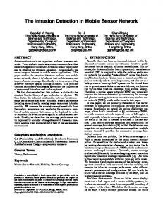
In this section, we focus on the case where the cats have a longer sensing range than the mouse. In this case, the mouse is always detected before it can see the cat; hence, the mouse can be considered a “blind” mouse. A. Strategy of the mouse Since a blind mouse cannot sense a cat’s actual movement, the mouse is assumed to have some high level information about the cats’ movements in order to avoid detection. Specifically, we assume that the mouse knows the statistical movement model and the sensing range Rc of the cats. Based on the information, we estimate the probability of finding at least one cat for any position in the network, and design the best strategy for the mouse accordingly. With a sensing range Rc , each cat controls a circular region of area πRc2 . Roughly speaking, each cat controls a square region—which we call a cell—of size s × s, √ with s = πRc . We then consider the network area to consist of X/s by Y /s disjoint cells, with each cat controlling the cell in which it is currently located. The presence matrix Π is defined such that Π[x, y] denotes the probability that at least one cat is present in cell i = (x, y) at any instant (when the context is clear, we use πi as a shorthand for Π[x, y]); note that Π can be obtained since the cats’ movement model is known. For instance, Figure 1 shows the presence matrix for a single cat (i.e., Nc = 1) moving under the random waypoint (RWP) algorithm [1] in a network area of 10 × 10 cells. 0.02 0.018 0.016 0.014 0.012 Probability
0.01 0.008 0.006 0.004 10
0.002 7
0 1
2
3 X
4
4 5
6
7
8
9
Y
1 10
Fig. 1. The presence matrix with 10 × 10 cells for a single cat moving under the RWP algorithm in the network area. The mean of the probabilities is 0.01, while the standard deviation is 0.012.
Remark: If Nc > 1 and the cats are moving independently under the same movement model, it is easy to obtain the presence matrix Π for Nc cats based on
4
the presence matrix of a single cat. In particular, let pi be the presence probability of one cat in cell i. Then, the presence probability for at least one of the Nc cats appearing in cell i isPπi = 1 − (1 − pi )Nc . Also note that P and i πi ≤ Nc . i pi = 1
Dynamic programming solution for the best strategy: Given the presence matrix Π, what strategy should the mouse use to maximize the expected detection time? One simple greedy strategy is for the mouse to continually move to the neighboring cell having the lowest presence probability, and stop moving when all the current cell’s neighbors are more dangerous (i.e., they have a higher presence probability). The intuition is that the expected detection time will immediately increase whenever the mouse visits a new cell along the path. However, the greedy strategy may not always find the best path for the mouse, since it prevents the mouse from considering those paths that temporarily access a more dangerous neighboring cell but will eventually lead to a safe network location. For example, in Figure 2, the greedy strategy suggests that the mouse should move from cell a to cell c along the illustrated path, and finally stop at c. However, under most values of the mouse’s and cat’s speeds, the optimal path for the mouse is to move from cell a to cell b. 0.0005
0.0005
0.0005
0.0075
0.0075
0.0075
0.0075
0.0005
0.0075
0.03
0.03
0.03
0.03
0.03
0.03
0.0075
0.0075
0.03
0.021
0.023
0.025
0.03
0.0075
0.02
ALGO()
Initialize E[Tidetect ] of each cell i with E[Tistay ] For each cell i, mark i as its next step Put each cell i into a max-heap using E[Tidetect ] as key while heap is not empty Extract cell i from heap with largest key for each neighbor cell k of i move ] Calculate E[Tk,i move ] > E[T detect ] if E[Tk,i k move ] Update cell k’s key E[Tkdetect ] to E[Tk,i Re-insert cell k into the max-heap Mark i as k’s next step end if end for end while
Fig. 3. DP
ALGO :
A dynamic program for the mouse’s best strategy.
In the algorithm, we initialize E[Tidetect ] to E[Tistay ] for each cell i in Line 1, and insert the cell into a heap with key value E[Tidetect ], sorted in decreasing order (Line 3). For each iteration (Lines 4-14), we first extract the cell i with the largest key value from the heap, so that the value E[Tidetect ] will not be further updated. Then, for each neighboring cell k of i, we update E[Tkdetect ] move to E[Tk,i ] if the latter value is larger, meaning that the mouse starting at cell k can benefit from moving to cell i. If there was an update, we reinsert cell k into the max-heap with the updated key value (Lines 6-9). Also, we mark cell i to be the next cell to move to when the mouse is in cell k (Line 10).
b
a 0.0075
0.03
0.018
0.03
0.03
0.03
0.03
0.0075
0.0075
0.03
0.03
0.016
0.014
0.01
0.03
0.0075
Theorem 1. DP ALGO is an optimal algorithm for the mouse, against any presence matrix Π. "hill" of high probability optimal escape path local greedy escape path
c 0.0075
0.03
0.03
0.03
0.03
0.03
0.03
0.0075
0.0075
0.0075
0.0075
0.0075
0.0075
0.0075
0.0075
0.0075
Fig. 2.
DP 1 2 3 4 5 6 7 8 9 10 11 12 13 14
A greedy movement strategy may not be optimal.
To avoid missing the optimal path, we apply the dynamic program DP ALGO as shown in Figure 3. In the figure, there are three groups of variables, move namely E[Tidetect ], E[Tistay ], and E[Tk,i ]. The value detect E[Ti ] represents the expected detection time when the mouse starts at cell i and uses the best path among the paths considered so far. This value will be updated as the algorithm proceeds, and will eventually hold the desired expected detection time when the mouse uses the best path among all possible paths. The value E[Tistay ] denotes the expected detection time when the mouse starts at cell i and stays there forever. Finally, the value move E[Tk,i ] denotes the expected detection time when the mouse starts at cell k, moves to a neighbor cell i, and follows the best strategy once it reaches cell i.
Proof: In general, a mouse strategy specifies what the mouse should do when it is in a certain cell (whether to stay or move to a particular adjacent cell). We shall argue that the action determined by DP ALGO at each cell is optimal. In particular, we shall prove by induction the following: the jth best cell is extracted in Line 5 of the jth iteration, whose optimal action is to move to its next step.2 In addition, upon the extraction of any cell i, E[Tidetect ] will be correctly set to the expected detection time under any optimal mouse strategy. In the first iteration, the cell i1 with the largest E[T detect ] is extracted. This cell must be the one with the largest E[T stay ], so that it must be the best cell. Here, we determine that the mouse should “stay” (since its next step is itself), and such an action is clearly optimal. Next, suppose that the j − 1 best cells are extracted in the first j − 1 iterations. For the jth best cell ij , we can see that its optimal action is either to stay, or to move to the best adjacent cell (if it yields a longer expected detection time). Note that if the latter case is true, such an adjacent cell, say w, must be one of the best j − 1 2 Here, the jth best cell is the cell which, when chosen as the initial position, has the jth longest expected detection time, under an optimal mouse strategy.
5
cells, so that E[T detect ] of ij is set to the optimal value upon w’s extraction (Lines 6-13). Then in both cases, the jth best cell must have the largest E[T detect ] among all the remaining cells at the jth iteration, so that it will be extracted. Furthermore, its optimal action and the corresponding E[T detect ] are set correctly as required. This completes the induction step. It remains to show how to compute E[Tistay ] and move E[Tk,i ]. To do so, we use a concept called the cell sojourn time, which is the length of time that a cat stays in the current cell before it moves to a neighboring cell. The expected sojourn time, denoted by E[T s ], can be calculated since the cats’ movement model is known. For the purpose of estimation, we may assume that the status of whether any cat is present in a certain cell is unchanged during the time interval [ℓt, (ℓ + 1)t), for t = E[T s ] and any non-negative integer ℓ. Then, we can estimate E[Tistay ] by E[Tistay ] ≈
∞ X ℓ=0
(ℓE[T s ])πi (1 − πi )ℓ = E[T s ]/πi . (1)
move To calculate E[Tk,i ] based on the optimal detect ], we let tk,i be the time taken by the mouse E[Ti to move from (the center of) cell k to (the boundary of) cell i. Then, the mouse will either be caught in cell k, or it can reach cell i so that it is expected to be caught after another time of E[Tidetect ]. The probability that it can reach cell i without being caught can be estimated by s (1 − πi )tk,i /E[T ] . Using an approach similar to the one move used to estimate E[Tistay ], we can estimate E[Tk,i ] by
place for the mouse to stay, which reduces the (worstcase) expected detection time of the mouse. In fact, the uniform presence matrix is an optimal strategy for the cats, as shown in the following theorem: Theorem 2. When the mouse applies DP ALGO, an optimal strategy for the cat is to set its presence matrix uniform. Proof: Let M denote an arbitrary presence matrix, and U denote the uniform presence matrix. When the mouse applies DP ALGO, we let tM and tU denote the expected time for the cat to catch the mouse when using M and U , respectively. We shall show that tU ≤ tM , thus proving the theorem. To link the two quantities, we consider a further expected time t′M , which corresponds to the case that the cat uses presence matrix M , and the mouse simply never moves. It is easy to see that t′M ≤ tM , since if the mouse never moves, it will never improve (i.e., lengthen) the detection time. On the other hand, when the network has x × y cells, X 1 1 t′M = × (2) xy M [i, j] i,j X 1 1 ≥ × (3) xy U [i, j] i,j = tU ,
(4)
so that tU ≤ t′M ≤ tM . Here, Eq. 3 follows from the fact that for any a, b > 0, (1/a) + (1/b) ≥ 1/((a + b)/2) + 1/((a + b)/2). The presence matrix can be generalized for Nc cats, in which case each cell is associated with a probability that Z tk,i at least one cat is present in the cell. The sum of these tk,i t πi (1 − πi ) E[T s ] tdt + (1 − πi ) E[T s ] (E[Tidetect ] + tk,i ) probabilities can be as large as Nc , which is achievable 0 when the cats are always in disjoint cells. When the It can be shown that the dynamic program has time network has x × y cells, and each cell is associated complexity O(n log n), where n = XY /s2 . We omit the with a probability Nc /(xy), we call this presence matrix analysis due to limited space. maximum-uniform. Repeating the arguments in Theorem 2, one can easily show the following result: B. Strategy of the cats Based on the strategy in the previous section, the mouse may eventually move to a safer position that has a lower cat presence probability than its current position, thereby maximizing the expected detection time. Hence, the best strategy for the cats seems to maximize the minimum presence probability among all the cells in Π. The maximin strategy implies that when the cats are moving independently under the same movement model, the best choice for each cat is to move in a way such that the presence probability is the same in each cell. (We call the resulting presence matrix in which all the entries have equal values a uniform presence matrix.) With a uniform presence matrix, there is no particularly safe
Corollary 1. When the mouse applies DP ALGO, an optimal strategy for Nc cats is to set the presence matrix maximum-uniform. Theorem 3. Nash equilibrium is achieved when the mouse applies DP ALGO and the cats apply the maximum-uniform presence matrix. Proof: A direct consequence of Theorem 1 and Corollary 1. To yield a uniform presence matrix in the single-cat case, one simple example movement is to sequentially and circularly scan all the network cells. However, the deterministic nature of the cat’s movement may allow
6
the mouse to accurately predict where the cat will be and therefore easily avoid it. Hence, we will present in Section V-B a probabilistic movement strategy that can achieve a presence matrix close to being uniform. As mentioned, when there are Nc cats, it is better for them to move in disjoint areas of the network, as the sum of πi in the presence matrix is equal to Nc , which is greater than the sum of πi if the cats move independently. This suggests that if the cats are allowed to move in a coordinated way, we should always assign them to monitor disjoint parts of the network. Accordingly, the best strategy for the cats is to divide the network into Nc equally sized partitions, in which one cat moves within one partition optimally to yield a maximum-uniform presence matrix. V. The Seeing Mouse (Rc < Rm ), Independent Cats In this section, we discuss the case when the mouse has a larger sensing range than the cats. In this case, once a cat enters the mouse’s sensing range, the mouse can know the cat’s movement in advance without being detected. We focus on the case that the mouse’s speed is less than the cats’ (i.e., Vm < Vc ); we believe that the other case is not as interesting since intuitively, the faster mouse can always avoid being detected. In the following, we first propose a strategy for the mouse to escape from the cats based on such advance knowledge. We then discuss some possible strategies that the cat may use to reduce the detection time, knowing that the mouse may run away when it sees the cat. We assume in this section that the cats act independently. A. Strategy of the mouse We first study the special case in which there is only one cat in the network. Then, we generalize the strategy to the case of multiple cats. Avoiding a single cat: When the mouse tries to escape from a cat, it is better if it can move in a direction β such that the minimum distance between the mouse and the cat (assuming that the cat does not change its speed and moving direction) in the future is as large as possible. Let C and M be the current positions of the cat and the mouse, respectively. Let α be the moving direction of the cat. Then, the position of the cat at time t, denoted by C(t), can be expressed as C + (Vc cos α · ˆı + Vc sin α · ˆ) t.
(5)
Similarly, if the mouse chooses to move in a direction β at a speed of Vm , the position of the mouse at time t, denoted by M (β, t), can be expressed as M + (Vm cos β · ˆı + Vm sin β · ˆ) t.
(6)
γ is maximized when this angle is π/2
Mouse V Vm -Vc
to maximize γ
Mouse Vm
γ
-Vc β *=α+arccosVm
Vc
Vc
Vc
α
Cat
α
Cat
~ = V~m − V~c (a) V
Fig. 4.
γ
β*
(b) To maximize γ.
The mouse’s choice of β ∗ to maximize γ.
Then, the distance between the cat and the mouse at time t is equal to d(β, t) = kC(t) − M (β, t)k. By differentiating d(β, t) with respect to t, we can find the minimum distance between the mouse and the cat for t ≥ 0. We denote such a distance by d∗ (β). In other words, in order to maximize the distance from the cat in the future, the mouse should find a direction β ∗ such that β ∗ = argmax d∗ (β). (7) β
Remark: In fact, by a simple geometric argument, the optimal β ∗ for the single-cat case can be easily obtained. Essentially, the cat is moving in a vector V~c = Vc cos α · ˆı + Vc sin α · ˆ, while the mouse choosing a direction β is moving in a vector V~m = Vm cos β · ˆı + Vm sin β · ˆ. Equivalently, we may assume that the cat is stationary, ~ = V~m − V~c while the mouse is moving in a direction V towards the cat. To maximize the distance between the cat and the mouse, we want (the absolute value of) the angle γ between V~ and the vector from the mouse to the ~ −M ~ ) to be as large as possible. As shown cat (i.e., C in Fig. 4, we have � � Vm β ∗ = α + arccos . (8) Vc Avoiding multiple cats: We have shown how the mouse can choose the optimal direction β ∗ when there is only one cat. In the case of multiple cats, we need to find a β ∗ that maximizes the minimum distance to all the cats in the future. Using similar notations, we let d∗i (β) denote the minimum distance between the mouse and the ith cat in the future, assuming that the mouse is moving in the direction β. In other words, if there are j cats within the sensing range of the mouse, we have n o β ∗ = argmax min d∗1 (β), d∗2 (β), . . . , d∗j (β) . (9) β
Notice that in the case of multiple cats, a direction β that maximizes the minimum distance for one cat does not necessarily yield a short minimum distance for another cat. Finding the optimal β ∗ may require us to consider all the intersections between any two of the j
7
curves d∗i (β), so as to decide the best direction; in the worst-case, there can be Ω(j 2 ) such intersections. An alternative way is to obtain a close estimation of β ∗ , by choosing a small angle δ and computing all d∗i (β) values for β = 0, δ, 2δ, 3δ, . . . , ⌊2π/δ⌋δ, and then finding β ∗ based on only these values. The drawback of the above estimation is that we may miss the optimal β ∗ when it is not a multiple of δ. However, there are only O(j/δ) values to compute, and the simplicity of the method will usually allow us to obtain a good enough β ∗ efficiently in practice. Degree of freedom and a revised strategy: In general, it is not necessary for the mouse to choose the optimal direction β ∗ to avoid being caught. It is because when choosing a direction β, a mouse will not be detected as long as its minimum distance to all the cats in the future is larger than the cats’ sensing range Rc . Hence, the mouse may choose a direction from a feasible set B such that � � ∗ (10) B = β min {di (β)} > Rc . 1≤i≤j
Thus, the larger the size of B is, the more directions the mouse can choose from, so that it is more likely for a mouse to escape successfully. Note that the mouse may have fewer choices when it is located at the boundaries or the corners of the network area. In fact, if the cats move under the RWP algorithm and the mouse uses the above strategy to escape (so that it chooses to move at an angle of β ∗ when one or more cats are around, and stops moving when no cat is around), the results in Fig. 5 show that the mouse will likely be “pushed” to the corners/boundaries of the network, and then be caught there.
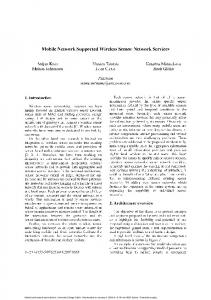
may be offset by the predominant presence of the cats near the center. B. Strategy of the cats Since a cat knows that the mouse may see it before it sees the mouse, the cat may assume that the mouse will try to run away from it in advance. One logical choice of strategy for the cats is then to visit more frequently the center region of the network, where the mouse has more freedom to move and escape. As shown in Figure 1, a cat can achieve the goal of visiting the center region more often by playing the RWP strategy. On the other hand, the cats may also benefit from a movement strategy that will yield a uniform presence matrix, so that they will eliminate safe havens for the mouse to hide in. As both kinds of strategy have their merits, we will compare their empirical performance in Section VII. We use the following simple random algorithm, which we call the bouncing strategy, for the cats to approximate closely the uniform presence matrix. In the algorithm, a cat moves in a straight line until it hits the boundary or a corner of the network area. Whenever it reaches the boundary/corner, it selects a direction randomly and uniformly from all the feasible directions and proceeds to move in the selected direction. Figure 6 shows the presence matrix for a cat moving under the bouncing model. Alternative algorithms are known that can provably achieve uniform presence for the cats [2], [10]. 0.018 0.016 0.014 0.012 0.01 Probability 0.008 0.006 0.004 9 0.002
7 5
0 1
2
3
Y
3 4
5 X
6
7
8
9
1 10
Fig. 6. The presence matrix with 10×10 cells for a single cat moving under the bouncing strategy in the network area. The matrix is close to the uniform presence matrix. Fig. 5. The black dots show the positions where the mouse is detected in 50,000 simulation runs. The mouse is caught at the the network corners and boundaries in most cases.
This leads to a revised strategy for the mouse to always move towards the center region of the network whenever there is no cat detected within its sensing range. We call this the centric strategy. Our results in Section VII show that the centric strategy works well among other strategies evaluated, when the cats have a uniform presence matrix. When the cats use RWP, however, the mouse’s degree of freedom at the center
Remark. In the seeing mouse case, the cats have no information about the mouse during the game. An optimal cat strategy can be defined in the minimax sense, i.e., the optimal strategy minimizes the hypothetical expected detection time over all possible mouse strategies. However, given that there are infinitely many possible mouse strategies, and that the cats have no information about what the mouse might choose, we conjecture that finding the optimal cat strategy is undecidable. Hence, we propose only heuristic cat strategies in the above discussion.
8
VI. The Seeing Mouse and Coordinated Cats In this section, we consider the seeing mouse, and a network of cats who may coordinate their movement to maximize their ability to detect the mouse. We consider two coordination approaches. The first one is enabled by the cats’ ability to see each other within their sensing range. The second one is enabled by the cats’ additional ability to communicate over a wireless range of Wc . A. Sensing-based coordination (SBC) When a cat moves close to other cats, their sensing regions overlap, which results in inefficient use of the sensing resources. Such an overlap can be detected partially by the cats involved. Specifically, they can see each other when they fall within the sensing range of each other. When that happens, the cats can try to move away from each other in order to reduce the overlap in spatial coverage. We call such a coordination approach sensing-based coordination (SBC). In SBC, a cat moves according to the usual algorithm (e.g., bouncing or RWP) until it detects one or more other cats within its sensing range. When that happens, the first cat will try to maximally avoid the other cat(s), i.e., to minimize the expected future overlap in coverage by the cats. This can be done by using the same algorithm that a seeing mouse uses to avoid a detected cat, namely the geometry-based algorithm presented in Section V-A. According to the algorithm, the cat computes the optimal β ∗ in order to optimally move away from the other cat(s). B. Communication-based coordination (CBC) In SBC, the cats coordinate by observing each other’s movements only. If the cats can also communicate over a wireless channel of range Wc , they can further coordinate their strategies to reduce the expected detection time of the mouse. First, if Wc > Rc , the coordination can occur sooner and therefore be more proactive. Second, the cats can actively exchange information about their strategies (e.g., the planned future movements), instead of using passive observations only. We call such a coordination approach communication-based coordination (CBC). The CBC algorithm we use (Fig. 7) is motivated by the observation in Section V-A about the importance of the mouse’s degree of freedom in enabling its escape strategy. Specifically, we aim to allow the cats to team up and form a cohort in searching for the mouse. The concerted efforts of the cohort members will then form a larger barrier that limits the mouse’s degree of freedom in passing the barrier. The algorithm in Fig. 7 allows cohorts to form in an opportunistic manner. We assume that each cat’s plan of movement consists of a sequence of trips, and the destination of one trip is the starting
point of the next trip, and so on. We call the destination of a trip a waypoint. Cohorts are then formed as follows. A cat, say C, that is acting independently (i.e., not in any cohort currently) will continuously attempt to establish wireless communication with another cat, which happens when the other cat, say D, comes within a distance of Wc of C. With a probability of 1 − pf , C will ignore the communication and repeat looking for a new cat for communication. Otherwise (i.e., with a probability of pf ), C asks D about its current destination waypoint. C will then abandon its current waypoint and join D by adopting a new waypoint that is “close to” D’s waypoint. (The “close to” notion will be made precise in the following.) Once C decides to join D and is on its way to the new waypoint, it considers itself committed and will not attempt to establish communication with other cats. Once C has reached the new waypoint, however, it will repeat the procedure of entering another cohort. Notice that while a more effective barrier is formed by a larger cohort, a larger cohort size will result in a fewer number of cohorts since the number of cats is fixed. A small number of cohorts limits the ability to spread out the cats over different parts of the surveillance area where the mouse may be found. Hence, a tradeoff between the cohort size and the number of cohorts is useful. The pf parameter aims to provide this tradeoff, in which a larger pf value is more likely to produce larger cohorts. Notice also that, while the teaming of cats forms a useful barrier against the escape of the mouse, it is also important to avoid the inefficient coverage overlap that can happen with uncontrolled teaming. This is the reason when C decides to follow D in the above example, it does not try to go to the same waypoint as D, but selects a new waypoint close to D’s. Specifically, the new waypoint is computed as follows: C selects a waypoint that is 2Rc away from D’s and whose direction from D’s is perpendicular to D’s movement vector. The waypoint selection strategy is illustrated in Figure 8. Notice that two cats having the same speed are likely to arrive at the new waypoints at about the same time, and will form a maximum barrier against the mouse’s escape. In general, we have conjectured about the hardness of the optimal independent cat strategy against the seeing mouse. The problem becomes more difficult when coordinated cats are considered. A number of related heuristic algorithms for coordination are known [3], [7], [13]. Our goal in this paper is not to extensively cover the design space of CBC, but to contrast between the SBC and CBC approaches, and evaluate how the cats may use coordination to improve against effective mouse strategies identified in our previous discussions.
9
Start
Establish communication with another cat
No
strategy, in three sets of runs. From the table, notice that the mouse can achieve a significantly higher average detection time by playing the dynamic programming strategy, as the analysis in Section IV-A shows.
Following another cat?
Yes
Is this cat in set G?
Yes
Communication established?
No
Reached waypoint?
No
Yes
No
Yes
Follow?
Change waypoint
Select a new waypoint and clear set G
No
Move
Add cat to set G End
Fig. 7.
The communication-based coordination (CBC) approach.
Fig. 8. Coordinated waypoint selection to minimize coverage overlap in CBC.
VII. Experimental Results A. The blind mouse: Rc ≥ Rm
This section evaluates the case of a blind mouse. Unless otherwise specified, we report average results over 100 simulation runs, each lasting 200,000 seconds. We omit the standard deviations, because they are very small compared with the means. In the discussion, when a node deterministically cycles through all the cells in the network area, we will refer to the movement as the scan strategy. 1) Benefits of dynamic programming solution for the mouse: We compare the performance of different movement strategies for the mouse in Table I. In the table, the column “DP” refers to the case when the mouse determines its movement by the dynamic programming strategy in Section IV-A. The mouse is initially located at the center of the network area. The column labeled “Stay” in Table I is used for baseline comparison, and refers the to case when the mouse simply stays at its starting position (i.e., it does not move at all afterward). The experiments use one cat. Its movement strategy is shown as the rows of Table I, and is chosen to be (1) the uniform scan strategy, (2) the bouncing strategy in Section V-B, and (3) the random waypoint (RWP)
Mc \ Mm uniform scan Bouncing RWP
DP 1083.26 628.66 2823.26
RWP 415.31 442.23 271.73
Stay 511.50 305.03 226.13
2) Uniform presence matrix benefits the cat: The “DP” column in Table I also shows how a uniform presence matrix may benefit the cat. From the results, notice that the simple scan strategy can greatly reduce the detection time compared with the non-uniform RWP strategy. However, as discussed in Section IV-B, the deterministic nature of the scan strategy may allow the mouse to predict where the cat will be in advance and thus effectively avoid the cat. To avoid the problem, the bouncing strategy can closely approximate the uniform presence matrix without being deterministic. 3) Effects of the cat’s sensing range: In this experiment, there are one cat and one mouse moving in a 500 m × 500 m network area. The mouse plays the dynamic programming strategy. The cat uses (1) the RWP strategy and (2) the bouncing strategy, in two different runs. We measure the average detection time of the mouse for different sensing ranges, Rc , of the cat. Fig. 9 shows that as Rc increases, the average detection time decreases as an inversely proportional function of Rc , showing that the cat’s ability to detect the mouse increases proportionally to its sensing capability. 60000 Average detection time (s)
Yes
TABLE I AVERAGE DETECTION TIME ( IN S ) FOR DIFFERENT CAT AND MOUSE MOVEMENT STRATEGIES IN A 500 M BY 500 M NETWORK . Vc = Vm = 10 M / S , Rc = 25 M , AND THE MOUSE IS INITIALLY LOCATED AT THE CENTER OF THE NETWORK .
RWP Bouncing
50000 40000 30000 20000 10000 0 0
10
20
30 Rc (m)
40
50
60
Fig. 9. Average detection time (in s) of the mouse versus the cat’s sensing range Rc (in m); Vc = Vm = 10 m/s.
4) Number of cats: In this experiment, we measure the average detection times when the number of cats is varied. The network area is 500 m × 500 m, and the sensing range of each cat is 25 m. Similar to the previous experiment, the mouse plays the dynamic programming strategy, while the cats independently play either the RWP or the bouncing strategy. Fig. 10 shows that as the number of cats increases, the average detection time
10
decreases, approximately like inversely proportional to Nck , where k is a constant slightly larger than one. Average detection time (s)
3000
RWP Bouncing
2500 2000 1500 1000 500 0 0
10
20
30
40
50
Nc
Fig. 10. Average detection time (in s) versus the number of cats Nc in a 500 m by 500 m network area; Vc = Vm = 10 m/s.
5) Effects of Vc and Vm on dynamic programming solution: In this experiment, there are one cat and one mouse. We illustrate how the expected detection time of the mouse varies with different speeds Vc and Vm of the cat and the mouse, respectively. The mouse plays the dynamic programming strategy. Fig. 11 shows that the average detection time is reduced when the cat moves faster (i.e., Vc is higher). This is because a faster cat can cover a larger area in the same amount of time. Notice also that the detection time increases when the mouse moves at a higher speed. This is because a faster mouse can move from its current position to a safe position more quickly, and benefit from staying in the safe position longer. We also find that the mouse can benefit more from moving at a higher speed, if the cat itself is moving at a higher speed. This shows that a fast cat will force the mouse to be fast to avoid detection.
Average detection time (s)
3000 2500 2000 1500 1000 500 0 0
0 20 40
50
60 80 100
100
Vm (m/s)
Vc (m/s)
Fig. 11. Average detection time (in s) versus the speeds (in m/s) of the cat and the mouse in a 500 m by 500 m network. Rc of the cat is 15 m.
We further show that the path of movement computed by the dynamic program in Figure 3 is dependent on the speed of the mouse. In Figures 12(a) and 12(b), the gray level represents the cat’s presence probability (the darker an area, the lower the cat’s presence probability in the area). The cat has a speed of 10 m/s. The arrows in the figure show the escape paths of the mouse in a 500 m × 500 m network area divided into 10 × 10 cells. The paths when the mouse has a speed of 10 m/s are shown in Figure 12(a). The paths when the mouse has
a higher speed of 15 m/s are shown in Figure 12(b). In the figure, cells j and k are cell i’s neighbor. Cell k is safer than j, and both of them are safer than i. Assume that the mouse is currently in cell i. Notice that when the mouse has the lower speed, it will move to the less safe neighbor j because j is closer in distance than k. Choosing the closer neighbor allows the mouse to leave the more dangerous cell i soon (considering that the mouse moves slowly). When the mouse has the higher speed, it can afford to move a longer distance before leaving cell i. Hence, it will choose to move directly to the safer neighbor k although k is farther away.
i j k
0.0030
0.0115
i j k
0.0200
(a) Vc = Vm = 10 m/s.
0.0030
0.0115
0.0200
(b) Vc = 10 m/s, Vm = 15 m/s.
Fig. 12. Escape paths calculated by the algorithm MaximizeDetectTime() for a 500 m by 500 m network area divided into 10 by 10 grids, for different speeds of the mouse.
B. The seeing mouse (Rm > Rc ), independent cats We now evaluate the case of a seeing mouse, when the cats do not coordinate. In the experiments, unless otherwise specified, the cats play the bouncing strategy and Rc = 5 m and Rm = 10 m. We report maximum, minimum, and average results over 5,000 simulation runs within a 100 m by 100 m area. 1) Movement direction β for the mouse: In this experiment, we report the optimal direction β ∗ calculated by Eqn. 9 to maximize the minimum distance between the cats and the mouse. We use Vc = Vm = 5 m/s. There are six cats and one mouse. Figure 13, shows the minimum distance of the mouse from each cat, as a function of the mouse’s direction of movement β. In the figure, the thick line shows the minimum distance of the mouse from any of the cats. Of the thick line, the dark segment shows the range of the movement angles over which the minimum distance (from any of the cats) is maximized, and thus gives the range of the optimal maximin solutions computed. Any angle that falls within the range can be used by the mouse as its optimal movement direction. 2) Effects of Rc and Nc : In this experiment, we use ten cats, and show how Rc can affect the range of maximin solutions available to the mouse as it tries to find an optimal angle of movement. In Figure 14, we report the fraction of the movement angles that are in
11
Minimum distance between cat and mouse (m)
90 Cat 1 Cat 2 Cat 3 Cat 4 Cat 5 Cat 6 Minimum Maximin
80 70 60 50 40 Range of maximin solutions 30
Minimum distance to all the cats 20 10 0
0
50
100
150 200 Beta (degree)
250
300
350
Fig. 13. The minimum distance d∗ (β) calculated by Equation 9 between six cats and one mouse as a function of the mouse’s movement direction β. The cats and the mouse are initially randomly placed in a 100 m by 100 m network.
the feasible set B (defined by Equation 10) as a function of Rc . The results show that the fraction of feasible solutions decreases like exponentially as Rc increases (up to Rm ), showing that the mouse’s degree of freedom in choosing a solution is severely restricted as the cat’s sensing capability increases. 1
Fraction of feasible solutions
0.9 0.8 0.7 Maximum
0.6 Median 0.5 0.4
Maximum
0.3
Mean
Mean 0.2
Median
0
Minimum
Minimum
0.1 0
10
20 30 Sensing range (m)
40
50
Fig. 14. The fraction of feasible solutions calculated by Equation 10 as a function of the cat’s sensing range Rc . Ten cats are randomly placed in a 100 m by 100 m network. Rm = ∞.
We next consider the effects of Nc , the number of cats. In Figures 15 and 16(a), we show that as Nc increases, both the optimal minimum distance (of the mouse) from any of the cats and the average detection time decrease. 140 Maximum Mean Median Minimum
Maximin distance to any cats (m)
120 100 80 60 40 Minimum
20 0
0
20
40 60 Number of cats
80
100
Fig. 15. Statistics of the maximin distance of the mouse from any of the cats, as a function of the number of cats Nc . Both the cats and the mouse move according to the bouncing strategy in a 100 m by 100 m network area.
3) Effects of Rm and Vm : We show the impact of the mouse’s sensing range Rm on the detection time in Figure 16(b). As Rm increases, the mouse can detect the cats earlier and are better able to make the necessary moves to avoid the cats. Hence, the detection time increases significantly at first. As Rm increases beyond 9 m, however, the detection time does not change much. This shows that information about the cats that are far away (as captured by a large sensing range Rm ) may not be that useful to the mouse in determining its immediate course of action. The results in Figure 16(c) show that the detection time generally increases as the mouse’s speed increases. This is because a faster mouse can avoid the cats more quickly and allow itself more choices of the optimal movement direction β ∗ . 4) Comparison of different strategies: We discussed the bouncing and centric strategies for the seeing mouse in Section V-A. These strategies define what the mouse should do when it sees no cat within its sensing range. An alternative strategy in such a situation is for the mouse to simply stay where it is, presumably to conserve energy, and we call it the static strategy. In this experiment, we compare the performance of these strategies for the mouse, while ten cats in the network play either the bouncing or the RWP strategy. The average detection time results are shown in Fig. 18. As a baseline case for comparison, we also show a “stay” strategy in which the mouse simply stays at its starting position; i.e., the mouse never moves (i.e., Vm = 0) and does not apply Equation 9 to determine its angle of movement. From Fig. 18, notice that bouncing is the best strategy for the cats, where their presence matrix is approximately uniform. For the mouse, its best strategy depends on the cats’ strategy. When the cats play the RWP strategy, the best strategy for the mouse is bouncing. When the cats play the bouncing strategy, the best strategy for the mouse is centric. We further quantify how deviations from the center position by the mouse will impact the average detection times in this case. We use an off-centric mouse that will move to the closet point (from the mouse’s current location) that is k distance away from the center, and vary k in a set of experiments. (When k = 0, we have a centric mouse.) The results in Figure 17 verify that a mouse moving closer to the center can increase the average detection time when the cats have a uniform presence matrix. The above results show an interesting interplay between the cats’ and the mouse’s movements. When the cats use the bouncing strategy, the mouse benefits by moving toward the center of the network, where it has a higher degree of freedom as discussed in Section V-A. However, this higher degree of freedom is offset, in the case of this experiment, when the cats use the RWP
12
4500
2000 Mean Median Minimum Maximum
3000
Detection time (s)
Detection time (s)
3500
2500 2000 1500
Maximum
Mean
Mean
1600
Median
1400
Minimum
2000
Median Minimum
1200 1000 800
1500
1000
600
1000
400
500
Minimum
500 0
2500 Maximum
1800
Detection time (s)
4000
Minimum
Minimum 200
0
5
10 Number of cats
15
0
20
0
2
4
6 8 10 12 Mouse sensing range (m)
(a)
14
16
18
0
0
5
10 Mouse speed (m/s)
(b)
15
20
(c)
400
1800
350
Average detection time (s)
Average Detection Time (s)
Fig. 16. Statistics of the detection times as a function of (a) Nc , (b) Rm , and (c) Vm . The cats randomly move in a 100 m by 100 m network. Both the cats and the mouse use the bouncing strategy.
300 250 200 150 100 50 0 0
10
20
30
40
50
Distance away from the center (m)
1600 1400
RWP Cat
RWP/SBC Cat
Bouncing Cat
Bouncing/CBC Cat
RWP/CBC Cat
1200 1000 800 600 400 200 0 Bouncing
Centric
RWP
Seeing Mouse Strategies
Fig. 19. Average detection time comparison of the SBC and CBC coordination approaches, for different combinations of the mouse and basic cat movement algorithms.
strategy to achieve a higher presence in the center area. The static strategy performs the worst in all of the cases measured.
coordination, Wc and pf are set to be 10 m and 0.7, respectively, unless otherwise stated.
RWP Mc Bouncing Stay
Static
Centric
1600 1400 1200 1000 800 600 400 200 0 Bouncing
Average detection time (s)
Fig. 17. Average detection times of off-centric mouse strategy for different values of k in a 100 m × 100 m surveillance area. Vc = Vm = 10 m/s, Rc = 5 m, Rm = 10 m, Nc = 10.
Mm
Fig. 18. Average of the mouse detection time (in s) under different strategies for the cats and the mouse in a 100 m by 100 m network. V c = 5 m/s, V m = 10 m/s, Rc = 5 m, and Rm = 10 m.
C. Seeing mouse and coordinated cats We evaluate the performance of the coordination approaches in Section VI for the cats playing against a seeing mouse. We use 10 cats in a surveillance area of 100 m by 100 m; the cats and the mouse all have the same speed of 10 m/s; the cat and mouse sensing ranges are 5 m and 10 m, respectively. When there is no cat within the sensing range of a seeing mouse, the mouse plays the bouncing, centric, or RWP strategy, and we correspondingly call it the bouncing, centric, or RWP mouse. For each set of parameters, we report the average detection times of 1000 simulation runs in Figure 19. The error bars show the 95% confidence interval. For CBC
The results in Figure 19 show that the coordination approaches are highly useful for the RWP cats, but have relatively small effects for the bouncing cats. This is because the bouncing cats are evenly spread out in the surveillance area as evidenced by their uniform presence matrix. For SBC, they get few chances to meet in the first place, and therefore do not need help from SBC to move away from each other. For CBC, the cats similarly have few chances to get close and attempt the opportunistic clustering if the communication range is small. If the communication range becomes larger, the pairing opportunities increase. However, the cats who decide to cluster may arrive at the coordinated waypoints far apart from each other, which reduces the effectiveness of the barrier formed. For the RWP cats, SBC coordination reduces the average detection time by at least 161% (against the centric mouse), by decreasing the overlap in spatial coverage relative to the uncoordinated cats. Compared with SBC, CBC coordination reduces the average detection time by at least 384% (against the bouncing mouse). This shows the additional benefits of teaming up the cats to reduce the mouse’s degree of freedom in evading the cats. The benefits are particularly obvious for the centric mouse and the RWP mouse, as the two kinds of mouse do tend to concentrate in the center and can maximally benefit from the high freedom of movement there if not countered by the cats’
13
coordination strategy. Figure 20 shows the impact of Wc on the average detection time of CBC, for the mouse strategies of bouncing, centric, and RWP, respectively, when pf is fixed at 0.7. We omit the standard deviations as they are small compared with the averages. As previously explained, CBC coordination is highly useful for the RWP cats, but has less effect for the bouncing cats. For the RWP cats, the performance of CBC is highly dependent on the communication range. In general, it increases quickly as Wc increases, up to a value of 2Rc , after which further increases in Wc have little impact. Notice also that the RWP/CBC cats are most effective against the centric mouse. This is because whereas the centric mouse aims to achieve a high degree of freedom to escape at the center, the CBC approach is specifically designed to counter that freedom. The design is so effective that whereas the RWP cats without coordination have far worse performance than the bouncing cats, the RWP cats can outperform the bouncing cats (with or without coordination) when CBC is enabled. For the centric mouse, when the communication range is large enough, RWP/CBC detects the mouse twice as fast as uncoordinated bouncing, and about 1.5 times faster than bouncing/CBC. The 3D plots in Figure 21 systematically explore the effects of Wc and pf on the average detection time, for 10 bouncing/CBC cats. The corresponding plots for 10 RWP/CBC cats are shown in Fig. 22. The evaluated mouse strategies are bouncing, centric, and RWP. Notice from the figures that a higher pf generally improves the performance of the coordination, over the entire range of Wc evaluated. This suggests the need to maximize the chance for the cats to work together in our experimental setting. For Wc , we point out that further to the observation we made about Fig. 8, the lowest detection time is achieved, across the space of the measurements, when Wc is about equal to 2Rc . Increasing Wc beyond 2Rc generally has little effect on the performance. The near optimality of Wc = 2Rc appears quite robust across a large number of experiments that we have run that are not reported in this paper.
expected time to detect the mouse. For a seeing mouse, we presented an efficient optimal algorithm based on geometric arguments that allows the mouse to maximally delay detection by reacting to the cats’ movements within its sensing range. We then discussed possible counter strategies by the cats to reduce the expected detected time. Furthermore, we discussed and evaluated SBC and CBC coordination approaches for the cats. R EFERENCES [1] J. Broch, D. A. Maltz, D. B. Johnson, Y. C. Hu, and J.Jetcheva. A performance comparison of multi-hop wireless ad hoc network routing protocols. In Proc. of MOBICOM, 1998. [2] T. Camp, J. Boleng, and V. Davies. A survey of mobility models for ad hoc network research. WCMC: Spec. issue on Mobile Ad Hoc Networking: Research, Trends and Applications, 2(5):483– 502, 2002. [3] J. P. Hespanha, H. J. Kim, and S. Sastry. Multiple-agent probabilistic pursuit-evasion games. In Proc. of IEEE Conf. on Decision and Control, 1999. [4] G. Hollinger and S. Singh. Proofs and experiments in scalable, near-optimal search by multiple robots. Robotics: Science and Systems, 2008. [5] R. Isaacs. Differential Games. Wiley, 1965. [6] V. Isler, C. Belta, K. Daniilidis, and G. J. Pappas. Hybrid control for visibility-based pursuit-evasion games. In Proc. of IEEE/RSJ Int. Conf. on Intelligent Robots and Systems, 2004. [7] V. I. S. Kannan and S. Khanna. Randomized pursuit-evasion with limited visibility. In Proc. of ACM-SIAM Symp. on Discrete Algorithms, 2004. [8] B. Liu, P. Brass, O. Dousse, P. Nain, and D. Towsley. Mobility improves coverage of sensor networks. In Proc. of MobiHoc, 2005. [9] N. Megiddo, S. L. Hakimi, M. R. Garey, D. S. Johnson, and C. H. Papadimitriou. The complexity of searching a graph. Journal of the Association for Computing Machinery, 35(1), 1988. [10] P. Nain, D. Towsley, B. Liu, and Z. Liu. Properties of random direction models. In Proc. of IEEE Infocom, 2005. [11] R. Teo, J. S. Jang, and C. J. Tomlin. Automated multiple uav flight – the stanford dragonfly uav program. In Proc. of IEEE Conf. Decision and Control, 2004. [12] K. E. Trummel and J. R. Weisinger. The complexity of the optimal searcher path problem. Operations Research, 34, 1986. [13] R. Vidal, O. Shakernia, H. J. Kim, D. H. Shim, and S. Sastry. Probabilistic pursuit-evasion games: theory, implementation, and experimental evaluation. IEEE Trans. on Robotics and Automation, 18(5), 2002.
VIII. Conclusions We have considered the cat-and-mouse game between an intelligent mobile target trying to evade detection and a group of mobile sensors trying to detect the target as quickly as possible. For a blind mouse, we presented and analyzed a dynamic program for the mouse to maximize its expected detection time, assuming high level knowledge about the cats’ movements. We further argued that the cats’ choice of a maximum-uniform presence matrix can minimize the “hypothetical” (assuming mouse’s starting positions are uniformly distributed)
Jren-Chit Chin is a Ph.D. candidate in the Department of Computer Science at Purdue University. He received his B. Sc. in Computer Engineering from Iowa State University in 2005. His current area of research includes target localization and sensor coverage in mobile sensor network.
14
RWP/CBC Cat Bouncing/CBC Cat Bouncing Cat
1000 800 600 400 200 0 0
5 10 15 Communication range (m)
1200
800 600 400 200 0 0
20
(a) Bouncing mouse algorithm
1200
RWP/CBC Cat Bouncing/CBC Cat Bouncing Cat
1000
Average detection time (s)
Average detection time (s)
Average detection time (s)
1200
5 10 15 Communication range (m)
1000
RWP/CBC Cat Bouncing/CBC Cat Bouncing Cat
800 600 400 200 0 0
20
5
10
15
20
Communication range (m)
(b) Centric mouse algorithm
(c) RWP mouse algorithm
240 220 200 0 180 160 20
0.5 15
10
5
0
1
500
400
300
200 20
0 0.5 15
10
5
pf
Communication range (m)
0
1
Average detection time (s)
260
Average detection time (s)
Average detection time (s)
Fig. 20. Effects of communication range on average detection time. Network size is 100 m × 100 m, Vc = Vm = 10 m/s, Rc = 5 m, Rm = 10 m, Nc = 10, pf = 0.7.
400 350 300 0
250 0.5
200 20
15
(a) Bouncing mouse
10
pf
Communication range (m)
5
0
1
pf
Communication range (m)
(b) Centric mouse
(c) RWP mouse
1200 1000 800 600
0
400 200 20
0.5 15
10
5
0
Communication range (m)
(a) Bouncing mouse Fig. 22.
1
1200 1000 800 600 400
0
200 0 20
0.5 15
10
5
pf Communication range (m)
(b) Centric mouse
0
1
Average detection time (s)
1400
Average detection time (s)
Average detection time (s)
Fig. 21. Average detection time as a function of Wc and pf for 10 bouncing/CBC cats and various mouse strategies. Network size is 100 m × 100 m, Vc = Vm = 10 m/s, Rc = 5 m, and Rm = 10 m.
1500
1000
500
0
0 20
0.5 15
10
pf
5
0
1
pf
Communication range (m)
(c) RWP mouse
Average detection time as a function of Wc and pf for 10 RWP/CBC cats and various mouse mobility strategies.
Yu Dong received his B.E. in Industry Automation Control from University of Science and Technology Beijing (USTB), China; M.E. in Information System Engineering from Osaka University, Japan; M.S. and Ph. D. in Computer Science from Purdue University, West Lafayette, IN, USA. He was the recipient of an IBM Ph.D. fellowship and is now at IBM Silicon Valley Laboratory in San Jose, CA. His research interests are networking, databases, and multimedia systems.
Wing-Kai Hon is an assistant professor in Department of Computer Science at National Tsing Hua University, Taiwan. He received his Ph.D. degree from University of Hong Kong in 2005 and has visited Purdue University in 2004–2006. His research interests include data compression, indexing, and algorithm design.
Chris Y. T. Ma is a Ph.D. student in the Department of Computer Science at Purdue University. He received his B.Eng. in Computer Engineering from the Chinese University of Hong Kong in 2004, and his M.Phil. in Computer Science and Engineering from the Chinese University of Hong Kong in 2006. His research interests include performance study of wireless networks and mobile sensor networks.
David K. Y. Yau received the B.Sc. degree from the Chinese University of Hong Kong, and the M.S. and Ph.D degrees from the University of Texas at Austin, all in computer science. From 1989 to 1990, he was with the Systems and Technology group of Citibank, NA. He is currently an associate professor of computer science at Purdue University, West Lafayette, IN, USA. Dr. Yau was the recipient of an NSF CAREER award for research in quality of service provisioning. His other research interests are in protocol design/implementation, wireless/sensor networks, and network security. Dr. Yau serves on the editorial board of IEEE/ACM Trans. Networking. He was TPC co-chair (2006) and Steering Committee member (2007–09) of IEEE IWQoS, and Vice General Chair (2006) and TPC co-chair (2007) of IEEE ICNP.