trying to evade detection by one or more mobile sensors (we call such a sensor a ... dynamic programming solution for the mouse's optimal strategy, assuming ...
On Intelligent Mobile Target Detection in a Mobile Sensor Network Jren-Chit Chin, Yu Dong, Wing-Kai Hon, and David K. Y. Yau
Abstract—We study the problem of a mobile target (the mouse) trying to evade detection by one or more mobile sensors (we call such a sensor a cat) in a closed network area. We view our problem as a game between two players: the mouse, and the collection of cats forming a single (meta-)player. The game ends when the mouse falls within the sensing range of one or more cats. A cat tries to determine its optimal strategy to minimize the worst case expected detection time of the mouse. The mouse tries to determine an optimal counter movement strategy to maximize the expected detection time. We divide the problem into two cases based on the relative sensing capabilities of the cats and the mouse. When the mouse has a larger sensing range than the cats, we show how the mouse can determine its optimal movement strategy based on local observations of the cats’ movements. When the mouse has a sensing range smaller than or equal to the cats’, we develop a dynamic programming solution for the mouse’s optimal strategy, assuming high level information about the cats’ movement model. We discuss how the cats’ chosen movement model will affect its presence matrix in the network, and hence its payoff in the game. Extensive experimental results verify and illustrate the analytical results, and evaluate the game’s payoffs as a function of several important system parameters.
I. Introduction Consider a strategic zone belonging to country X and bordering with another untrusted country Y . For its national safety, it is important for X to monitor the zone for the presence of any intruder. However, because the strategic zone is vast and sometimes spans difficult terrains, it is impractical for X to install an expansive static sensor network covering the whole area, and ensure that all the sensors are operational and functioning according to the planning stage. Instead, with advances in robotics and unmanned aerial vehicles (UAVs) [8], it will be feasible for the zone to be monitored by a balance of mobile robots, UAVs, patrol vehicles, etc, according to the deployment conditions. It is then important to control the patrol routes in order to achieve effective area monitoring. We consider the use of a group of surveillance sensors to secure a network area against one or more intruders. An intruder (e.g., an enemy vehicle) may lurk in the area J. C. Chin and D. Yau are with the Department of Computer Science, Purdue University, West Lafayette, IN; Y. Dong is with IBM San Jose, CA; W. K. Hon is with the Department of Computer Science, National Tsinghua University, Taiwan. Research was supported in part by the U.S. Oak Ridge National Lab/Office of Naval Research under grant number DE-AC0500OR22725, in part by the U.S. National Science Foundation under grant number CNS-0305496, and in part by an IBM Fellowship awarded to Y. Dong. c 2007 IEEE 1-4244-1455-5/07/$25.00
to prepare for damage activities or gather intelligence. It may also be able to sense its environment or plan its movement to avoid detection. Similarly, the surveillance sensors may be mobile. For example, they are carried by robots, UAVs, or a platoon on patrol schedules. Each sensor will have a sensing range enabling it to detect an intruder within the range. By moving, the sensors may be able to efficiently cover the network area over time, although they do not have sufficient density to ensure complete coverage all the time. The sensors’ movement may be either deterministic or randomized. In particular, stochastic movement is effective in overcoming unforeseen or probabilistic events in the operating environment, such as the failure of another sensor, or the unexpected presence of obstacles in the surveillance area. In this paper, we model and analyze the game between the sensors and the intruders. The sensors plan their movement to detect the intruders as soon as possible, in order to initiate timely response against the presence of the intruders. The sighting of an intruder can be reported by a wide-area cellular or 802.16 network infrastructure, and the response action can be in the form of raising the alert level, or sending in troops to destroy/capture the intruders, although such actuation issues are not explicitly considered in the paper. The intruders, on the other hand, plan their movement to avoid detection for as long as possible, in order to prolong their own mission. In addition, an intruder itself may have a sensing range allowing it to see the presence or movement of the sensors without being detected. We analyze the best movement strategies for both the mobile intruders (we call such an intruder a mouse) and the mobile surveillance sensors (we call such a sensor a cat), under different conditions in a closed network area. We assume that the network area is of uniform interest to a mouse, and use the time until detection as the primary performance metric of interest. Our contributions in the paper are as follows: • For a blind mouse whose sensing range is smaller than or equal to the cats’, we develop an optimal dynamic program for the mouse to maximize its expected detection time, given statistical knowledge about the cats’ movements in the form of a presence matrix. We also discuss how the cats can optimize their presence matrix to obtain a minimax solution
•
•
for the mouse’s expected detection time; i.e., the solution minimizes the maximum expected detection time over all possible starting positions of the mouse in the network area. The optimal cat and mouse strategies are in Nash equilibrium. For a seeing mouse having a larger sensing range than that of the cats, we show how the mouse can use its local observations of the cats’ movements to maximize the expected detection time. We present extensive experimental results to verify and illustrate the analytical results. We also empirically evaluate how the detection time can be affected by important system parameters, such as the players’ movement strategies, their sensing ranges, and the speeds of their movements. II. Problem Formulation
We study the problem of one or more mice trying to evade detection by one or more cats in a closed network area. The network is modeled as an X × Y rectangular region, where X and Y are in distance units. When there are multiple mice, we assume that each mouse will try its best to escape detection, independent of the actions by the other mice. Hence, without loss of generality, we will consider the case of a single mouse. We will view our problem as a game between two players: the mouse, and the collection of cats forming a single (meta-)player. The mouse has a sensing range of Rm and a speed of Vm . For simplicity, we will assume that each cat has a sensing range of Rc and a speed of Vc . The assumption can be easily relaxed to include the case when different cats have different sensing ranges and different speeds of movement. The game ends when the mouse falls within the sensing range of one or more cats. Given that the mouse is initially located at position m, the expected detection time of the mouse is denoted by detect E[Tm ], which is also the mouse’s payoff in the game. For the cats, we assume that the initial position of the mouse is in general a random variable whose distribution is unknown. Hence, the cats try to minimize the maximum payoff of the mouse over all the initial positions; detect i.e., the game’s payoff for the cats is − maxm E[Tm ]. Notice that because the initial position of the mouse is known to the mouse, but not to the cats, the game is not a simple zero-sum game. A player’s strategy in the game specifies how the player should move in the network area. The mouse and the cats will optimize their strategies in order to maximize their own payoffs. We consider general movement strategies for the mouse and the cats. They can be autonomous or reactive, and they can be deterministic or probabilistic. In particular, when the mouse has a larger sensing range than the cats (i.e., Rm > Rc ), the mouse can see some of the cats’ movements while remaining undetected. Such
movement information can be exploited by the mouse to avoid or delay detection. III. Related Work Meguerdichian et al. [6] derive an optimal path for a mobile target to minimize its exposure to a set of static sensors in getting to a given destination. They do not assume that the target can observe the sensors, and implicitly study the case of the blind mouse only. Our strategic goal for the target is also different. Rather than minimize the target’s exposure in getting to a specific destination, our goal is for the target to minimize its probability of being detected by the sensors, among all possible paths to all possible destinations. Network coverage by mobile sensors has also been addressed by Liu et al. [5]. Their work and ours differ in the following aspects. First, we consider a closed network area with explicit boundaries, whereas they consider the network to be an unbounded infinite space. Second, they implicitly study the case of the blind mouse only. We show how a seeing mouse can use local observations of the cats’ movements to avoid detection. Third, they assume infinitely many cats spatially distributed with a given density (in the steady state). We assume a given number of cats, and consider how their movement strategy can impact their steady state spatial distribution (e.g., uniform versus non-uniform), which can in turn impact their ability to detect the mouse quickly. Pursuit-evasion games have been studied in the context of a DARPA research challenge [3], [4], and system implementations are available [7]. While pursuers chasing evaders in a pursuit-evasion game is similar in imagery to our cat-and-mouse problem, the technical problem formulation is quite different. Their goal is not for a pursuer to eventually detect an evader whose position was unknown to the pursuer, but for actuating the pursuer to physically intercept an evader assuming that the pursuer can observe the evader’s movement. The pursuer’s goal is for the interception to occur as far away from a given position as possible. In [1], an optimal algorithm is presented for a sensor moving in a circle to maximize the capture of given transient events. Their events differ from our targets in that (1) they neither move in space nor attempt to evade detection, and (2) they may disappear according to a given random process. Rather than move in circles, our sensors are allowed to have more general movement over a two-dimensional network area. Rather than movement during the sensing process, a more limited form of sensor movement has been used in hybrid mobile/static sensor networks [9], [10]. In these networks, the sensors may move to better deployment positions when the network is formed, but they do not move after the network is formed, or a mobile relay
may move among static sensors to facilitate the data collection by acting as a sink of the data. IV. The Blind Mouse: Rc ≥ Rm
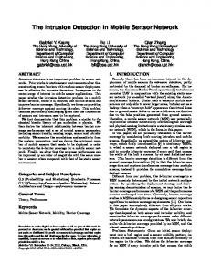
In this section, we focus on the case where the cats have a longer sensing range than the mouse. In this case, the mouse is always detected before it can see the cat; hence, the mouse can be considered a “blind” mouse. A. Strategy of the mouse Since a blind mouse cannot sense a cat’s actual movement, the mouse is assumed to have some high level information about the cats’ movements in order to avoid detection. Specifically, we assume that the mouse knows the statistical movement model and the sensing range Rc of the cats. Based on the information, we estimate the probability of finding at least one cat for any position in the network, and design the best strategy for the mouse accordingly. With a sensing range Rc , each cat controls a circular region of area πRc2 . Roughly speaking, each cat controls a square region—which we call a cell—of size s × s, √ with s = πRc . We then consider the network area to consist of X/s by Y /s disjoint cells, with each cat controlling the cell in which it is currently located. The presence matrix Π is defined such that Π[x, y] denotes the probability that at least one cat is present in cell i = (x, y) at any instant (when the context is clear, we use πi as a shorthand for Π[x, y]); note that Π can be obtained since the cats’ movement model is known. For instance, Figure 1 shows the presence matrix for a single cat (i.e., Nc = 1) moving under the random waypoint (RWP) algorithm [2] in a network area of 10 × 10 cells. 0.02 0.018 0.016 0.014 0.012 Probability
0.01 0.008 0.006 0.004 10
0.002 7
0 1
2
3 X
4 4
5
6
7
8
9
Y
1 10
Fig. 1. The presence matrix with 10 × 10 cells for a single cat moving under the RWP algorithm in the network area. The mean of the probabilities is 0.01, while the standard deviation is 0.012.
Remark: If Nc > 1 and the cats are moving independently under the same movement model, it is easy to obtain the presence matrix Π for Nc cats based on the presence matrix of a single cat. In particular, let pi be the presence probability of one cat in cell i. Then, the presence probability for at least one of the Nc cats appearing in cell i isPπi = 1 − (1 − pi )Nc . Also note that P and i πi ≤ Nc . i pi = 1
Dynamic programming solution for the best strategy: Given the presence matrix Π, what strategy should the mouse use to maximize the expected detection time? One simple greedy strategy is for the mouse to continually move to the neighboring cell having the lowest presence probability, and stop moving when all the current cell’s neighbors are more dangerous (i.e., they have a higher presence probability). The intuition is that the expected detection time will immediately increase whenever the mouse visits a new cell along the path. However, the greedy strategy may not always find the best path for the mouse, since it prevents the mouse from considering those paths that temporarily access a more dangerous neighboring cell but will eventually lead to a safe network location. For example, in Figure 2, the greedy strategy suggests that the mouse should move from cell a to cell c along the illustrated path, and finally stop at c. However, under most values of the mouse’s and cat’s speeds, the optimal path for the mouse is to move from cell a to cell b. 0.0005
0.0005
0.0005
0.0075
0.0075
0.0075
0.0075
0.0005
0.0075
0.03
0.03
0.03
0.03
0.03
0.03
0.0075
0.0075
0.03
0.021
0.023
0.025
0.03
0.0075
0.02
b
a 0.0075
0.03
0.018
0.03
0.03
0.03
0.03
0.0075
0.0075
0.03
0.03
0.016
0.014
0.01
0.03
0.0075
"hill" of high probability optimal escape path local greedy escape path
c 0.0075
0.03
0.03
0.03
0.03
0.03
0.03
0.0075
0.0075
0.0075
0.0075
0.0075
0.0075
0.0075
0.0075
0.0075
Fig. 2.
A greedy movement strategy may not be optimal.
To avoid missing the optimal path, we apply the dynamic program as shown in Figure 3. In the figure, there are three groups of variables, namely E[Tidetect ], move E[Tistay ], and E[Tk,i ]. The value E[Tidetect ] represents the expected detection time when the mouse starts at cell i and uses the best path among the paths considered so far. This value will be updated as the algorithm proceeds, and will eventually hold the desired expected detection time when the mouse uses the best path among all possible paths. The value E[Tistay ] denotes the expected detection time when the mouse starts at cell i and stays there forever. Finally, the value move E[Tk,i ] denotes the expected detection time when the mouse starts at cell k, moves to a neighbor cell i, and follows the best strategy once it reaches cell i. In the algorithm, we initialize E[Tidetect ] to E[Tistay ] for each cell i in Line 1, and insert the cell into a heap with key value E[Tidetect ], sorted in decreasing order (Line 2). For each iteration (Lines 3-12), we first extract the cell i with the largest key value from the heap, so that the value E[Tidetect ] will not be further updated. Then,
M AXIMIZE D ETECT T IME() 1 Initialize E[Tidetect ] of each cell i with E[Tistay ] 2 Put each cell i into a max-heap using E[Tidetect ] as key 3 while heap is not empty 4 Extract cell i from heap with largest key 5 for each neighbor cell k of i move ] 6 Calculate E[Tk,i move ] > E[T detect ] 7 if E[Tk,i k move ] 8 Update cell k’s key E[Tkdetect ] to E[Tk,i 9 Re-insert cell k into the max-heap 10 Mark i as k’s next step 11 end if 12 end for 13 end while Fig. 3.
Z
ℓ=0
tk,i
It can be shown that the dynamic program has time complexity O(n log n), where n = XY /s2 . We omit the analysis due to limited space.
for each neighboring cell k of i, we update E[Tkdetect ] move to E[Tk,i ] if the latter value is larger, meaning that the mouse starting at cell k can benefit from moving to cell i. If there was an update, we reinsert cell k into the max-heap with the updated key value (Lines 5-8). Also, we mark cell i to be the next cell to move to when the mouse is in cell k (Line 9). The correctness of the algorithm follows from the fact that when cell i is removed from the heap in Line 3, E[Tidetect ] is set to the expected detection time for a mouse starting at cell i and using the best path. This is because all the paths that go through a neighbor cell k of cell i either (i) are already considered if cell k is removed from the heap before cell i, or (ii) yield a smaller expected detection time if cell k is still in the heap. It remains to show how to compute E[Tistay ] and move ]. To do so, we introduce a concept called the E[Tk,i cell sojourn time, which is the length of time that a cat stays in the current cell before it moves to a neighboring cell. The expected sojourn time, denoted by E[T s ], can be calculated since the cats’ movement model is known. For the purpose of estimation, we may assume that the status of whether any cat is present in a certain cell is unchanged during the time interval [ℓt, (ℓ + 1)t), for t = E[T s ] and any non-negative integer ℓ. Then, we can estimate E[Tistay ] by (ℓE[T s ])πi (1 − πi )ℓ = E[T s ]/πi .
t
πi (1 − πi ) E[T s ] tdt + (1 − πi ) E[T s ] (E[Tidetect ] + tk,i )
0
Dynamic program for the mouse’s best strategy.
∞ X
tk,i
(1)
move ] based on the optimal To calculate E[Tk,i detect E[Ti ], we let tk,i be the time taken by the mouse to move from (the center of) cell k to (the boundary of) cell i. Then, the mouse will either be caught in cell k, or it can reach cell i so that it is expected to be caught after another time of E[Tidetect ]. The probability that it can reach cell i without being caught can be estimated by s (1 − πi )tk,i /E[T ] . Using an approach similar to the one move used to estimate E[Tistay ], we can estimate E[Tk,i ] by
B. Strategy of the cats Based on the strategy in the previous section, the mouse may eventually move to a safer position that has a lower cat presence probability than its current position, thereby maximizing the expected detection time. Accordingly, the best strategy for the cats is to maximize the minimum presence probability among all the cells in Π. The maximin strategy implies that when the cats are moving independently under the same movement model, the best choice for each cat is to move in a way such that the presence probability is the same in each cell. (We call the resulting presence matrix in which all the entries have equal values a uniform presence matrix.) With a uniform presence matrix, there is no particularly safe place for the mouse to stay, which reduces the (worstcase) expected detection time of the mouse. One simple example movement that will yield a uniform presence matrix is to sequentially and circularly scan all the network cells. However, the deterministic nature of the cats’ movements may allow the mouse to accurately predict where the cats will be and therefore easily avoid them. Hence, a probabilistic movement strategy for the cats is necessary and preferred in practice. In Section V-B, we will present a simple, practical, and randomized movement model which can achieve a presence matrix close to being uniform. If Nc cats move in disjoint areas of the network, the sum of πi in the presence matrix is equal to Nc , which is greater than the sum of πi if the cats move independently to monitor the network area. This suggests that if the cats are allowed to move in a coordinated way, we should always assign them disjoint areas in the network to monitor. Accordingly, the best strategy for the cats is to divide the network into Nc equally sized partitions, in which one cat moves within each partition to yield a uniform presence matrix. V. The Seeing Mouse: Rc < Rm In this section, we discuss the case when the mouse has a larger sensing range than the cats. In this case, once a cat enters the mouse’s sensing range, the mouse can know the cat’s movement in advance without being detected. We first propose a strategy for the mouse to escape from the cats based on such advance knowledge. We then discuss some possible strategies that the cat may use to reduce the detection time, knowing that the mouse may run away when it sees the cat.
γ is maximized when this angle is π/2
A. Strategy of the mouse We first study the special case in which there is only one cat in the network. Then, we generalize the strategy to the case of multiple cats. Avoiding a single cat: When the mouse tries to escape from a cat, it is better if it can move in a direction β such that the minimum distance between the mouse and the cat (assuming that the cat does not change its speed and moving direction) in the future is as large as possible. Let C and M be the current positions of the cat and the mouse, respectively. Let α be the moving direction of the cat. Then, the position of the cat at time t, denoted by C(t), can be expressed as C + (Vc cos α · ˆı + Vc sin α · ˆ) t.
(2)
Similarly, if the mouse chooses to move in a direction β at a speed of Vm , the position of the mouse at time t, denoted by M (β, t), can be expressed as M + (Vm cos β · ˆı + Vm sin β · ˆ) t.
(3)
Then, the distance between the cat and the mouse at time t is equal to d(β, t) = kC(t) − M (β, t)k. By differentiating d(β, t) with respect to t, we can find the minimum distance between the mouse and the cat for t ≥ 0. We denote such a distance by d∗ (β). In other words, in order to maximize the distance from the cat in the future, the mouse should find a direction β ∗ such that β ∗ = argmax d∗ (β). (4) β
Remark: In fact, by a simple geometric argument, the optimal β ∗ for the single-cat case can be easily obtained. Essentially, the cat is moving in a vector V~c = Vc cos α · ˆı + Vc sin α · ˆ, while the mouse choosing a direction β is moving in a vector V~m = Vm cos β · ˆı + Vm sin β · ˆ. Equivalently, we may assume that the cat is stationary, ~ = V~m − V~c while the mouse is moving in a direction V towards the cat. To maximize the distance between the cat and the mouse, we want (the absolute value of) the ~ and the vector from the mouse to the angle γ between V ~ −M ~ ) to be as large as possible. As shown cat (i.e., C in Fig. 4, we have � � Vm . (5) β ∗ = α + arccos Vc Avoiding multiple cats: We have shown how the mouse can choose the optimal direction β ∗ when there is only one cat. In the case of multiple cats, we need to find a β ∗ that maximizes the minimum distance to all the cats in the future. Using similar notations, we let d∗i (β) denote the minimum distance between the mouse and the ith cat in the future, assuming that the mouse is moving in
Mouse V Vm -Vc
to maximize γ
Mouse Vm
γ
β*
γ
-Vc
Vc α
Cat
β *=α+arccosVm
Vc
Vc
α
Cat
~ = V~m − V~c (a) V
(b) To maximize γ.
The mouse’s choice of β ∗ to maximize γ.
Fig. 4.
the direction β. In other words, if there are j cats within the sensing range of the mouse, we have n o β ∗ = argmax min d∗1 (β), d∗2 (β), . . . , d∗j (β) . (6) β
Notice that in the case of multiple cats, a direction β that maximizes the minimum distance for one cat does not necessarily yield a short minimum distance for another cat. Finding the optimal β ∗ may require us to consider all the Ω(j 2 ) intersections between any two of the j curves d∗i (β). An alternative way is to obtain a close estimation of β ∗ , by choosing a small angle δ and computing all d∗i (β) values for β = 0, δ, 2δ, 3δ, . . . , ⌊2π/δ⌋δ, and then finding β ∗ based on only these values. The drawback of the above estimation is that we may miss the optimal β ∗ when it is not a multiple of δ. However, there are only O(j/δ) values to compute, and the simplicity of the method will usually allow us to obtain a good enough β ∗ efficiently in practice. Degree of freedom and a revised strategy: In general, it is not necessary for the mouse to choose the optimal direction β ∗ to avoid being caught. It is because when choosing a direction β, a mouse will not be detected as long as its minimum distance to all the cats in the future is larger than the cats’ sensing range Rc . Hence, the mouse may choose a direction from a feasible set B such that � � ∗ (7) B = β min {di (β)} > Rc . 1≤i≤j
Thus, the larger the size of B is, the more directions the mouse can choose from, so that it is more likely for a mouse to escape successfully. Note that the mouse may have fewer choices when it is located at the boundaries or the corners of the network area. In fact, if the cats move under the RWP algorithm and the mouse uses the above strategy to escape (so that it chooses to move at an angle of β ∗ when one or more cats are around, and stops moving when no cat is around), the results in Fig. 5 show that the mouse will likely be “pushed” to the corners/boundaries of the network, and then be caught there.
0.018 0.016 0.014 0.012 0.01 Probability 0.008 0.006 0.004 9
Fig. 5. The black dots show the positions where the mouse is detected in 50,000 simulation runs. The mouse is caught at the the network corners and boundaries in most cases.
0.002
7 5
0 1
2
3 3
4
5
6
X
This leads to a revised strategy for the mouse to always move towards the center region of the network whenever there is no cat detected within its sensing range. We call this the centric strategy. Our results in Section VI show that this strategy always works well among the strategies evaluated, even if the cats use RWP movement. B. Strategy of the cats Since a cat knows that the mouse may see it before it sees the mouse, the cat may assume that the mouse will try to run away from it in advance. One logical choice of strategy for the cats is then to visit more frequently the center region of the network, where the mouse has more freedom to move and escape. As shown in Figure 1, a cat can achieve the goal of visiting the center region more often by playing the RWP strategy. On the other hand, the cats may also benefit from a movement strategy that will yield a uniform presence matrix, so that they will eliminate safe havens for the mouse to hide in. As both kinds of strategy have their merits, we will compare their empirical performance in Section VI. We now describe a simple and practical realization of random movement that will allow the cats to achieve a close approximation to the uniform presence matrix. In the movement algorithm, a cat moves in a straight line until it hits the boundary or a corner of the network area. Whenever it reaches the boundary/corner, it selects a direction randomly and uniformly from all the feasible directions and proceeds to move in the selected direction. We call this movement model the bouncing strategy. Figure 6 shows the presence matrix for a cat moving under the bouncing model. VI. Experimental Results A. The blind mouse: Rc ≥ Rm
This section evaluates the case of a blind mouse. Unless otherwise specified, we report average results over 100 simulation runs, each lasting 200,000 seconds. We omit the standard deviations, because they are very small compared with the means. In the discussion, when a node deterministically cycles through all the cells in
Y
7
8
1 9
10
Fig. 6. The presence matrix with 10×10 cells for a single cat moving under the bouncing strategy in the network area. The matrix is close to the uniform presence matrix.
the network area, we will refer to the movement as the scan strategy. 1) Benefits of dynamic programming solution for the mouse: We compare the performance of different movement strategies for the mouse in Table I. In the table, the column “DP” refers to the case when the mouse determines its movement by the dynamic programming strategy in Section IV-A. The mouse is initially located at the center of the network area. The column labeled “Stay” in Table I is used for baseline comparison, and refers the to case when the mouse simply stays at its starting position (i.e., it does not move at all afterwards). The experiments use one cat. Its movement strategy is shown as the rows of Table I, and is chosen to be (1) the uniform scan strategy, (2) the bouncing strategy in Section V-B, and (3) the random waypoint (RWP) strategy, in three sets of runs. From the table, notice that the mouse can achieve a significantly higher average detection time by playing the dynamic programming strategy, as the analysis in Section IV-A shows. TABLE I AVERAGE DETECTION TIME ( IN S ) FOR DIFFERENT CAT AND MOUSE MOVEMENT STRATEGIES IN A 500 M BY 500 M NETWORK . Vc = Vm = 10 M / S , Rc = 25 M , AND THE MOUSE IS INITIALLY LOCATED AT THE CENTER OF THE NETWORK . Mc \ Mm uniform scan Bouncing RWP
DP 1083.26 628.66 2823.26
RWP 415.31 442.23 271.73
Stay 511.50 305.03 226.13
2) Uniform presence matrix benefits the cat: The “DP” column in Table I also shows how a uniform presence matrix may benefit the cat. From the results, notice that the simple scan strategy can greatly reduce the detection time compared with the non-uniform RWP strategy. However, as discussed in Section IV-B, the deterministic nature of the scan strategy may allow the mouse to predict where the cat will be in advance and thus effectively avoid the cat. To avoid the problem, the
Average detection time (s)
60000
RWP Bouncing
50000
3000 2500 2000 1500 1000 500 0 0
40000
0 20
30000
40
50
60
20000
80 100
10000
100
Vm (m/s)
Vc (m/s)
0 0
10
20
30 Rc (m)
40
50
60
Fig. 7. Average detection time (in s) of the mouse versus the cat’s sensing range Rc (in m); Vc = Vm = 10 m/s.
4) Number of cats: In this experiment, we measure the average detection times when the number of cats is varied. The network area is 500 m × 500 m, and the sensing range of each cat is 25 m. Similar to the previous experiment, the mouse plays the dynamic programming strategy, while the cats independently play either the RWP or the bouncing strategy. Fig. 8 shows that as the number of cats increases, the average detection time decreases, approximately like inversely proportional to Nck , where k is a constant slightly larger than one. 3000 Average detection time (s)
mouse moves at a higher speed. This is because a faster mouse can move from its current position to a safe position more quickly, and benefit from staying in the safe position longer. We also find that the mouse can benefit more from moving at a higher speed, if the cat itself is moving at a higher speed. This shows that a fast cat will force the mouse to be fast to avoid detection.
Average detection time (s)
bouncing strategy can closely approximate the uniform presence matrix without being deterministic. 3) Effects of the cat’s sensing range: In this experiment, there are one cat and one mouse moving in a 500 m × 500 m network area. The mouse plays the dynamic programming strategy. The cat uses (1) the RWP strategy and (2) the bouncing strategy, in two different runs. We measure the average detection time of the mouse for different sensing ranges, Rc , of the cat. Fig. 7 shows that as Rc increases, the average detection time decreases as an inversely proportional function of Rc , showing that the cat’s ability to detect the mouse increases proportionally to its sensing capability.
RWP Bouncing
2500 2000 1500 1000 500 0 0
10
20
30
40
50
Nc
Fig. 8. Average detection time (in s) versus the number of cats Nc in a 500 m by 500 m network area; Vc = Vm = 10 m/s.
5) Effects of Vc and Vm on dynamic programming solution: In this experiment, there are one cat and one mouse. We illustrate how the expected detection time of the mouse varies with different speeds Vc and Vm of the cat and the mouse, respectively. The mouse plays the dynamic programming strategy. Fig. 9 shows that the average detection time is reduced when the cat moves faster (i.e., Vc is higher). This is because a faster cat can cover a larger area in the same amount of time. Notice also that the detection time increases when the
Fig. 9. Average detection time (in s) versus the speeds (in m/s) of the cat and the mouse in a 500 m by 500 m network. Rc of the cat is 15 m.
We further show that the path of movement computed by the dynamic program in Figure 3 is dependent on the speed of the mouse. In Figures 10(a) and 10(b), the gray level represents the cat’s presence probability (the darker an area, the lower the cat’s presence probability in the area). The cat has a speed of 10 m/s. The arrows in the figure show the escape paths of the mouse in a 500 m × 500 m network area divided into 10 × 10 cells. The paths when the mouse has a speed of 10 m/s are shown in Figure 10(a). The paths when the mouse has a higher speed of 15 m/s are shown in Figure 10(b). In the figure, cells j and k are cell i’s neighbor. Cell k is safer than j, and both of them are safer than i. Assume that the mouse is currently in cell i. Notice that when the mouse has the lower speed, it will move to the less safe neighbor j because j is closer in distance than k. Choosing the closer neighbor allows the mouse to leave the more dangerous cell i soon (considering that the mouse moves slowly). When the mouse has the higher speed, it can afford to move a longer distance before leaving cell i. Hence, it will choose to move directly to the safer neighbor k although k is farther away. B. The seeing mouse: Rm > Rc We now evaluate the case of a seeing mouse. In the experiments, unless otherwised specified, the cats play the bouncing strategy and Rc = 5 m and Rm = 10 m. We report maximum, minimum, and average results over 5,000 simulation runs within a 100 m by 100 m area. 1) Movement direction β for the mouse: In this experiment, we report the optimal direction β ∗ calculated
1
i j k
Fraction of feasible solutions
0.9
i j k
0.8 0.7 Maximum
0.6 Median 0.5 0.4
Maximum
0.3
Mean
Mean 0.2
Median
0
0.0115
0.0200
0.0030
(a) Vc = Vm = 10 m/s.
0.0115
0.0200
Fig. 10. Escape paths calculated by the algorithm MaximizeDetectTime() for a 500 m by 500 m network area divided into 10 by 10 grids, for different speeds of the mouse.
by Eqn. 6 to maximize the minimum distance between the cats and the mouse. We use Vc = Vm = 5 m/s. There are six cats and one mouse. Figure 11, shows the minimum distance of the mouse from each cat, as a function of the mouse’s direction of movement β. In the figure, the thick line shows the minimum distance of the mouse from any of the cats. Of the thick line, the dark segment shows the range of the movement angles over which the minimum distance (from any of the cats) is maximized, and thus gives the range of the optimal maximin solutions computed. Any angle that falls within the range can be used by the mouse as its optimal movement direction. Minimum distance between cat and mouse (m)
90 Cat 1 Cat 2 Cat 3 Cat 4 Cat 5 Cat 6 Minimum Maximin
80 70 60 50 40 Range of maximin solutions 30
Minimum distance to all the cats 20 10 0
0
50
100
0
10
20 30 Sensing range (m)
40
50
(b) Vc = 10 m/s, Vm = 15 m/s.
150 200 Beta (degree)
250
300
350
Fig. 11. The minimum distance d∗ (β) calculated by Equation 6 between six cats and one mouse as a function of the mouse’s movement direction β. The cats and the mouse are initially randomly placed in a 100 m by 100 m network.
2) Effects of Rc and Nc : In this experiment, we use ten cats, and show how Rc can affect the range of maximin solutions available to the mouse as it tries to find an optimal angle of movement. In Figure 12, we report the fraction of the movement angles that are in the feasible set B (defined by Equation 7) as a function of Rc . The results show that the fraction of feasible solutions decreases like exponentially as Rc increases (up to Rm ), showing that the mouse’s degree of freedom in choosing a solution is severely restricted as the cat’s sensing capability increases. We next consider the effects of Nc , the number of cats. In Figures 13 and 14(a), we show that as Nc increases,
Fig. 12. The fraction of feasible solutions calculated by Equation 7 as a function of the cat’s sensing range Rc . Ten cats are randomly placed in a 100 m by 100 m network. Rm = ∞.
both the optimal minimum distance (of the mouse) from any of the cats and the average detection time decrease. 140 Maximum Mean Median Minimum
120 Maximin distance to any cats (m)
0.0030
Minimum
Minimum
0.1
100 80 60 40 Minimum
20 0
0
20
40 60 Number of cats
80
100
Fig. 13. Statistics of the maximin distance of the mouse from any of the cats, as a function of the number of cats Nc . Both the cats and the mouse move according to the bouncing strategy in a 100 m by 100 m network area.
3) Effects of Rm and Vm : We show the impact of the mouse’s sensing range Rm on the detection time in Figure 14(b). As Rm increases, the mouse can detect the cats earlier and are better able to make the necessary moves to avoid the cats. Hence, the detection time increases significantly at first. As Rm increases beyond 9 m, however, the detection time does not change much. This shows that information about the cats that are far away (as captured by a large sensing range Rm ) may not be that useful to the mouse in determining its immediate course of action. The results in Figure 14(c) show that the detection time generally increases as the mouse’s speed increases. This is because a faster mouse can avoid the cats more quickly and allow itself more choices of the optimal movement direction β ∗ . 4) Comparison of different strategies: We discussed the bouncing and centric strategies for the mouse in Section V-A and Section V-B, respectively. In the seeing mouse case, these strategies define what the mouse should do when it sees no cat within its sensing range. An alternative strategy in such a situation is for the mouse to simply stay where it is, presumably to
4500
2000 Mean Median Minimum Maximum
3000
Detection time (s)
Detection time (s)
3500
2500 2000 1500
Maximum
Mean
Mean
1600
Median
2000
1400
Minimum
Median Minimum
1200 1000 800
1500
1000
600
1000
400
500
Minimum
500 0
2500 Maximum
1800
Detection time (s)
4000
Minimum
Minimum 200
0
5
10 Number of cats
15
20
0
0
2
4
6 8 10 12 Mouse sensing range (m)
(a)
14
16
18
0
0
5
10 Mouse speed (m/s)
(b)
15
20
(c)
Fig. 14. Statistics of the detection times as a function of (a) Nc , (b) Rm , and (c) Vm . The cats randomly move in a 100 m by 100 m network. Both the cats and the mouse use the bouncing strategy.
RWP Mc Bouncing Stay
Static
Centric
1600 1400 1200 1000 800 600 400 200 0 Bouncing
Average detection time (s)
conserve energy, and we call it the static strategy. In this experiment, we compare the performance of these strategies for the mouse, while ten cats in the network play either the bouncing or the RWP strategy. The average detection time results are shown in Fig. 15. As a baseline case for comparison, we also show a “stay” strategy in which the mouse simply stays at its starting position; i.e., the mouse never moves (i.e., Vm = 0) and does not apply Equation 6 to determine its angle of movement. From Fig. 15, notice that bouncing is the best strategy for the cats, where their presence matrix is approximately uniform. For the mouse, its best strategy depends on the cats’ strategy. When the cats play the bouncing strategy, the best strategy for the mouse is centric. When the cats play the RWP strategy, the best strategy for the mouse is bouncing. The results show an interesting interplay between the cats’ and the mouse’s movements. When the cats use the bouncing strategy, the mouse benefits by moving towards the center of the network, where it has a higher degree of freedom as discussed in Section V-A. However, this higher degree of freedom is offset, in the case of this experiment, when the cats use the RWP strategy to achieve a higher presence in the center area. The static strategy performs the worst in all of the cases measured.
Mm
Fig. 15. Average of the mouse detection time (in s) under different strategies for the cats and the mouse in a 100 m by 100 m network. V c = 5 m/s, V m = 10 m/s, Rc = 5 m, and Rm = 10 m.
VII. Conclusions We have considered the cat-and-mouse game between an intelligent mobile target trying to evade detection and
a group of mobile sensors trying to detect the target as quickly as possible. For a blind mouse, we presented and analyzed a dynamic program for the mouse to maximize its expected detection time, assuming high level knowledge about the cats’ movements. We further argued that the cats’ choice of a uniform presence matrix can minimize the worst case (over the mouse’s starting positions) expected time to detect the mouse. For a seeing mouse, we presented an efficient optimal algorithm based on geometric arguments that allows the mouse to maximally delay detection by reacting to the cats’ movements within its sensing range. We then discussed possible counter strategies by the cats to reduce the expected detected time. Extensive experimental results verified that the optimal algorithms can significantly outperform alternative heuristic algorithms. R EFERENCES [1] N. Bisnik, A. Abouzeid, and V. Isler, “Stochastic event capture using mobile sensors subject to a quality metric,” in Proc. MOBICOM, September 2006. [2] J. Broch, D. A. Maltz, D. B. Johnson, Y. C. Hu, and J. Jetcheva, “A performance comparison of multi-hop wireless ad hoc network routing protocols,”, in Proc. MOBICOM, 1998. [3] H. Cao, E. Ertin, V. Kulathumani, M. Sridharan and A. Arora, ”Differential games in large-scale sensor-actuator networks,” in Proc. Int. Conf. Info. Proc. in Sensor Networks, 2006. [4] J. P. Hespanha, K. H. Jin, and S. Sastry, “Multiple-agent probabilistic pursuit-evasion games,” in Proc. IEEE Conf Decision and Control, vol. 3, 1999. [5] B. Liu, P. Brass, O. Dousse, P. Nain, and D. Towsley, “Mobility Improves Coverage of Sensor Networks,” in Proc. MobiHoc, 2005 [6] S. Meguerdichian, F. Koushanfar, G. Qu, and M. Potkonjak, “Exposure In Wireless Ad-hoc Sensor Networks,” in Proc. MOBICOM, 2001. [7] L. Schenato, S. Oh, and S. Sastry, “Swarm coordination for pursuit evasion games using sensor networks,” in Proc. Int. Conf. on Robotics and Automation, 2005. [8] R. Teo, J. S. Jang, and C. J. Tomlin, “Automated Multiple UAV Flight – the Stanford DragonFly UAV Program,” in Proc. IEEE Conf. Decision and Control, Dec 2004. [9] Z. Vincze, D. Vass, R. Vida, A. Vidacs, and A. Telcs, “Adaptive sink mobility in event-driven multi-hop wireless sensor networks,” in Proc. InterSense, 2006. [10] G. Wang, G. Cao, and T. L. Porta, “Movement-assisted sensor deployment,” in Proc. IEEE INFOCOM, 2004.