Jul 7, 1994 - LEE M. GARTH, STUDENT MEMBER, IEEE, AND H. VINCENT POOR, FELLOW, IEEE. 0018-9219/94$04.00 0 1994 IEEE. Invited Paper.
Detection of Non-Gaussian Signals: A Paradigm for Modern Statistical Signal Processing LEE M. GARTH, STUDENT MEMBER, IEEE, AND H. VINCENT POOR, FELLOW, IEEE Invited Paper
Non-Gaussian signals arise in a wide variety of applications, including sonar, digital communications, seismology, and radio astronomy. In this tutorial overview, a hierarchical approach to signal modeling and detector design for non-Gaussian signals is described. In addition to being of interest in applications, this problem serves as a paradigm within which most of the areas of active research in statistical signal processing arise. In particular, the methodologies of nonlinear signal processing, higher order statistical analysis, signal representations, and learning algorithms, all can be jutaposed quite naturally in this framework.
I. INTRODUCTION The purpose of this paper is to present a survey of techniques for the detection of non-Gaussian signals. NonGaussian signals arise in a wide variety of applications, including sonar, digital communications, seismology, and radio astronomy. The exploitation of non-Gaussian structure in detecting signals usually requires the use of much more sophisticated signal processing methodology than is needed for detection algorithms based on traditional Gaussian models. However, this additional complexity is usually rewarded with substantial gains in detection sensitivity. Thus as advances in signal processing technology have made it possible to implement such sophisticated processing, considerable interest in ways of exploiting nonGaussian structure has emerged. A related, but somewhat more mature, area of technology is that of signal detection in non-Gaussian noise. Although comprehensive reviews of this area have appeared in recent years (e.g., see [l]), no comparable general work exists for the detection of non-Gaussian signals. Thus the present paper is motivated in part as a remedy for this situation. However, this survey is also motivated in a larger context, in which the problem of detecting non-Gaussian signals can Manuscript received August 24, 1993; revised April 1, 1994. This work was supported by NOSC under Contract N66001-90-C-7004 under the Small Business Innovation Research Program, with Dr. C. Persons of NOSC as COTR and with funding from the Office of Naval Research. L. M. Garth is with Techno-Sciences, Inc., Urbana, IL 61801 USA. H. V. Poor is with the Department of Electrical Engineering, Princeton University, Princeton, NJ 08544 USA. IEEE Log Number 9401812.
be viewed as a unifying focal point for a general class of problems being addressed by much of the current research in statistical signal processing. In particular, many of the most active research areas in statistical signal processing-e.g., wavelet decompositions, neural networks, higher order spectral analysis-arise naturally in this problem. In this sense the problem of detecting non-Gaussian signals establishes a framework within which much of modem signal processing research can be discussed. Thus an exposition of this approach should be of interest to a broad spectrum of electrical engineers (in addition to specialists in the abovenoted applications). The purpose of this paper is, therefore, to organize and survey the methodology in this area, and to present it in a unified form. The general organization of the paper is to adopt a hierarchical framework within which the non-Gaussian signal detection problem can be cast. This hierarchy begins with a consideration of parametrically determined signals; and ranges through stochastic signals, both fully and incompletely modeled and finally to unstructured signals. Naturally, in this progression the degree to which optimum procedures can be designed and analyzed lessens as the signals become less structured. Thus at the highest level of modeling the methodology is centered on the use of optimum procedures and their performance characteristics; whereas, these things become less tractable for the stochastic signals. And finally, the focus tums to largely algorithmic issues for the unstructured signals. The paper is organized as follows. In Section 11, we present some general background and discuss briefly the hierarchy of models to be explored. Then, in Sections 111-VI, the various levels of the hierarchy are considered separately and in detail. Section VI1 includes a summary as well as some concluding remarks. 11. A HIERARCHY OF MODELS Throughout most of this paper, we will consider the basic problem of detecting the presence or absence of a signal {St;0 5 t 5 T } in a set of measurements 0 5 t 5 T},
{x;
0018-9219/94$04.00 0 1994 IEEE PROCEEDINGS OF THE IEEE, VOL. 82, NO. 7, JULY 1994
1061
Authorized licensed use limited to: UNIVERSITY OF WINDSOR. Downloaded on February 25,2010 at 19:25:51 EST from IEEE Xplore. Restrictions apply.
corrupted by independent additive, white Gaussian noise (AWGN). This problem can be described mathematically in terms of a hypothesis test between the following pair of statistical hypotheses:
Ho:Yt=Nt,
OltlT
versus
where { N t ; O 5 t 5 T} is the aforementioned AWGN process. Two crucial simplifying assumptions are being made here; namely, that the noise is white and Gaussian, and that it is independent of the signal. Although both of these assumptions are often violated in applications, they are invoked here in order to focus attention on the effects of the signal model in detector design. The effects of signal and noise dependence, and of non-Gaussian noise are discussed briefly in Section IV. We also assume for simplicity (and without loss of generality) that the noise has unit spectral height, so that the signal energy can be taken to be the signal-to-noise ratio. In the most generally accepted sense of optimality, optimum decisions in the model ( 1 ) involve thresholdcomparison tests based on the likelihood ratio between the two hypotheses. This ratio is a functional mapping the observed waveform to the positive numbers, and is given by
L ( Y z )= E ( exp
(LT
StYt dt -
f I T S , "dt) }
(2)
where E { . } denotes expectation taken over the signal statistics. When possible, the goal in detection system design should be to emulate the behavior of such a likelihood ratio test; and in the sequel, we will discuss the structure of the likelihood ratio under several signal modeling assumptions of interest. However, it is not always possible to specify the statistics of the signal to the degree required to form the likelihood ratio. Thus there are many alternative techniques for detection in this problem, depending on the level of modeling detail available to the designer. Such models and the detection systems arising therefrom are included in our discussion. As noted in the Introduction, the thrust of this work is to detail a hierarchy of models for signal statistics and the corresponding implications for detection system implementation, analysis, and complexity. This hierarchy proceeds from one extreme of a signal with completely known structure, through a number of levels of modeling detail, to the opposite extreme of a signal with completely unknown structure. This hierarchy can be envisioned as a set of four general strata, each of which contains several levels of modeling detail. These four strata are, in order of decreasing model detail: parametrized signals, fully modeled stochastic signals, partially modeled stochastic signals, and unstructured signals. Within the first of these four categories, there are completely known signals, for which the optimum detection 1062
system is the classical matched-filter detector; and parametrized signals that can be detected optimally via parallel banks of matched filter detectors or by adaptive matched filter detectors. In the second stratum, there is a rich variety of models, and a correspondingly broad class of optimum detection systems, all of which involve (often complex) nonlinear processing of the observed waveform. The third of these four strata includes models based only on secondand higher order moment descriptions of the signal. This level of description is insufficient to specify the likelihood ratio, and suboptimal techniques are therefore used. The last of these four categories includes the situation in which no signal structure is known, and detector design must be based exclusively on empirical data, or on nonparametric methods. Thus the underlying philosophy at this stratum is one of pattern recognition. We now proceed, in the following sections, to detail this hierarchy. 111. PARAMEnUZED SIGNALS The first level of detail includes signals that are completely known except possibly for a small set of unknown parameters. It should be noted that this type of model is appropriate for applications such as digital communications and radar, but is less so for applications such as passive sonar or seismology. However, this level of modeling and design is of interest in any application as a benchmark with which more practical signal models and detection systems can be compared. A . Deterministic Signals The simplest case in a statistical sense and the highest possible level of structure is the description of { St;0 5 t 5 T } as a deterministic signal. For this case, the observer is assumed to have an exact knowledge of the signal. Due to the delays and distortion introduced by many channels, this model is often not realistic, and systems designed under this model can have inferior performance to those designed to take into account these phenomena. However, due to the simple design and exact performance analysis of the matched filter detector that results from this model, many operative detection systems are based on this model to some degree. As mentioned above, we consider the well-known deterministic signal model and analyze the performance of the matched filter detector here to establish benchmarks with which less structured models can be compared. ModellDetection System: In this case, the statistical hypothesis test of (1) can be written as
versus
where { st; 0 I t I T} is a deterministic signal. In order to make this model meaningful, it is assumed that the signal PROCEEDINGS OF THE IEEE. VOL. 82, NO. 7, JULY 1994
Authorized licensed use limited to: UNIVERSITY OF WINDSOR. Downloaded on February 25,2010 at 19:25:51 EST from IEEE Xplore. Restrictions apply.
k'
Fig. 1. Continuous-time matched filter detector.
Fig. 2. Discrete-time correlation (matched filter) detector.
energy is finite, i.e.,
versus
Hi : Y , = N k Since { s t ; O is simply
5 t 5 T} is
known, the likelihood ratio (2)
[Jo
L Jo
(This is the so-called Cameron-Martin formula, a direct derivation of which can be found in [2].) Therefore, the optimum detection rule reduces straightforwardly to
6(Y,T)=
{::
Sk,
k = 1 , . . . ,72
where S k and N k correspond to samples of the signal and noise processes, respectively, and the samples { f v k ; k = 1,. . . , n} are assumed to be independent unit Gaussian random variables. It is well known that such a hypothesis test leads to an optimal detection system in the form of a correlation detector as shown in Fig. 2, where T is the detection threshold. This system is of course also a linear filter and is of complexity O ( n ) . The performance of this system is identical to its continuous-time counterpart, with the substitution n
2
if s , ' s t y t dt
-k
d2 = T sE. Y '.
r
k=l
70) satisfying Po(r8) = Q is independent of 8 for all 0 E A. In this case, the decision rule is formed by implementing the inequality implied by this (&invariant) critical region. Alternatively, when a UMP test does not exist, one can turn to the ML test, which consists of comparing the statistic
+ $),
-
f
a sin (w,t
a2 sin2 (w,t
I
.
On defining
Y, =
I
T
acos (wct)Y, dt
and
1 T
Y, =
a sin (wct)yt dt,
the likelihood ratio can be shown straightforwardly to be
s
aZT
e - 4 L ~ ( Y F ) de ~ (=~)21r
.
I'"
exp {Ycsin 8
+ Y, cos e } d6
aZT
= e-?I,(R)
where R = [Y,"+Y:]1/2 and IOis the zeroth-order modified Bessel function of the first kind. Since l o is a monotonic I064
PROCEEDINGS OF THE IEEE, VOL. 82, NO. 7, JULY 1994
Authorized licensed use limited to: UNIVERSITY OF WINDSOR. Downloaded on February 25,2010 at 19:25:51 EST from IEEE Xplore. Restrictions apply.
Fig. 5. Optimal noncoherent detector.
Fig. 6. Matched filter detector for sinusoid with unknown frequency.
function, the ratio-threshold test can be written
2 S(YT)=
ifR
7'
k IG1(e$T)
< where T is the appropriate threshold. This decision rule is implemented as the familiar noncoherent detector (i.e., the envelope detector) shown in Fig. 5. If, on the other hand, the amplitude of { s t ;0 5 t 5 T } is unknown but positive, the hypothesis test of (5) can be rewritten as
Ho:Yt=Nt,
05tlT
It should be noted that combinations of the above detection structures can be implemented; e.g., Doppler banks of noncoherent detectors are optimum for sinusoids of unknown frequency with uniformly distributed phase, etc. Performance Analysis: For a general signal of the form {st(B);O 0, where * denotes the conjugate transpose operation. The resulting generalized likelihood ratio test (GLRT) compares
+ +
=W
T W
with separating surface defined to be {z E Rd : tuT+(%) = 0). As shown by Cover [143], 4(z) can be defined so that the separating surface between two classes is a hypersphere or hypercone. The generalized form can approximate any arbitrarily complex decision surface if +(z)is made of high enough dimension and complexity. Unfortunately, along with this high dimension and complexity comes what is known as the “curse of dimensionality.” This problem is illustrated by the result that for quadratic discriminant functions of the form g(z) = (z- zo)*Q(z- zo), we have to solve for (d l)(d 2)/2 unknowns. Thus generalized linear discriminant functions are computationally expensive for an arbitrarily large number of features. Also, we need as many samples in the training set as there are degrees of freedom in the parametric function. We now restrict ourselves to linear homogeneous discriminant functions of the form g(z) = w T z .A data set is said to be linearly separable if basically the two classes can be separated using a hyperplane. A related result due to Cover [ 1431 is that the separating capacity of a hyperplane is two pattems per feature or dimension of zor degrees of freedom of w. A set of samples is separable but under-determines the discriminant function if the number of samples is less than twice the number of degrees of freedom. Since the system is under-determined, it is prone to instability. For a training set containing more samples than twice the number of features, the separating surface is over-determined and not necessarily linearly separable. However, the surface is stable in this case in the least squares sense [143]. Given these properties of discriminant functions and separating surfaces, the optimal coefficient vector w in some sense needs to be determined. Several methods have been developed to solve for w, some using iterative techniques and others performing batch calculations. For a linearly separable training set, the adaptive algorithm called the perceptron has been developed (more will be said about perceptrons in the section on neural networks). The perceptron has the following behavior, when wk denotes the kth updated version of the coefficient vector. (The coefficient vector is modified so that all of the samples for one class times -1 and for the other class times +1 lie on the same side of a homogeneous hyperplane. This is possible due to the linear separability of the set.) The algorithm cycles through the training set and updates the coefficient vector
+
wk+l
and the respective decision rule is
S(z)=
A broader class of discriminant functions is described by the generalized linear discriminant function
+
{I:+
> if w z z , za,
0
I
until the coefficient vector converges. Nilsson [ 1441 has demonstrated that this algorithm converges in a finite number of iterations. However, for the discriminant function to be over-constrained and stable, the training samples most likely will not be linearly separable. If this is the case, PROCEEDINGS OF THE IEEE, VOL. 82, NO. 7, JULY 1994
Authorized licensed use limited to: UNIVERSITY OF WINDSOR. Downloaded on February 25,2010 at 19:25:51 EST from IEEE Xplore. Restrictions apply.
the algorithm does not converge. A modification of the perceptron for nonseparable sets that converges by making use of a decreasing step size is described in [81]. This convergence problem with the perceptron has led researchers to use the least mean-squared error (LMSE) algorithm. Since the goal, as stated for the perceptron, is to find a coefficient vector w so that wTzi is approximately greater than 0 for all the zi’s, a coefficient vector w that satisfies wTz; z 1 , V i will provide this approximate .-z,ITand solution. If we define the matrix X = [zl. vector U = [l. . . 1IT, this later problem can be solved by minimizing the cost function (77) Solving V w J s ( w )= 0, we find that w* = Xtu, where Xt = (XTX)-lXTis the pseudo-inverse of X. If XTX is singular, we can express ~t using a singular value decomposition. The cost function (77) can also be minimized efficiently using the recursive Widrow-Hopf gradient algorithm to solve for w* [145]. As shown by Duda and Hart [81], the optimal vector w* can be expressed in terms of scatter matrices and related to Fisher’s linear discriminant. It can be shown that w* =
p1
- $2) - 2$1$2mTS,l(m1 - mz)
2$1$2S,l(m1 - mz)
1
where $i is the empirical probability of class w i , m is the total mean of all the training samples, ST is the total scatter matrix, and mi is the mean of those samples in class i. If f i 1 = $2, the resulting decision surface of w* is Fisher’s linear discriminant. Another nice property of the LMSE approach is that, as the number of samples increases, the resulting discriminant function approaches a mean-squared error approximation to the optimum Bayes discriminant function
contain the non-Gaussian signal or not. Reasons for using unlabeled samples include the cost or inability to obtain labeled samples, which is very likely in many environments. Also, time-varying signal characteristics can be more easily tracked using unsupervised methods. Finally, these methods can be used to gain understanding into the structure of the signals, if it exists. In this application of pattem classification techniques, we have the special subcase where the number of pattem classes is known to be two-either the signal is present or absent. However, the specific forms of the class conditional densities p(zlwi, X), i = 0 , l and the a priori probabilities P(w;IX),i = 0 , l may or may not be known. As with the supervised case, parametric or nonparametric approaches can be taken toward the unsupervised problem. Some methods work with the density of the data, either estimating it or using the empirical density of X to form assignment rules, and some consider the data X themselves, assigning the samples to different classes based upon the underlying structure of the data. The general idea behind unsupervised techniques is to divide the training set X into two classes and then to use this labeled set to train a supervised classifier. Density-Based Approaches: Some of the unsupervised techniques estimate the underlying density of the data or use an empirical version of the density of the training set. The methods of mixture densities and unsupervised Bayesian learning are parametric algorithms while mode seeking is a nonparametric approach. We know that the number of classes in our case is two. Consider the assumptions that the a priori probabilities P(wi),i = 0 , l are known and that the class conditional densities p(z)wi,&),i = 0 , l are known functions of unknown parameters B i , i = 0 , l . Thus the density of the samples zi can be written as the mixture density
g o k ) = P(w1Iz) - P(wo12)
for arbitrary distributions of the data. Unfortunately, this approximation does not necessarily minimize the probability of error. Also, this approach is not guaranteed to converge to the separating hyperplane if the classes happen to be linearly separable [81]. This problem has led to altemative procedures including the Ho-Kashyap method and linear programming methods for constrained optimization. For our particular case of stochastic non-Gaussian signals, all of these procedures for computing optimal discriminant functions could be useful in altemative domains, after feature extraction mappings of the original data as described before. The concepts of optimal separating hyperplanes in, for example, the cumulant domain would be a worthwhile object of study.
C . Unsupervised Detection Techniques In pattem classification, unsupervised classification and detection techniques are based upon training algorithms that derive information from a set of unlabeled training samples X. In our case, it is not known whether the samples GARTH AND POOR: DETECTION OF NON-GAUSSIAN SIGNALS
Then, given estimates of B i , i = 0 , l based upon the training set, Bayes rule can be used to assign the training samples to the two classes. We want to use the training samples, assumed to be drawn from the mixture density (78), to estimate the parameters a;,i = 0 , l . To be able to uniquely recover 8; from the data, the following indentifiability condition must hold. The density p(zl8) is identifiable if 8’ # 8 implies that there exists an z such that p(zl8‘) # p(zl8).This condition often does not hold for discrete distributions, but it usually is satisfied by continuous densities such as Gaussian densities [81]. Interchangeable labels for Gaussian mixtures can lead to degeneracy, but we will now assume that this condition holds. For an identifiable density p(zl8),to find the parameter values based upon the training set, we use the maximumlikelihood estimates ( M L E s ) . Given the definition of the a 1085
Authorized licensed use limited to: UNIVERSITY OF WINDSOR. Downloaded on February 25,2010 at 19:25:51 EST from IEEE Xplore. Restrictions apply.
posteriori probability
where
zk E
X, Duda andHart [81] show that, for known
P ( w ~i) = , 0,1, the MLE 8i is a solution to the equations
i = 0,l. k=O
(79) These equations are most often coupled nonlinear equations. If the priors l‘(~;), i = 0, l are unknown as well, constrained optimization with constraints P(w;) 2 0,i= 0 , l and P(w0) P ( w ~=) 1 can be used. For a differentiable joint density and nonzero prior estimates P(w;), Duda and Hart show that P ( q ) and 8i satisfy
+
Now, let us consider the special case of Gaussian mixtures. This specialization could have applications to the spherically invariant processes described earlier. For the relatively simple case where the means are unknown but the variances of the Gaussian component densities are known, the equations described by (79) are a set of coupled nonlinear equations. For this case, iterative techniques similar to the gradient descent algorithm exist [81], but they can get caught in local minima as any “climbing” algorithm. Stochastic simulated annealing techniques could be incorporated into these methods to increase the probability of finding the global maxima [146], [147]. For the more complex but more realistic case of unknown P ( w ; ) , i = 0 , l and unknown means and variances of the component densities, the gradient techniques based upon (80H82) could be used. However, even these iterative equations would be extremely complex and might lead to singular solutions as the MLE’s in this case do not necessarily describe identifiable densities. One way to circumvent these difficulties is to use the heuristic EM algorithm proposed by Baum e t al. [124] (see also [30], [ 1481). This algorithm consists of estimating the various parameter values and then using these values to classify the training samples. These new labeled samples are then used to estimate the parameter values that are in tum used to reclassify the samples, and so on. This 1086
cycle is repeated until the parameter values converge. This algorithm can be shown to converge to local maxima as a gradient procedure but without the computational complexity of such a procedure. For the case of unknown means, Duda and Hart [81] also outline a similar clustering algorithm based upon the Euclidean distances between the samples and the class means as opposed to the squared Mahalanobis distances of the EM algorithm. These parametric methods might be appropriate for certain classes of non-Gaussian signals (e.g., linear processes, ARMA processes, spherically invariant processes). The even more restrictive method of unsupervised Bayesian learning, where the density of p ( 8 ) is known, could also be used [81]. However, this Bayes method is generally not useful in our case where the statistics of the signal are not well known. And parametric techniques, in general, cannot be used if the underlying density model is unknown. Also these techniques, as we have seen, can be extremely expensive computationally due to the coupled nonlinear equations and are not guaranteed to find the globally optimum solution. Such difficulties suggest using nonparametric techniques such as mode seeking. Mode seeking is a heuristic method that seeks the local maxima of the density p ( z ) . It then assigns one maximum per class, creating a decision boundary at the local minimum between two peaks. (If we limit ourselves to two classes and there are more than two peaks in the density, multiple peaks can be assigned to each class.) These decision boundaries are then used to classify the samples. These labeled samples are then used in turn to train a supervised classifier. This algorithm tries to discover nonparametrically the underlying structure of the density. However, this approach has two problems. To find the modes, we have to do an exhaustive search in possibly high-dimensional space. Also, in practice, since we only have a finite number of samples of z,we have to use a noisy estimate of the true density of 2. Several methods have been proposed to fix the high-dimensionality problem by projecting the density onto one or more lower dimensional spaces that are more conducive to a global search. The mappings optimize some type of criterion such as the resulting class variances. These methods include the “projection pursuit” [ 1491 and the “principal components” algorithms [132], [1501, [MI. Datu-Based Approaches: Other approaches to the unsupervised pattem recognition problem stem from examining the training samples, as opposed to the densities, to discem any underlying structure of the data. Good properties of the resulting classifiers based upon the unlabeled data include scale invariance, rotation invariance, translation invariance, linear transformation invariance, and stability, although the properties will vary with the particular application [81]. We want to optimize the classifier with respect to some criterion J ( X ,I?) which is a function of the data X and the partition r. Unfortunately, to perform an exhaustive search using this criterion is extremely expensive. The search is exponential in the number of samples. Thus we have to use a limited search. Since the simulated annealing technique PROCEEDINGS OF THE IEEE, VOL. 82, NO. 7, JULY 1994
Authorized licensed use limited to: UNIVERSITY OF WINDSOR. Downloaded on February 25,2010 at 19:25:51 EST from IEEE Xplore. Restrictions apply.
[146], [147] is guaranteed to find the global maximum or minimum with probability one in infinite time, if we had infinite time, we could use this method. However, a strategy with such convergence properties for finite time is not known. An example criterion that is widely used is the squared error 1
i=o Z € X ;
where ma=-
c2,
1
ni Z€X,
i=O,l.
threshold and merge those clusters that are closer together than the threshold, as we increase the threshold, the clusters will continue to be merged into larger and larger clusters. This method is known as the agglomerative method since it starts with many clusters and unites them to form few clusters. The method that works in reverse, starting with few clusters and dividing them into many, is known as the divisive method. The agglomerative method is usually more computationally simple when moving from one level to another but requires more computations than the divisive method when just forming two clusters. Duda and Hart [81] describe the behaviors of the agglomerative method for the following similarity measures:
This quantity is minimized. Unfortunately, minimizing this criterion can lead to the splitting of a disperse cluster, especially in the presence of outliers [81]. Related criteria, written in terms of scatter matrices, include
tr(s2s~)r
= tr (SW),
Je,
=
J ~ ,= tr(s,lsB),
Je,
det SW =det ST
Je,
where SW,S,, and S;. are the within-class, between-class, and total scatter matrices, respectively. Here, tr (A) denotes the trace of A. Once again, the search can be performed using an iterative optimization technique. An example of what is known as dynamic clustering for the squared error (83) is as follows. We initially assume that mi, i = 0 , l are the centroids of the two classes and then cycle through the members z E X,. If moving a particular z to X I lowers Je, the sample is moved and the m;,i = 0 , l are recomputed. The same process is repeated for the members of XI,moving samples that lower J , to XO and then again for samples in XO and so on. The various values of J, and m;,a = 0 , l can be computed efficiently [81]. The algorithm stops when all of the samples have been considered without leading to any transfers. This algorithm converges in a finite number of iterations to a local minimum. The method can be generalized if we let Kj = K ( X j ) , j = 0 , l be a set of parameters describing cluster j and define the cost function 1
n,
The function 6(.,.) is a distortion measure. An example of such a function using polyspectral and cumulant lags has been proposed by Giannakis and Tsatsanis [52]. The dynamic clustering algorithm works for this new measure when samples are transferred only when the cost is lowered. Another clustering technique that is often used is hierarchical clustering. Let us define the similarity measure b ( z , X j ) for cluster Xj.Consider assigning each sample to its own cluster and then merging together those samples that are closest together with respect to the measure. If we set a GARTH AND POOR: DETECTION OF NON-GAUSSIAN SIGNALS
Each measure performs well for some sample configurations and poorly for others. They demonstrate that &,in generates a minimum spanning tree,,,,S generates fully connected clusters, and 6, and ti,,,, provide compromises. These results suggest that graph-theoretic methods can be used as well. These more heuristic methods are not uniformly applicable to clustering, but algorithms based on, for example, spanning trees and breaking the longest link in the trees could be used. Anderberg [152] and Jain and Dubes [ 1531 provide introductions to such techniques. Another clustering method has been proposed by Rissanen and Ristad [154], [155] based upon information theory and stochastic complexity. With all of these clustering techniques is the problem of validity. We need to test somehow if the intrinsic structure in the data detected by the clustering algorithm are really there or if the data were just randomly generated. And if the structure is there, we need to evaluate how well the clusters fit the data. Techniques for performing such assessments include proximity matrices and a hypothesis test formulation for deciding between the data being random or not, based upon the cost statistic J , [81]. In conclusion, the described unsupervised techniques are well suited to non-Gaussian signal detection problems. They are helpful in discerning the underlying structure of the data and are useful when we are not sure whether the data samples include the signal or not. Also, they can be used for slowly time-varying signals before applying supervised classifiers. Again, we would want to use these methods in conjunction with the feature extraction operations described before. Unfortunately, many of these methods are hard to analyze, but they have been shown to work in practical situations. 1087
Authorized licensed use limited to: UNIVERSITY OF WINDSOR. Downloaded on February 25,2010 at 19:25:51 EST from IEEE Xplore. Restrictions apply.
Continuous-Valued lnput
Binary Input
A Unsu&v&d I Net
camer Optimum
Classtner
Leader Clustedng Algorithm
n
supmrlsed
n
Pcrce&
Multhyer
I "T-
Gaussian Classfir
k-Nearest Neighbor. Mbrture
Kohonen
-7=Feature Maps K-Means Clusterlng Algorithm
Fig. 14. Lippmann's taxonomy of neural networks (from [156]).
D.Neural Networks One of the most important issues in applying pattern classification techniques to the detection of non-Gaussian signals is what is the best implementation for these algorithms. The use of artificial neural networks as architectures to apply these techniques has emerged in recent years. These networks are based upon simplistic models for biological neuron behavior and the interconnections between these neurons. Researchers have found these highly parallel interconnected cells can be used to implement pattern recognition methods. Unfortunately, although these architectures have been the objects of widespread interest, their analytical properties remain elusive because of the intractability due to their nonlinear components. Overview: The basic components that comprise a neural network are a network topology, a node nonlinearity, and a learning algorithm. Neural networks are composed of a group of simple cells with single or multiple weighted connections between them. Generally, the network is composed of one or more layers of cells into which a representation of the data is fed and from which some decision is extracted after the network has converged to a decision. Each cell contains a nonlinear operation. Usually, the cell sums the weighted inputs and then passes the sum through a nonlinearity characterized by a threshold. Most often the nonlinear function is a hard-limiter, a soft-limiter, or a sigmoid function. Probably the most interesting component of the network is the learning algorithm. This algorithm governs the initial values of the connection weights between the cells and modifies the weights during the training to improve the classifier performance. Some training algorithms make use of labeled samples and others of unlabeled ones. General properties of neural networks include robustness and fault tolerance of the computational elements due to the massive parallelism. Also, adaptive neural networks that vary with time are able to change with slowly timevarying signals, improving the classification performance. Neural networks are nonparametric, making no assumptions about the underlying densities, which as we saw before may provide more robustness and capability for detecting signals generated by nonlinear and non-Gaussian processes. We will also see that multilayer neural networks are able to approximate arbitrarily complex nonlinear functions and decision surfaces. Finally, as mentioned before, neural 1088
networks are not well understood and are hard to analyze due to their nonlinear behavior. For an excellent introductory tutorial on the use of neural networks for pattern classification, the reader is referred to Lippmann [ 1561. Also, Anderson [ 1571 provides a comprehensive anthology of some of the landmark works in neural networks. Recent advances are surveyed in [158]. Lippmann [156] describes six basic types of neural networks, although there are many more (see, e.g., [159]). As an overview, he creates a taxonomy with categories for binaryversus continuous-input neural networks and for supervised versus unsupervised learning algorithms. See Fig. 14 for his taxonomy (see [ 1601 for another version of the taxonomy). Included are the traditional pattem classification techniques that are directly performed by the corresponding neural network or are mimicked in the behavior of the network. The properties and operations of these six neural nets are now given, with a more detailed description of the most commonly used multi-layer perceptron. The first network, the Hopfield network [ 1611-[163] makes use of labeled samples during training but has fixed tap weights that are not varied during operation. It accepts as an input a noisy version of a known pattern, and, as the network settles, it selects as its output the original exemplar pattern from a set of possible exemplars. Thus it acts as an associative memory. Another use of the Hopfield network is for optimization problems. Selviah et al. [1@] have shown that this network has an interpretation as a bank of binary-matched filters. Problems with this network include an inability to store too many exemplar patterns, the possible convergence to another pattern other than one of the exemplar pattems, and instability if two of the exemplar pattems are too similar. The Hamming net [ 1611, [ 1651 also has fixed weights and accepts binary inputs. It directly implements the optimum classifier for binary codes corrupted by random noise. It calculates the Hamming distance of the received code to the exemplar of each class and selects the class corresponding to the minimum distance. Here, the Hamming distance equals the number of bits where the received code and the exemplar differ. The Hamming net, due to its optimality, has better or equivalent performance as the Hopfield net and requires fewer connections than the Hopfield network. The number of connections grows linearly with the number PROCEEDINGS OF THE IEEE, VOL. 82, NO. I. JULY 1 9 4
Authorized licensed use limited to: UNIVERSITY OF WINDSOR. Downloaded on February 25,2010 at 19:25:51 EST from IEEE Xplore. Restrictions apply.
Inputs
Hidden Layers
Outputs
Fig. 15. Multilayer perceptron.
of inputs. Also, it will not converge to a pattem other than one of the exemplars. The CarpenterlGrossberg classifier [ 1661 also accepts binary inputs and is trained using unlabeled samples. Unlike the previous two nets, it consists of separate input and output layers with feedback connections propagating the outputs back to the inputs. This network implements a clustering algorithm similar to the sequential leader clustering algorithm [167]. This algorithm makes the first input the exemplar of the first cluster. The next input is then compared with the first exemplar, and if the distance between the two inputs is less than a specified threshold, it "follows the leader" and becomes a member of the first cluster. Otherwise, the second input becomes the exemplar for a new cluster. This process is repeated for all the inputs. This network performs well for perfect inputs, but the presence of noise can cause problems since two noisy versions of the same pattern can possibly be made into two different clusters. We have already seen the single-layer perceptron [ 1681, [81] in the section on discriminant analysis. This network takes continuous inputs and uses the supervised learning algorithm described before. It implements a hyperplane decision boundary and can be used to classify Gaussian signals with different means if the weights and thresholds are properly selected [ 1561. Unlike the Gaussian classifier, however, the perceptron makes no assumptions about the underlying distributions and can be used for linearly separable classes of non-Gaussian signals. This linear separability condition, though, is the problem with the perceptron (as strongly stated by Minsky and Papert [ 1691). As mentioned before, LMS techniques can be used to fix this problem [145] [170] [81]. Kohonen's Self-organizing Feature Maps [ 17 11 are used for continuous inputs and implement an unsupervised clustering algorithm. They have similar behavior to conventional clustering techniques, although, in this case each training sample is presented only once as opposed to repeatedly. After enough input vectors have been presented, the connection weights are found to specify cluster centers. The point density functions of the cluster centers then approximate the density functions of the inputs. Unlike the Carpenter/Grossberg Classifier, this network performs reasonably well in noise. However, the number of classes and a large amount of training data are required for good performance. The final network, the multilayer perceptron [168], [81], is the most widely used network (shown in Fig. 15). One reason for this is that it has been shown that this network can approximate arbitrarily complex decision boundaries GARTH AND POOR: DETECTION OF NON-GAUSSIAN SIGNALS
for most classification problems [172]. This network is composed of an input and an output layer separated by one or more hidden layers of nodes, with each layer connected to the next layer, feeding its node values forward. If there are L layers in the network, the ith output node of the Ith layer has the value
i = l,.-.,Me,
e=
l,...,L
where Me is the number of nodes in the eth layer, wjf) is the connection weight between the jth node of the e - lth layer and the ith node of the lth layer, and tu,$) is the threshold of the node. The nonlinearity g(.) in this case is either a hard-limiter or a sigmoid. The MO inputs are written as v y ) for j = 1 , . . . , M O . From this description, we can see that a problem arises as to the number of hidden nodes that are needed for a given number of inputs and outputs. This problem has been considered in [ 1731, [ 1741. Also, reducing the complexity by sparsely connecting the network without causing performance degradation is also of interest. Maccato and de Figueiredo [ 1751 have examined this using connection network theory. Recent developments regarding this complexity issue are also discussed in [158]. Probably the most interesting problem to consider for this neural network, however, is to find the best training algorithm to modify the weights and thresholds based upon the training data. The most widely used training algorithm for the multilayer perceptron is the error back-propagation algorithm [ 176141781. It is a modified gradient procedure that minimizes the sum of the squared error between the desired outputs d;,i = l , . - - ,M L and the actual outputs v i L ) i, = 1,. . . , M L for the labeled training data. Thus the error can be written &(W) =
E&. P
where
the error corresponding to the pth pattem. An iterative procedure is then formed by changing the connection weights in the direction of the negative gradient of the error
1089
Authorized licensed use limited to: UNIVERSITY OF WINDSOR. Downloaded on February 25,2010 at 19:25:51 EST from IEEE Xplore. Restrictions apply.
Table 1 A Hierarchy for Detection of Non-Gaussian Signals Signal Model
Detector Structure
Fundamental Complexity*
Performance Analysis
Deterministic
matched filter
O(n)
closed form P,
Parametrized
filter banwadaptive detector
O(Nn)
approximate P,
Gaussian
quadratic detector
0(n2)
SNR analysis
Compound Gaussian
nonlinear detector
O(Nn2)
bounds/simulation
Fully modeled stochastic
estimator-correlator
O ( n )x estimator complexity
bounds/simulation
Partially modeled stochastic
HOS, SOS detector
0(nk)
asymptoticsbunds /deflection analysis
Unstructured
Pattem recognition /Neural Networks
algorithm-dependent
simulation
R
= data window length, N = cardinality of parameter set, k = order of HOS.
* This complexity can often be reduced through the use of specialized algorithms.
Initially, the weights have randomly assigned values. For the sigmoid nonlinearity g ( . ) , the jith weight of the lth layer is then updated using
+ v c ' $ ~ ) v ~ - ' )Vj, , i, and e = 1,.. . , L
where v is the step size. The quantity SLL) measures the error between the desired and actual ith outputs and is defined to be
and the quantity 6,!'), l = 1, . . . ,L - 1 propagates this error backward through the hidden layers using
k=l
Unfortunately, due to the use of the gradient procedure, the network can be guaranteed to converge only to local minima. Brady et al. [179] detail this problem. A possible solution to this problem is to use simulated annealing in conjunction with this algorithm. The use of simulated annealing with neural networks was proposed by Ackly et al. [180] but led to slow convergence rates. Recent results conceming the convergence and behavior of this learning algorithm are surveyed in [ 1581. One final comment is that more recently the theory of fuzzy sets has been applied to the pattem recognition problem [ 1811. Instead of constructing a probabilistic framework, potentially more flexible membership functions and values are used to structure fuzzy sets of data. Neural networks have been successfully used to implement the associated algorithms [ 1821, [ 1831. Potential particularly lies in using such techniques to implement self-organizing classifiers, since the fuzzy algorithms essentially account for the uncertainty in the training process [184]. 1090
Detection Using Neural Networks: Neural networks have been applied by several groups of researchers to the signal detection problem [185]-[191]. As we have already mentioned, the central issues in this particular application of pattem recognition techniques are the selection of the most appropriate signal representation and the neural network that capitalizes on this representation. Since no formal theory exists to govem optimal selections, many ad hoc implementations have been proposed. For example, Gorman and Sejnowski [83] transform the received signal using a sampled version of the spectral envelope of the signal. They then pass this representation into a multilayer perceptron with the back-propagation algorithm. They studied the dependence of the classifier performance on the number of hidden nodes and the initial weight values. Using a large amount of simulations on real acoustic data, they found that their classifier performed better than trained humans or a spectral-based nearest neighbor rule classifier. In another example, Malkoff and Cohen [87] examine the specific case of acoustic transients, using a time-frequency representation for the signal. They design their own neural network with a customized learning algorithm and operating mode. Simulating its operation for a variety of transients and signal-to-noise ratios, they conclude their classifier operates effectively. A similar time-frequency representation method is found in [ 1923. Finally, Maccato and De Figueiredo [84] suggest using a scale-space transform of the signal, which is then converted into a binary code using symbolic trees. Their representation is then fed into a two-layer perceptron with the back-propagation algorithm. The authors do not provide simulation results for this classifier. If not too much information about the signal is lost in the conversion to a binary code, this technique could be promising. Other examples of neural-network-based detectors can be found for various applications. Such detectors have been used in radar [193]-[196], sonar [197], [198], and PROCEEDINGS OF THE IEEE,VOL. 82, NO. 7, JULY 1994
Authorized licensed use limited to: UNIVERSITY OF WINDSOR. Downloaded on February 25,2010 at 19:25:51 EST from IEEE Xplore. Restrictions apply.
communications [ 1991-[204] systems. For the unstructured signal case, neural networks have much potential, applying nonlinear stochastic signal processing algorithms using a relatively simple and intuitive architecture.
VII. CONCLUSION In this paper, we have proposed a hierarchical framework within which the study of detection problems for nonGaussian signals can proceed. This hierarchy, which is depicted in Table 1, ranges from the completely determined signals; through stochastic signals, both fully and incompletely modeled; and finally to completely unstructured signals. Naturally, in this progression the degree to which optimum procedures can be designed and analyzed lessens as the signals become less structured. Thus at the highest level of modeling we can completely specify optimum procedures and their performance characteristics; whereas, these things become less tractable for the stochastic signals. And finally, the focus tums to purely algorithmic issues for the unstructured signals. In describing this problem, we have mentioned a considerable fraction of the research topics of interest in modern statistical signal processing: nonlinear signal processing; higher order statistical analysis; time-frequency representations; and learning algorithms. Of course, these research areas arise in many other application areas. However, this detection-theoretic hierarchy provides an interesting framework within which these varied methods can be juxtaposed. REFERENCES [l] S . A. Kassam, Signal Detection in Non-Gaussian Noise. Berlin, Germany: Springer-Verlag, 1988. [2] H. V. Poor, An Introduction to Signal Detection and Estimation, 2nd ed. New York: Springer-Verlag, 1994. [3] C. W. Helstrom, Statistical Theory of Signal Detection. Oxford, UK: Pergamon, 1968. [4] I. V. Girsanov, “On transforming a certain class of stochastic processes by absolutely continuous substitution of measures,” Theor. Probability Appl., vol. 5 , pp. 285-301, 1960. [5] T. Kailath, “A general likelihood-ratio formula for random signals in Gaussian noise,” IEEE Trans. Informat. Theory, vol. IT-15, no. 3, pp. 350-361, May 1969. [6] T. E. Duncan, “Likelihood functions for stochastic signals in white noise,” Inform. Contr., vol. 16, pp. 303-310, 1970. [7] T. T. Kadota, “Nonsingular detection and likelihood ratio for random signals in white Gaussian noise,” IEEE Trans. Informat. Theory, vol. IT-16, no. 3, pp. 291-298, May 1970. [8] J. E. Mazo and J. Salz, “Probability of error for quadratic detectors,” Bell Syst. Tech. J., vol. 44, pp. 2165-2186, 1965. [9] C. R. Baker, “Optimum quadratic detection of a random vector in Gaussian noise,” IEEE Trans. Commun. Technol., vol. COM14, no. 6, pp. 802-805, Dec. 1966. [lo] -, “On the deflection of a quadratic-linear test statistic,” IEEE Trans. Informat. Theory, vol. IT-15, no. 1, pp. 16-21, Jan. 1969. [ 111 V. Veeravalli and H. V. Poor, “Quadratic detection of signals with drifting phase,” J. Acoust. Soc. Amer., vol. 89, no. 2, pp. 811-819, Feb. 1991. [12] A. F. Gualtierotti, “A likelihood ratio formula for spherically invariant processes,” IEEE Trans. Informat. Theory, vol. IT-22, pp. 610, Sept. 1976. [ 131 B. Picinbono, “Spherically invariant and compound Gaussian stochastic processes,” IEEE Trans. Informat. Theory, vol. IT16, no. 1, pp. 77-79, Jan. 1970. GARTH AND POOR: DETECTION OF NON-GAUSSIAN SIGNALS
[14] K. Yao, “A representation theorem and its applications to spherically-invariantrandom processes,” IEEE Trans. Informat. Theory, vol. IT-19, no. 5, pp. 6 0 M 0 8 , Sept. 1973. [15] P. L. Brockett, W. N. Hudson, and H. G. Tucker, “The distribution of the likelihood ratio for additive processes,” J. Multivariate Anal., vol. 8, pp. 233-243, 1978. [16] P. L. Brockett, “The likelihood ratio detector for non-Gaussian infinitely divisible and linear stochastic processes,” Ann. Statist., vol. 12, pp. 737-744, 1984. 171 R. Lugannani and J. B. Thomas, “On a class of stochastic processes which are closed under linear transformations,” Informat. Contr., vol. 10, pp. 1-21, Jan. 1967. 181 D. Middleton, “Man-made noise in urban environments and transportation systems: models and measurements,” IEEE Trans. Commun.,vol. COM-21, pp. 1232-1241, 1973. 191 C. R. Baker and A. F. Gualtierotti, “Likelihood ratios and signal detection for non-Gaussian processes,” in Stochastic Processes in Underwater Acoustics (Lecture notes in Control and Information Science, vol. 85). Berlin, Germany: SpringerVerlag, 1986, pp. 154-180. [20] -, “Discrimination with respect to a Gaussian process,” Probab. Theory Rel. Fields, vol. 71, pp. 159-182, 1986. [21] -, “Likelihood-ratio detection of stochastic signals,” in Advances in Statistical Signal Processing - Volume 2 : Signal Detection, H. V. Poor and J. B. Thomas, Eds. Greenwich, CT: JAI Press, 1993, ch. 1, pp. 1-34. [22] L. F. Eastwood and R. Lugannani, “Approximate likelihood ratio detectors for linear processes,” IEEE Trans. Informat. Theory, vol. IT-23, no. 4, pp. 482439, July 1977. [23] R. S . Liptser and A. N. Shiryayev, Statistics of Random Processes I : General Theory. Berlin, Germany: Springer-Verlag, 1977. [24] V. E. Benes, “Nonlinear filtering: problems, examples, applications,” in Advances in Statistical Signal Processing - Volume 1 : Estimation, H. V. Poor, Ed. Greenwich, CT: JAI Press, 1987, ch. 1, pp. 1-14. [25] R. Brockett and J. M. C. Clark, “The geometry of the conditional density equation,” in Analysis and Optimization of Stochastic Systems, 0. L. R. Jacobs, Ed. New York: Academic Press, 1980. [26] J. L. Hibey, D. L. Snyder, and J. H. van Schuppen, “Errorprobability bounds for continuous-time decision problems,’’ IEEE Trans. Informat. Theory, vol. IT-24, no. 5, pp. 608422, Sept. 1978. [27] M. H. A. Davis and E. Andreadakis, “Exact and approximate filtering in signal detection: An example,” IEEE Trans. Informat. Theory, vol. IT-23, pp. 768-772, Nov. 1977. [28] V. E. Benes, “Nonlinear filtering in sonar detection and estimation I: probabilities of detection errors,” in Stochastics Monographs, Vol. 5: Applied Stochastic Analysis, M. H. A. Davis and R. J. Elliott, Eds. London, UK: Gordon and Breach, 1990, pp. 447-510. [29] L. R. Rabiner, “A tutorial on hidden Markov models and selected applications in speech recognition,” Proc. IEEE, vol. 77, no. 2, pp. 257-286, Feb. 1989. [30] A. P. Dempster, N. M. Laird, and D. B. Rubin, “Maximum likelihood from incomplete data via the EM algorithm (with discussion),” J. Roy. Statist. Soc. , vol. 39, pp. 1-38, 1977. [31] S . C. Schwartz, “The estimator-correlator for discrete-time problems,” IEEE Trans. Informat. Theory, vol. IT-23, no. 1, pp. 93-100, Jan. 1977. [32] H. V. Poor, “Optimum memoryless tests based on dependent data,” J. Combinatorics, Informat. Syst. Sci., vol. 6, no. 2, pp. 111-122, 1981. [33] -, “Detection of broadband signals in signal-dependent noise,” J. Acoust. Soc. Amer., vol. 87, no. 3, pp. 1227-1230, Mar. 1990. “Signal detection in the presence of weakly dependent [34] -, noise-Part I: Optimum detection,” IEEE Trans. Informat. Theory, vol. IT-28, no. 5, pp. 735-744, Sept. 1982. [35] H. V. Poor and C. I. Chang, “A reduced-complexity quadratic structure for the detection of stochastic signals,” J. Acoust. Soc. Amer., vol. 78, no. 5, pp. 1652-1657, Nov. 1985. [36] H. V. Poor and J. B. Thomas, “Locally-optimum detection of discrete-time stochastic signals in non-Gaussian noise,” J. Acoust. Soc. Amer., vol. 63, no. 1, pp. 75-80, Jan. 1978. 1091
Authorized licensed use limited to: UNIVERSITY OF WINDSOR. Downloaded on February 25,2010 at 19:25:51 EST from IEEE Xplore. Restrictions apply.
[37] S. A. Kassam and H. V. Poor, “Robust techniques for signal processing: a survey,’’ Proc. IEEE, vol. 73, no. 3, pp. 433481, Mar. 1985. [38] H. V. Poor, “Robustness in signal detection,” in Communications and Networks: A Survey of Recent Advances, I. E. Blake and H. V. Poor, Eds. New York: Springer-Verlag. 1986, pp. 131-156. [39] M. E. Z e ~ a k i and s T. M. Kwon, “Robust estimation techniques in regularized image restoration,” Opt. Eng., vol. 31, no. 10, pp. 2174-2190, Oct. 1992. [ a ] -, “On the application of robust functionals in regularized image restoration,” in Proc. 1993 IEEE Int. Conf. on Acoustics, Speech, and Signal Processing (Minneapolis, MN, Apr. 27-30, 1993), pp. V289-V292. [41] C. L. Nikias and M. R. Raghuveer, “Bispectrum estimation: a digital signal processing framework,” Proc. IEEE, vol. 75, no. 7, pp. 869-891, July 1987. [42] C. L. Nikias and J. M. Mendel, “Signal processing with higherorder spectra,” IEEE Signal Process. Mag., vol. 10, no. 3, pp. 10-37, July 1993. [43] C. L. Nikias and A. P. Petropulu, Higher-Order Spectral Analysis: A Nonlinear Signal Processing Framework. Englewood Cliffs, NJ: Prentice-Hall, 1993. [44] D. R. Brillinger and M. Rosenblatt, “Asymptotic theory of kthorder spectra,’’ in Spectral Analysis of Time Series, B. Harris, Ed. New York Wiley, 1967, pp. 153-158. [45] -, “Computation and interpretation of kth-order spectra,” in Spectral Analysis of Time Series, B. Harris, Ed. New York: Wiley, 1967, pp. 189-232. [46] V. Chandran and S. Elgar, “A general procedure for the derivation of principal domains of higher-order spectra,” IEEE Trans. Signal Process., vol. 42, no. 1, pp. 229-233, Jan. 1994. [47] T. Subba Rao and M. M. Gabr, “A test for linearity of stationary time series,” J. Time Series Anal., vol. 1, no. 2, pp. 145-158, 1980. [48] M. J. Hinich, “Testing for Gaussianity and linearity of a stationary time series,” J. Time Series Anal., vol. 3, no. 3, pp. 169-176, 1982. [49] G. B. Giannakis and M. K. Tsatsanis, “Signal detection and classification using matched filtering and higher-order statistics,” IEEE Trans. Acoust., Speech, Signal Process., vol. 38, no. 7, pp. 1284-1296, July 1990. [50] A. V. Dandawatt and G. B. Giannakis, “Asymptotic properties and covariance expressions of kth-order sample moments and cumulants,” in Proc. 27th Asilomar Conf. on Signals, Systems, and Computers (Nov. 1-3, 1993). [51] B. Porat and B. Friedlander, “Performance analysis of parameter estimation algorithms based on high-order moments,” Int. J. on Adaptive Control and Signal Processing, vol. 3, no. 2 pp. 191-230, Sept. 1989. [52] G. B. Giannakis and M. K. Tsatsanis, “A unifying maximumlikelihood view of cumulant and polyspectral measures for non-Gaussian signal classification and estimation,” IEEE Trans. Informat. Theory, vol. 38, no. 2, pp. 38-06, Mar. 1992. [53] E. L. Lehmann, Testing Statistical Hypotheses, 2nd ed. New York: Wiley, 1986. [54] L. M. Garth and Y. Bresler, “A comparison of optimized higher-order detection techniques,” in Proc. 28th Annual Conf. on Information Sciences and Systems (Princeton, NJ, Mar. 1 6 1 8 , 1994). [55] D. Kletter and H. Messer, “Suboptimal detection of nonGaussian signals by third-order spectral analysis,” IEEE Trans. Acoust., Speech, Signal Process., vol. 38, no. 6, pp. 901-909, June 1990. [56] M. J. Hinich and G. R. Wilson, “Detection of non-Gaussian signals in non-Gaussian noise using the bispectrum,” IEEE Trans. Acoust., Speech, Signal Process., vol. 38, no. 7, pp. 11261 130, July 1990. [57] R. F. Dwyer, “A statistical frequency domain signal processing method,” in Proc. 16th Annual Conf. on Information Sciences and Systems (Princeton, N J , 1982), pp. 604-608. [58] -, “Detection of non-Gaussian signals by frequency domain kurtosis estimation,” in Proc. 1983 IEEE Int. Conf. on Acoustics. Speech, and Signal Processing, pp. 607-610, 1983. [59] -, “Use of the kurtosis statistic in the frequency domain as an aid in detecting random signals,” IEEE J . Ocean. Eng., vol. OE-9, no. 2, pp. 85-92, Apr. 1984. 1092
[60] -, “Asymptotic detection performance of discrete power and higher-order spectra estimates,” IEEE J. Ocean. Eng., vol. OE-10, no. 3, pp. 303-315, July 1985; see also R. F. Dwyer, “Erratum: asymptotic detection performance of discrete power and higher-order spectra estimates,” IEEE J. Ocean. Eng., vol. OE-11, no. 1, p. 136, Jan. 1986. [61] T. S. Ferguson, “On the rejection of outliers,” in Proc. 4th Berkeley Symp. on Mathematical Statistics and Probability (Berkeley, CA, 1961). pp. 253-287. [62] M. J. Hinich and C. S. Clay, “The application of the discrete Fourier transform in the estimation of power spectra, coherence, and bispectra of geophysical data,” Rev. Geophys., vol. 6, no. 3, pp. 347-363, Aug. 1968. [63] E. S. Pearson, “A further development of tests for normality,” Biometrika, vol. 16, pp. 237-249, 1930. [64] B. H. Maranda and J. A. Fawcett, “The performance analysis of a fourth-order detector,” in Proc. 1990 IEEE Int. Conf on Acoustics, Speech, and Signal Processing (Albuquerque, NM, Apr. 3-6, 1990), pp. 1357-1360. [65] T. W. Epps, “Testing that a stationary time series is Gaussian,” Ann. Statist., vol 15, pp. 1683-1698, 1987. [66] A. M. Zoubir, “Gaussianity test for zero-skewed real and complex data,” in Proc. IEEE Work. on Higher-Order Spectral Analysis (South Lake Tahoe,CA, June 7-9,1993), pp. 327-331. [67] E. Moulines, J. W. Dalle Molle, K. Choukri, and M. Charbit, ‘‘Testing that a stationary time-series is Gaussian: time-domain vs. frequency-domain approaches,” in Proc. IEEE Work. on Hieher-Order SDectral Analvsis (South Lake Tahoe.. CA., June 7-5, 1993), pp.‘33&340. [68] B. M. Sadler, “Sequential detection using higher-order statistics,” in Proc. 1991 IEEE Int. Conf. Acoustics. SDeech. and Signal Processing (Toronto, Ontario, May 14-17,‘1991), pp. 3525-3528. [69] G. B. Giannakis and A. V. Dandawatk, “Detection and classification of non-stationary underwater acoustic signals using cyclic cumulants,” in Proc. Underwater Signal Processing Workshop (University of Rhode Island, Oct. 1991). [70] G. R. Wilson and W. Ellinger, “Detection of chaotic processes in Gaussian noise at low signal to noise ratios using higherorder spectra,” in Proc. IEEE Work. on Higher-Order Spectral Analysis (South Lake Tahoe, CA, June 7-9, 1993). [71] M. J. Hinich, “Detecting a transient signal by bispectral analysis,” IEEE Trans. Acoust., Speech, Signal Process., vol. 38, no. 7, pp. 1277-1283, July 1990. [72] C. M. Pike, J. A. Tague, and E. J. Sullivan, “Transient signal detection in multipath: a bispectral analysis approach,” in Proc. 1991 IEEE Int. Conf. on Acoustics, Speech, and Signal Processing (Toronto, Ont., May 14-17, 1991), pp. 1489-1492. [73] P. 0. Amblard, J. L. Lacoume, and J. M. Brossier, “Transient detection, higher-order time-frequency distributions and the entropy,” in Proc. IEEE Work. on Higher-Order Spectral Analysis (South Lake Tahoe, CA, June 7-9, 1993), pp. 265-269. [74] E. Sangfelt and L. Persson, “Experimental performance of some higher-order cumulant detectors for hydroacoustic transients,” in Proc. IEEE Work. on Higher-Order Spectral Analysis (South Lake Tahoe, CA, June 7-9, 1993), pp. 182-186. [75] I. Jouny, R. L. Moses, and F. D. Garber, “Classification of radar signals using the bispectrum,” in Proc. 1991 IEEE Int. Conf. on Acoustics, Speech, and Signal Processing (Toronto, Ont., May 14-17, 1991), pp. 3429-3432. [76] I. Jouny, “Classification of clutter using the bispectrum,” in Proc. IEEE Work. on Higher-Order Spectral Analysis (South Lake Tahoe, CA, June 7-9, 1993). pp. 245;249. [77] R. D. Pierce, “Detection of radar targets using HOS,” in Proc. IEEE Work. on Higher-Order Spectral Analysis (South Lake Tahoe, CA, June 7-9, 1993), pp. 314-318. [78] J. Reichert, ‘‘Automaticclassificationof communication signals using higher-order statistics,” in Proc. 1992 IEEE Int. Conf. on Acoustics, Speech, and Signal Processing (San Francisco, CA, Mar. 23-26, 1992), pp. V-221-V-224. [79] R. F. Dwyer, “Identification of acoustic objects in motion from the fourth-order cumulant spectrum,” in Proc. IEEE Work. on Higher-Order Spectral Analysis (South Lake Tahoe, CA, June 7-9, 1993), pp. 250-254. [80] R. W. Barker and M. J. Hinich, “Statistical monitoring of rotating machinery by cumulant spectral analysis,” in Proc. IEEE Work. on Higher-Order Spectral Analysis (South Lake Tahoe, CA, June 7-9, 1993), pp. 187-191.