any explicit prior information about the image. They work in the absence of any digital watermark or signature and are based on the image characteristic.
Detection of Resampling Supplemented with Noise Inconsistencies Analysis for Image Forensics Babak Mahdian and Stanislav Saic Institute of Information Theory and Automation Academy of Sciences of the Czech Republic Pod Vod´arenskou vˇezˇ´ı 4, 18208 Prague 8, Czech Republic {mahdian,ssaic}@utia.cas.cz
Abstract When two or more images are spliced together, to create high quality and consistent image forgeries, almost always geometric transformations such as scaling or rotation are needed. These procedures are typically based on a resampling and interpolation step. In this paper, we introduce a blind method capable of finding traces of resampling and interpolation. Unfortunately, the proposed method, as well as other existing interpolation/resampling detectors, is very sensitive to noise. The noise degradation causes that detectable periodic correlations brought into the signal by the interpolation process become corrupted and difficult to detect. Therefore, we also propose a novel method capable of dividing an investigated image into various partitions with homogenous noise levels. Adding locally random noise may cause inconsistencies in the image’s noise. Hence, the detection of various noise levels in an image may signify tampering.
1
Introduction
Without a doubt, image authenticity is significant in many social areas and plays a crucial role in people’s lives. In this paper we focus on blind digital image authentication [9, 10, 6, 16, 16, 8, 14, 5]. The blind approach is regarded as the new direction and is a burgeoning research field. In contrast to active approaches, passive approaches do not need any explicit prior information about the image. They work in the absence of any digital watermark or signature and are based on the image characteristic. The area of blind digital image authentication is growing rapidly and the results obtained in this dissertation, as well as results from other existing blind techniques, promise a significant improvement of forgery detection in the never–ending game between image forgery creators and image forgery detectors.
When two or more images are spliced together (for an example see Figure 1), in order to create a consistent and high quality tampering, geometric transformations such as resizing, rotating or skewing are almost always needed. These procedures are typically based on a resampling and interpolation (nearest neighbor, linear, cubic, etc.) step. Despite the importance, massive usage1 and history2 of interpolation, to our knowledge, there exist only a few published works concerned with the specific and detectable statistical changes brought into the signal by this process. Therefore, in this paper we analytically show periodic properties present in the covariance structure of interpolated signals and their nth derivatives. Without the detailed knowledge of how the statistics of the signal is changed by the interpolation process, applications based on statistical approaches working with resampled/interpolated signals or with their derivatives can yield miscalculations and unexpected results. Furthermore, we briefly show a blind, efficient and automatic method capable of detecting the traces of resampling and interpolation. The method is based on a derivative operator and radon transformation. Probably the main weakness of the mentioned interpolation/resampling detector is its high sensitivity to noise. The noise degradation causes that detectable periodic correlations brought into the signal by the interpolation process become corrupted and difficult to detect. So, the mentioned weakness is common for all existing resampling detectors. Generally, additive noise is the main cause of failure of most existing blind authentication methods. These methods are able to work correctly only when the amount of present noise degradation is small. Based on these facts, in this paper we propose a novel method capable of dividing an in1 For instance, almost every image resizing or rotation operation requires an interpolation process. 2 Interpolation has a long history and probably started being used as early as 2000BC by ancient Babylonian mathematicians. For instance, it had an important role in astronomy which in those days was all about time– keeping and making predictions concerning astronomical events [11].
Figure 1. An example of a composited image. Shown are: source image (a), source image (b), tampered image (c). In (d) the adjusted difference between image (a) and the tampered image (c) is shown. The tampered image has been created by splicing source image (a) with a resized part of source image (b). This part has been resized by scaling factor 1.30 using the bicubic interpolation.
vestigated image into various partitions with homogenous noise levels. Adding locally random noise may cause inconsistencies in the image’s noise. Therefore, the detection of various noise levels in an image may signify tampering. We assume local additive white Gaussian noise. The rest of the paper is organized as follows. The next section summarizes previous published papers concerned with the detection of scaling and rotation. After this, some basic notations and definitions are given to build up the necessary mathematical background. Section 4 analyzes and analytically shows hidden periodic properties present in interpolated signals. Section 5 introduces a method capable of detecting the traces of scaling and rotation. The following section proposes a novel method capable of segmenting an investigated image using the local noise level. Each step of the method is discussed in detail. Section 7 contains experiments to demonstrate the outcomes of the method. In section 8 important properties of the method and obtained results are discussed. The last section summarizes the work that has been done in this paper.
In [9], B. Mahdian and S. Saic have analyzed specific periodic properties present in the covariance structure of interpolated signals and their derivatives. Furthermore, an application of Taylor series to the interpolated signals showing hidden periodic patterns of interpolation is introduced. The paper also proposes a method capable of easily detecting traces of scaling, rotation, skewing transformations and any of their arbitrary combinations. The method works locally and is based on a derivative operator and radon transformation.
2
3
Related Work
To our knowledge, there are only two published methods capable of detecting the traces of both scaling and rotation transformations and any arbitrary combination of them.
In [15], A. C. Popescu and H. Farid have analyzed the imperceptible specific correlations brought into the resampled signal by the interpolation step. Their method is based on the fact that in a resampled signal it is possible to find a set of periodic samples that are correlated in the same way as their neighbors. The core of the method is an Expectation/Maximization (EM) algorithm. The main output of the method is a probability map containing periodic patterns if the investigated signal has been resampled.
Basic Notations and Preliminaries
Periodic properties of interpolation can be effectively studied by using the following simple, linear and stochas-
tic model and assumptions: f (x) = (u ∗ h)(x) + n(x)
(1)
where f , u, h, ∗, and n are the measured image, original image, system PSF, convolution operator, and random variable representing the influence of noise sources statistically independent from the signal part of the image. We assume that E{n(x)} = 0. If we consider the first part of (1) to be deterministic, the covariance of (1) can be shown to be Rf (x1 , x2 ) = Cov{f (x1 ), f (x2 )} = E{(f (x1 ) − f (x1 ))(f (x2 ) − f (x2 ))} = Cov{n(x1 ), n(x2 )} = Rn (x1 , x2 ), where Rf is the covariance matrix of measured image f (x), and Rn is the covariance of random process n(x). We will denote by fk a discrete signal representing the samples of f (x) at the locations k∆x , fk = f (k∆x ), where ∆x ∈ R+ , is the sampling step and k ∈ N0 . For the sake of simplicity we introduce the operator Dn {•}, n ∈ N0 , which is defined in the following way: Dn {f }(x) = f (x) for n = 0 and Dn {f }(x) = ∂ n f (x) 0 ∂xn for n ∈ N . In other words, D {f }(x) is identical n to f (x) and D {f }(x), where n > 0, is the nth derivative of f (x). In discrete signals derivative is typically approximated by computing the finite difference between adjacent samples.
4
Periodic Properties of Interpolation
There are two basic steps in geometric transformations. In the first step a spatial transformation of the physical rearrangement of pixels in the image is done. Coordinate transformation is described by a transformation function, T , which maps the coordinates of the input image pixel to the point in the output image (or vice versa): 0
x = Tx (x, y)
0
y = Ty (x, y)
The second step is called the interpolation step. Here pixels intensity values of the transformed image are assigned using a constructed low–pass interpolation filter, w. To compute signal values at arbitrary locations, as the word interpolation signifies3 discrete samples of fk are multiplied with the proper filter weights when convolving them with w. The sinc function (optimal interpolator) is hard to implement in practice because of its infinite extent. Thus, many different simpler interpolation kernels of bounded support have been investigated and proposed so far [13, 7, 12]. We will be concerned mainly with following low–order piecewise local polynomials: nearest–neighbor, linear, cubic and 3 The word ”interpolation” originates from the Latin word ”inter”, meaning ”between”, and verb ”polare”, meaning ”to polish” [11].
truncated sinc. These polynomials are used extensively because of their simplicity and implementation unassuming properties. Combining the derivative theorem with the convolution theorem leads to the conclusion that by convolution of fk with a derivative filter Dn {w}, we can reconstruct the nth derivative of f (x). We denote the result of interpolation operation by f w (x), respectively by D{f w }(x), where w denotes the interpolation filter. Formally, n
w
∞ X
n
D {f }(x) = D {
fk w(
k=−∞
=
∞ X
x − k)} ∆x
fk Dn {w}(
k=−∞
x − k) ∆x
As pointed out in [17], it is easy to show that the covariance function of an interpolated image or its derivative is given by: RDn {f w } (x, x + ξ) =
∞ X
∞ X
Dn {w}(
k1 =−∞ k2 =−∞
·Dn {w}(
x − k1 ) ∆x
x+ξ − k2 )Rf (k1 , k2 ) ∆x
If we assume constant variance random process, then the variance of Dn {f w }, var{Dn {f w }(x)}, as a function of the position x can be represented in the following way: var{Dn {f w }(x)} =RDn {f w } (x, x) ∞ X x =σ 2 Dn {w}( − k)2 ∆x k=−∞
where σ 2 = Rn (k1 , k2 ). This equation can be obtained if Rf (k1 , k2 ) has a short–range correlation [17]. Similarly, the covariance can be represented like: RDn {f w } (x, x + ξ) = σ 2
∞ X
Dn {w}(
k=−∞
x − k) ∆x
· Dn {w}(
x+ξ − k) ∆x
Now, by assuming that ϑ ∈ Z, we can notice that: var{Dn {f w }(x + ϑ∆x )} ∞ X x + ϑ∆x =σ 2 Dn {w}( − k)2 ∆x =σ 2
k=−∞ ∞ X
k=−∞ n
Dn {w}(
x − (k − ϑ))2 ∆x
=var{D {f w }(x)}
Thus, var{Dn {f w }(x)} is periodic over x with period ∆x (as aforementioned, ∆x is the sampling step). In other words we have shown that interpolation brings into the signal and their derivatives a specific periodicity. This periodicity is dependant on the interpolation kernel used. The theory studied in this section can be analogously extended for the multidimensional cases.
5
The radon transformation is computed at angles θ from 0 to 179◦ , in 1◦ increments. Hence, the output of this section is 180 one–dimensional vectors, ρθ .
5.4
Search for Periodicity
Detection of Interpolation
The interpolation detection method is based on a few main steps: ROI selection, signal derivative computation, radon transformation and search for periodicity step. Each step is explained separately in the following sections.
5.1
Region of Interest Selection
In general, a typical image, f (x, y), consists of several consistent regions. To investigate if any of these regions have been resampled we select this region by a block of R × R pixels (we denote this block by b(x, y)) and apply the method to this image subset.
5.2
Signal Derivative Computation
To emphasize the periodic properties presence in an interpolated image, the nth derivative of b(x, y), Dn {b(x, y)}, is computed. The derivative operator is applied to the rows of b(x, y). In our experiments the derivative order, n, is set to 2. The used derivative kernel is [1, −2, 1].
5.3
The previous section results in 180 vectors ρθ . If the investigated region has been resampled, corresponding auto– covariance sequences of ρθ contain a specific strong periodicity. The autocovariance can be computed in this way:
Radon Transformation
To be able to find traces of scaling and rotation, we employ a radon transformation. The radon transformation computes projections of magnitudes of Dn {b(x, y)} along specified directions determined by angle θ. The projection is a line integral in a certain direction. The line integral can be expressed in the following way: Z ρDn {b} (x, y) = |Dn {b(x, y)}|dl L
By assuming that � 0 � � x cos θ = y0 − sin θ
sin θ cos θ
��
x y
�
it is possible to represent the radon transform the in following way: ρθ (x0 ) =
Z∞
|Dn {b(x, y)}|
−∞
· (x0 cos θ − y 0 sin θ, x0 sin θ + y 0 cos θ)dy 0
Rρθ (k) =
X
(ρθ (i + k) − ρθ )(ρθ (i) − ρθ )
i
Our goal is only to determine if the image being investigated has undergone affine transformation. Hence, we focus only on the strongest periodic patterns present in the autocovariance sections Rρθ . The effect of this could be that when the analyzed image has undergone several geometric transformations, our method may not detect all particular transformations present in this signal, but only those that have the clearest and strongest periodic properties (for an example, see Figure 7(c)). To emphasize and easily detect the periodicity, a derivative filter of order one is applied to vectors ρθ . After this, in order to easily exhibit strong peaks signifying interpolation, the magnitudes of the Fast Fourier transformation of obtained sequences Rρθ are computed. To easily detect the mentioned periodicity, the magnitudes of FFT, |FFT(Rρθ )|, are all combined and plotted together to create the main output of the method (for example, see Figure 2). As it will be apparent from the next section, if the analyzed region contains interpolation, peaks in the spectrum are very clear and strong and cannot be missed. The spectrum of such a signal has totally different properties of those of non– interpolated signals (see Figures 2 and 4). To automatically detect the interpolation peaks, we apply a simple and strict threshold–based peak detector searching for the local maximum (peaks n times greater than a local average magnitude). The method described in this section is always separately applied also to the columns of b(x, y). This is because of the fact that some transformations and images exhibit clearer periodicity in this direction. For a more detailed description of the method, we refer you to [9].
6
Figure 2. Shown from top to bottom are: the investigated region (denoted by a black box, 128 × 128 pixels), the output of the proposed method applied to the rows of this region. Peaks are clear and signify interpolation. The investigated image is shown in Figure 1.
Image Noise Inconsistencies Analysis
In this section we introduce a method capable of dividing the investigated image into various homogenous segments according to the noise level. Our aim is to detect regions with the locally added noise. We will assume white Gaussian noise n(x, y) with variance σ 2 which can spatially vary. We assume that σ 2 is a piece–wise constant function. We will define the problem in the following way. Given an image containing an arbitrary number of isolated regions of unknown location and shape with different noise variances, our task is to determine the presence of such regions and to localize them. The proposed method is based on a few main steps (see Figure 5): • wavelet analysis, • tiling sub–band HH1 with non-overlapping blocks, • blocks noise variance estimation, • blocks merging. Each step is explained separately in the following sections.
Figure 3. Shown from top to bottom are: the investigated region (denoted by a black box, 128 × 128 pixels), the output of the proposed method applied to the rows of this region. Here, the resampled region was corrupted by Gaussian noise with standard deviation σ = 10. Interpolation detection method failed. The investigated image is shown in Figure 1.
6.1
In recent years, wavelet analysis has been demonstrated to be a powerful way for performing tasks concerned with image noise [3, 4]. In the first step of the proposed method, a one–level wavelet decomposition of the investigated image is carried out. The analyzed image is split into four sub–bands LL1 , LH1 , HL1 and HH1 .
6.2
Figure 4. Shown from top to bottom are: the investigated region (denoted by a black box, 128 × 128 pixels), and the output of the proposed method applied to the rows of this region. The investigated region has not undergone any geometric transformation. Hence, there are no clear or strong peaks. The spectrum has totally different properties compared to Figure 2. The investigated image is shown in Figure 1.
Wavelet Transform
Non–overlapping Blocks
The HH1 sub–band gives the diagonal details of the image the highest resolution. Our method begins with tiling this sub–band by non-overlapping blocks Bi of R × R pixels. Blocks are assumed to be smaller than the size of the additive noise corrupted regions, which have to be detected. The total number of non–overlapping blocks for an image N of M × N pixels is r = b M R c × b R c. Alternatively, an operator can manually divide the image into different portions whose integrities are in question and where we wish to strengthen our evidence.
6.3
Noise Level Estimation
In this section the noise level of each block created in the previous step is estimated. Numerous methods have been proposed so far to perform the noise level estimation in digital images. Generally, these methods can be divided into following groups [19]:
Figure 5. The proposed method.
• block–based,
• smoothing–based,
• gradient–based.
In our method, the most widely used technique for estimating the variance of the noise on a wavelet component is employed. Wavelet–based noise estimation is a special case of gradient–based methods, where the gradient amplitudes are obtained from the wavelet decomposition. If we assume the noise is Gaussian, the following robust MAD–based estimator can be employed:
σ ˆ=
Figure 6. Image partitioning.
The region merging algorithm expands the blocks into neighboring blocks using σˆi . It starts with individual blocks and iteratively merges similar neighboring ones. The similarity is based on a selected similarity threshold T . The core of the merging method is the following:
M ADHH1 0.6745
• Give a unique label to each block. • In a predefined order, examine the neighboring regions and examine if the absolute value of difference of their standard deviation of noise is smaller than the selected threshold (|σˆi − σˆj | < T ). If so, then give these neighbors a same label and estimate the new created region’s σˆi
where σ ˆ denotes the standard deviation of noise and M ADHH1 stands for median absolute deviation of the diagonal sub–band of the first decomposition level (HH1 ). The median measurement is insensitive to isolated outliers of potentially high amplitudes.
6.4
Blocks Merging
• Continue until no more merging operations are possible. The output of this step is a map showing partitions with similar standard variance of noise.
7 Once the noise standard deviation of each block is estimated, σˆi , i = 1 · · · r, we divide the noisy image, fn , into several connected homogenous sub–regions R1 ∪ R2 ∪ · · · ∪ Rn , see Figure 6. To achieve this, we group blocks Bi , i = 1 · · · r, using a simple region merging technique [2, 18, 1]. The homogeneity condition is the estimated noise standard deviation.
Experimental Results
To show the effect of noise on the described resampling detector, a quantitative measure of the efficiency of the proposed method is carried out. The method has been applied to 40 images undergone various transformations. The size of test images was 512 × 512 pixels. The presented method has been applied to the whole image (in other
words, the size of investigated region was 512 × 512 pixels). In all cases the bicubic interpolation method was used. The method was applied separately to rows and columns of tested images. All experiments were carried out in Matlab. Tables 1 and 2 show the detection accuracy of the method applied to bicubic resized and rotated images for noise–free and noise corrupted images. The detection accuracy expresses the success of the method in expressing the interpolation by clear and easily detectable peaks, either in row–based or column–based output (for example, see Figure 7). Figure 3 shows an example, when the noise degradation causes the failure of the resampling detector. In this example the interpolated image was corrupted by additive Gaussian noise with standard deviation σ = 10. Afterwards, this image was used to create the final forged image (Figure 1). Figures 9,10 and 11 show the output of the local noise inconsistencies detection method applied to 3. As apparent, the proposed method makes easily possible the detection of traces of tampering.
Figure 9. Shown is the output of the automatic version of the noise inconsistencies analysis method applied to the image shown in Figure 1. Parameters of the method were set to M = 40, N = 40 and T = 1. The similarity threshold selected here is more strict. This was resulted in a falsely identified region.
To demonstrate more results of the proposed method, we apply it to several examples (all experiments are carried out in Matlab). Parameters of the method were set to M = 40, N = 40 (blocks of size 40 × 40) and T = 1 (similarity threshold). All experimental results were obtained using the Daubechies wavelet db8, see Figure 8. Shown in Figure 13 (a) is the first noise–free test image. The resolution of this image is 1200 × 800. Figure 12 (a) contains the second noise–free test image. Here, the resolution of this image is 1200 × 860. Figures 13 (b) and 12 show the noisy regions. Outcomes of the method are shown in Figures 13 (c–h) and 12 (c–h) for Gaussian noise with standard deviations σ = 0, 3, 5, 7, 10 and 15. The largest detected homogenous region is denoted by the black color. Colors denoting other regions with the homogenous noise standard deviation are assigned randomly.
Figure 8. Daubechies db8 wavelets ψ(x) and scaling function ϕ(x).
Figure 10. Shown is the output of the automatic version of the noise inconsistencies analysis method applied to the image shown in Figure 1. Parameters of the method were set to M = 40, N = 40 and T = 2. This was resulted in a falsely identified region.
Figure 11. Shown is the output of the automatic version of the noise inconsistencies analysis method applied to the image shown in Figure 1. Parameters of the method were set to M = 40, N = 40 and T = 1. The similarity threshold selected here is more lax. This was resulted in no identified regions.
Figure 7. Shown are several outputs of the presented method applied to different TIFF format images that have undergone various transformations. The size of the investigated region in all cases is 128 × 128 pixels (denoted by a black box). As it is apparent, peaks signifying interpolation are clearly detectable. (a) Skewing factor=0.3 (bicubic); (b) scaling factor 1.3; rotation anlge=10◦ (bicubic); (c) scaling factor 1.2; skewing factor in x–direction=0.2; skewing factor in y–direction=0.4 (bicubic).
Table 1. Detection accuracy [%] as a function of different scaling factors, TIFF, JPEG compression qualities and signal–to–noise ratios. Each cell corresponds to the average detection accuracy from 40 images. scaling factor TIFF SNR 40 dB SNR 20 dB
0.55 67 60 5
0.60 82 80 5
0.65 92 90 7
0.70 95 92 10
0.75 97 97 10
0.80 100 100 10
0.85 100 100 12
0.90 100 100 12
0.95 100 100 5
0.97 90 87 5
0.99 35 25 0
scaling factor TIFF SNR 40 dB SNR 20 dB
1.01 35 25 0
1.03 90 87 7
1.05 100 100 7
1.10 100 100 12
1.15 100 100 15
1.20 100 100 17
1.25 100 100 20
1.30 100 100 20
1.35 100 100 25
1.40 100 100 27
1.45 100 100 30
scaling factor TIFF SNR 40 dB SNR 20 dB
1.50 100 100 30
1.55 100 100 30
1.60 100 100 30
1.65 100 100 30
1.70 100 100 30
1.75 100 100 30
1.80 100 100 30
1.85 100 100 30
1.95 100 100 30
2.05 100 100 30
2.10 100 100 30
Table 2. Detection accuracy [%] as a function of different rotation angles, TIFF, JPEG compression qualities and signal–to–noise ratios. Each cell corresponds to the average detection accuracy from 40 images. rotation angle TIFF SNR 40 dB SNR 20 dB
1◦ 22 17 0
3◦ 85 80 5
5◦ 100 100 12
In this part, a quantitative measure of the efficiency of the noise estimation part of the algorithm based on block size and image formats is carried out. Experimental results are obtained by applying the estimator to 20 test images corrupted by additive Gaussian noise with various standard deviations. The size of test images was 512 × 512 pixels. These images were tiled by non–overlapping blocks of various sizes. The method was applied to each block separately. In other words, each analyzed noise standard deviation cor512 responds to 20 × b 512 R c × b R c estimations, where R is the
10◦ 100 100 20
15◦ 100 100 22
20◦ 100 100 25
30◦ 100 100 12
40◦ 100 100 10
block’s size. For example, statistics for block size R = 32 are obtained from 5120 blocks. Obtained results are shown in Table 3, Table 4 and Table ¯ˆ ), average error 5 in terms of mean value of σ estimation (σ ¯ and its standard deviation (σE ), maximum and mini(E) mum obtained absolute errors (maxEi and minEi ). Statistics were obtained as a function of different noise standard deviations σ = 0 (noise–free image), 2, 3, 5, 7, 10, 15, 20 and 25. Furthermore, for different ROI sizes, TIFF format and different JPEG compression qualities (100, 99, 97, 95,
Figure 12. Shown are the test image (a), AWGN corrupted region (b) segmented image for Gaussian noise with standard deviation σ = 1 (c), σ = 3 (d), σ = 5 (e), σ = 7 (f), σ = 10 (g) and σ = 15 (h).
Figure 13. Shown are the test image (a), AWGN corrupted region (b) segmented image for Gaussian noise with standard deviation σ = 1 (c), σ = 3 (d), σ = 5 (e), σ = 7 (f), σ = 10 (g) and σ = 15 (h).
90, 80 and 70). In cases of JPEG compression format, the noise were added to the image before the JPEG compression has been done. For the sake of completeness, we mention ¯ and its standard deviation σE are how the average error E obtained. The averaged error is obtained as N X ¯= 1 Ei , E N i=1
where N stands for the number of measurements (N = 512 20 × b 512 R c × b R c) and Ei denotes the absolute difference obtained by Ei = |σi − σˆi | where σi is the true noise standard deviations and σ ˆ is the estimated noise standard deviation. The standard deviation σE is calculated in the following way: v u N u1 X ¯ 2. (Ei − E) σE = t N i=1
8
Discussion
The proposed interpolation detection method works well for low order interpolation polynomials: nearest neighbor, linear or cubic. These interpolators have a strong detectable effect on the covariance structure of the signal. By applying the method to images corrupted by noise, the detection performance radically decreases. By adding noise to the signal the interpolation–based pixels correlation becomes corrupted and difficult to detect. The problem is common for all existing resampling detectors based on periodic patterns of interpolation. The main weakness of the noise inconsistencies detection method is that authentic images can also contain various isolated regions with totally different variances (non– stationarity). The method can denote these regions as inconsistent with the rest of the image. Therefore, a human interpretation of the output of the method is necessary. Probably the best possible usefulness of the proposed method is where an ROI selected by an operator or by other forgery detection methods is under investigation and we wish to strengthen our evidence. An interesting way how to improve the method’s output can be by employing a preprocessing step performing a segmentation of the analyzed image to stationary regions. Then, for example, the method can be applied to these segments separately. Typically, the proposed method is not able to find the corrupted regions, when the noise degradation is very small (σ < 2). However, please note that this is not a significant limitation. As mentioned, our purpose was to develop a method capable of detecting forgeries where the random noise is the main cause of failure of other authentication methods. This occurs when the noise degradation is not small.
The average run time of the implemented experimental version with parameters M = 40, N = 40 (blocks of size 40×40) and T = 1 for 1200×800 grayscale images on a 2.1 GHz processor and 512 MB RAM is 25 seconds (the most computational time belongs to the blocks merging step). It is important to note that the implemented experimental version was not optimized and it is possible to improve the computational time. The selected method’s parameters were determined experimentally to yield a good tradeoff between the size of the detectable region and noise variance estimation ability. But generally they can always be altered based on ROI size and image’s properties by using the results shown in Table 3, Table 4 and Table 5.
9
Conclusion
The problem of noise degradation is common for all existing resampling detectors focused on periodic patterns of interpolation. In this paper we tried to overcome this drawback by using an additional noise inconsistencies analysis method. The method divides the investigated image into various segments of different noise levels. The local noise estimation is based on tiling the high pass diagonal wavelet coefficients at the highest resolution with non–overlapping blocks. The noise standard deviation of each block is estimated using the widely used MAD–based method. Once the standard deviation of noise is estimated, it is used as the homogeneity condition to segment the investigated image into several homogenous regions. This is carried out using a simple region merging algorithm. The proposed method in combination with other blind image authentication techniques can be a useful tool to detect the traces of tampering where the local Gaussian noise is used to conceal the traces of forgery or when the tampering is created by combination of several images with various noise levels.
References [1] C. Brice and C. Fennema. Scene analysis using regions. Computer Methods in Images Analysis, 1(3-4):205–226, 1970. [2] T. Brox, D. Farin, and P. H. N. de With. Multi-stage region merging for image segmentation. In 22nd Symposium on Information Theory in the Benelux, 2001. [3] R. Coifman and D. Donoho. Translation-invariant denoising. Wavelets and Statistics, pages 125–150, 1995. [4] D. Donoho and I. Johnstone. Ideal spatial adaption by wavelet shrinkage. In Biometrika, volume 8, pages 425– 455, 1994. [5] J. Fridrich and J. Lukas. Estimation of primary quantization matrix in double compressed jpeg images. In Proceedings of DFRWS, volume 2, Cleveland, OH, USA, August 2003.
¯ σE , max(Ei ) and Table 3. Shown are the statistics of estimated noise standard deviations mean(ˆ σ ), E, min(Ei ) as functions of different true σ and various JPEG compression qualities. These statistics have been obtained by analyzing 5120 non–overlapping blocks of size 32 × 32 from 20 images of size 512 × 512. σ 0 2 3 5 10 15 20 25
¯ σ ˆ 1.90 3.00 3.80 5.50 10.00 15.00 20.00 24.00
¯ E 1.90 1.00 0.84 0.07 0.79 1.10 1.50 1.90
σ 0 2 3 5 10 15 20 25
¯ σ ˆ 1.40 1.70 2.20 4.80 11.00 16.00 20.00 25.00
¯ E 1.40 0.98 1.20 1.00 1.70 1.50 1.70 1.90
TIFF σE maxEi 1.20 8.70 0.84 7.10 0.74 6.20 0.61 5.04 0.71 4.90 1.00 8.00 1.40 10.00 1.90 14.00 JPEG 90 σE maxEi 1.10 9.90 0.74 8.40 0.77 7.50 0.83 7.70 1.00 6.30 1.20 8.40 1.50 11.00 1.90 14.00
minEi 0.00 0.00 0.00 0.00 0.00 0.00 0.00 0.00
σ 0 2 3 5 10 15 20 25
¯ σ ˆ 2.10 3.30 4.20 5.80 10.00 15.00 20.00 24.00
¯ E 2.10 1.30 1.20 0.93 0.86 1.10 1.50 1.90
minEi 0.00 0.00 0.00 0.00 0.00 0.00 0.00 0.00
σ 0 2 3 5 10 15 20 25
¯ σ ˆ 0.94 1.00 1.10 1.40 3.70 11.00 20.00 27.00
¯ E 0.94 1.20 2.00 3.60 6.30 4.00 2.40 3.30
JPEG 97 σE maxEi 1.30 8.70 0.92 7.20 0.77 6.70 0.66 6.50 0.75 5.00 1.00 7.70 1.50 10.00 1.90 13.00 JPEG 70 σE maxEi 0.79 6.50 0.51 4.90 0.62 3.60 0.77 4.70 1.20 9.30 2.40 13.00 2.60 17.00 2.80 18.00
minEi 0.00 0.00 0.00 0.00 0.00 0.00 0.00 0.00 minEi 0.00 0.00 0.01 0.00 0.09 0.00 0.00 0.00
¯ σE , max(Ei ) and Table 4. Shown are the statistics of estimated noise standard deviations mean(ˆ σ ), E, min(Ei ) as functions of different true σ and various JPEG compression qualities. These statistics have been obtained by analyzing 1280 non–overlapping blocks of size 64 × 64 from 20 images of size 512 × 512. σ 0 2 3 5 10 15 20 25
¯ σ ˆ 1.80 3.00 3.80 5.50 10.00 15.00 20.00 24.00
¯ E 1.80 0.96 0.79 0.61 0.55 0.70 0.95 1.30
σ 0 2 3 5 10 15 20 25
¯ σ ˆ 1.30 1.60 2.10 4.80 11.00 16.00 20.00 25.00
¯ E 1.30 0.88 1.20 0.81 1.60 1.30 1.20 1.30
TIFF σE maxEi 1.00 5.50 0.72 4.10 0.61 3.60 0.48 3.10 0.57 4.30 0.88 6.60 1.30 9.50 1.70 11.00 JPEG 90 σE maxEi 0.92 6.30 0.59 4.80 0.67 4.80 0.68 4.10 0.67 5.20 0.85 6.50 1.20 8.80 1.60 12.00
minEi 0.00 0.00 0.00 0.00 0.00 0.00 0.00 0.00
σ 0 2 3 5 10 15 20 25
¯ σ ˆ 2.00 3.30 4.20 5.80 10.00 15.00 20.00 24.00
¯ E 2.00 1.30 1.20 0.89 0.66 0.74 0.95 1.20
minEi 0.00 0.00 0.00 0.00 0.00 0.00 0.00 0.00
σ 0 2 3 5 10 15 20 25
¯ σ ˆ 0.87 0.94 1.00 1.30 3.60 11.00 20.00 26.00
¯ E 0.87 1.10 2.00 3.70 6.40 4.00 1.70 2.80
JPEG 97 σE maxEi 1.20 5.90 0.79 4.50 0.62 3.90 0.49 3.20 0.58 4.40 0.87 6.60 1.30 9.30 1.70 12.00 JPEG 70 σE maxEi 0.63 4.30 0.45 2.10 0.56 2.90 0.64 4.60 0.88 9.10 1.90 13.00 2.50 16.00 2.30 16.00
minEi 0.00 0.01 0.00 0.00 0.00 0.00 0.00 0.00 minEi 0.00 0.02 0.01 0.34 2.70 0.06 0.00 0.02
[6] J. Fridrich, D. Soukal, and J. Lukas. Detection of copy– move forgery in digital images. In Proceedings of Digital Forensic Research Workshop, pages 55–61, Cleveland, OH, USA, August 2003. IEEE Computer Society. [7] H. Hou and H. Andrews. Cubic splines for image interpolation and digital filtering. IEEE Transactions on Acoustics, Speech and Signal Processing, 26(6):508–517, 1978. [8] M. Johnson and H. Farid. Exposing digital forgeries by detecting inconsistencies in lighting. In ACM Multimedia and Security Workshop, New York, NY, 2005. [9] B. Mahdian and S. Saic. Blind authentication using periodic properties of interpolation. IEEE Transactions on Information Forensics and Security, in press, 2007. [10] B. Mahdian and S. Saic. Detection of copy–move forgery using a method based on blur moment invariants. Forensic science international, 171(2–3):180–189, 2007. [11] E. Meijering. A chronology of interpolation: From ancient astronomy to modern signal and image processing. Proceedings of the IEEE, 90(3):319–342, March 2002. [12] E. H. W. Meijering, W. J. Niessen, and M. A. Viergever. Piecewise polynomial kernels for image interpolation: A generalization of cubic convolution. In ICIP (3), pages 647– 651, 1999. [13] J. A. Parker, R. V. Kenyon, and D. E. Troxel. Comparison of interpolation methods for image resampling. IEEE Transactions on Medical Imaging, 2(1):31–39, 1983. [14] A. Popescu and H. Farid. Statistical tools for digital forensics. In 6th International Workshop on Information Hiding, pages 128–147, Toronto, Cananda, 2004. [15] A. Popescu and H. Farid. Exposing digital forgeries by detecting traces of re-sampling. IEEE Transactions on Signal Processing, 53(2):758–767, 2005. [16] A. Popescu and H. Farid. Exposing digital forgeries in color filter array interpolated images. IEEE Transactions on Signal Processing, 53(10):3948–3959, 2005. [17] G. Rohde, C. Berenstein, and D. Healy. Measuring image similarity in the presence of noise. Proceedings of the SPIE Medical Imaging: Image Processing, 5747:132–143, February 2005. [18] Z. Yu and C. Bajaj. Image segmentation using gradient vector diffusion and region merging. icpr, 02:20941, 2002. [19] V. Zlokolica. Advanced Nonlinear Methods for Video Denoising. Ph.D. Thesis, Ghent University, Gent, Belgium, 2006.
¯ σE , max(Ei ) and Table 5. Shown are the statistics of estimated noise standard deviations mean(ˆ σ ), E, min(Ei ) as functions of different true σ and various JPEG compression qualities. These statistics have been obtained by analyzing 320 non–overlapping blocks of size 128 × 128 from 20 images of size 512 × 512. σ 0 2 3 5 10 15 20 25
¯ σ ˆ 1.80 2.90 3.70 5.50 10.00 15.00 20.00 24.00
¯ E 1.80 0.93 0.75 0.55 0.45 0.50 0.67 0.98
σ 0 2 3 5 10 15 20 25
¯ σ ˆ 1.20 1.50 2.10 4.70 11.00 16.00 20.00 25.00
¯ E 1.20 0.82 1.10 0.74 1.50 1.30 1.00 1.00
TIFF σE maxEi 0.96 3.90 0.63 2.60 0.53 2.40 0.42 2.10 0.45 3.70 0.75 5.40 1.20 7.90 1.50 9.40 JPEG 90 σE maxEi 0.75 4.20 0.45 2.50 0.58 2.50 0.55 3.70 0.48 4.30 0.56 5.40 0.98 7.50 1.40 9.50
minEi 0.15 0.04 0.00 0.00 0.00 0.00 0.01 0.00
σ 0 2 3 5 10 15 20 25
¯ σ ˆ 1.90 3.20 4.20 5.80 10.00 15.00 20.00 24.00
¯ E 1.90 1.30 1.20 0.85 0.57 0.58 0.68 0.96
minEi 0.06 0.00 0.00 0.00 0.02 0.04 0.00 0.00
σ 0 2 3 5 10 15 20 25
¯ σ ˆ 0.81 0.88 0.97 1.30 3.60 11.00 20.00 26.00
¯ E 0.81 1.10 2.00 3.70 6.40 4.10 1.30 2.70
JPEG 97 σE maxEi 1.10 4.40 0.71 3.10 0.54 2.90 0.42 2.30 0.44 3.60 0.75 5.50 1.10 7.80 1.50 9.50 JPEG 70 σE maxEi 0.51 2.90 0.44 1.90 0.49 2.80 0.51 4.60 0.70 8.90 1.70 12.00 2.30 15.00 1.90 14.00
minEi 0.16 0.08 0.00 0.01 0.00 0.00 0.00 0.00 minEi 0.00 0.00 0.23 1.60 3.60 1.80 0.00 0.02