Abstract| Signal detection and processing are now mostly frequency domain ...
where s(n) is a stochastic signal independent of the back- ground zero mean ...
Detection of Stochastic Signals in the Frequency Domain Y.T. Chan, H.C. So, Q. Yuan, R. Inkol
Abstract | Signal detection and processing are now mostly frequency domain operations due to the easy availability of FFT chips. There is an optimal signal detector in the continuous frequency domain. Optimality here refers to a detector that has a maximum de ection ratio (DR) and its realization requires that the signal power spectral density (PSD) be known. Implementation of this detector, by necessity, is through a discretization of its continuous version. This discretization is only an approximation to the theoretical and su�ers a loss in detection performance which becomes signi cant at high signal to noise ratios. To avoid this loss, this paper derives, from rst principles, an optimal detector in the discrete frequency domain. When the signal PSD is not known, this detector takes the simple form of using the peak of the data PSD estimate as the test statistic. The segment length used in the Bartlett spectral estimator determines the detector's DR. The segment length that maximizes the DR is inversely proportional to the signal bandwidth. Thus an optimal detector is realizable from just the knowledge of the signal bandwidth, which is normally available in practice. Examples and simulation results are provided to illustrate the new detector's properties and performance.
phase and frequency [1], and if the frequency is equal to a � � = integer. Optimum bin frequency, i.e., it equals 2�m , m N detection here means that for a given probability of false alarm (PFA ), the detector gives the maximum probability of detection (PD ). Another common detector uses the test statistic
Due to the ease of hardware implementation, the detector invariably uses a fast Fourier transform (FFT) processor and computes a test statistic in the frequency domain for detection. Let the � received data be present y(n) = s�((nn));+ �(n); signal (1) no signal present where s(n) is a stochastic signal independent of the background zero mean Gaussian white noise sequence �(n). The problem is to decide, from y(n); n = 0; :::; N ; 1; whether s(n) is present. A standard FFT detector computes
noise parameter, is an intuitively appealing measure since its maximization will also maximize the separation between the means of �=1 and �=0, normalized by the variance of �=0. It also leads to tractable solutions for detectors [3]. However, a detector that provides a maximum DR is not necessarily the one that provides maximum PD for a xed PFA [3]. The detector that maximizes the DR is [1] [2]
�T =
NX ;1 m=0
jY (m)j = 2
NX ;1 n=0
y2 (n)
(4)
which takes on the various names of radiometers, energy detector and quadratic detector [2]. It is optimum if s(n) is a Gaussian bandlimited white noise process. Both [1] and [2] have considered another criterion for optimality, which is the maximization of the de ection ratio (DR)
�2 E f�=1g ; E f�=0g DR = (5) V ARf�=0g I. INTRODUCTION N many applications, there is a need to detect the occur- In (5) E f:g denotes the expected value, V ARf:g the variIrence of a signal in the presence of noise. Examples are ance, and �=1 the value of the test statistic when a signal the detection of a spread spectrum, radar and sonar signals. is present, and �=0 when not. The DR, which is a signal to
�(m) = jY (m)j2 where
Y (m) =
NX ;1
(2)
�
where
Z� 1 �c = 2� jY (!)j2 Gss (!)d! ;� Y (! ) =
N y(n)e;j 2�mn
NX ;1 n=0
y(n)e;j!n
(6) (7)
(3) and Gss (!) is the true (assumed known) power spectral density (PSD) of s(n). It is assumed, without loss of genis the discrete Fourier transform of y(n). It then selects the erality, that Gss (!) is bandlimited between ;� and �. The largest value of �(m� ) and compares it against a threshold interpretation of (6) is that the optimal detector computes TH. A detection occurs when �(m� ) � TH. This detector the periodogram of the data and matches it against Gss (!). is optimum if s(n) is a sinusoid of unknown amplitude, Thus in a sense it is a matched lter in the frequency domain. For digital implementation, it is necessary to disY.T. Chan and Q. Yuan are with the Department of Electrical and cretize (6) to Computer Engineering, Royal Military College of Canada, Kingston, n=0
Ontario, Canada K7K 5L0. H.C. So is with the Department of Electronic Engineering, City University of Hong Kong, Hong Kong. R. Inkol is with the Defence Research Establishment Ottawa, Department of National Defence, Ottawa, Ontario, Canada K1A 0Z4
�d =
NX ;1 m=0
jY (m)j Gss ( 2�m N ) 2
(8)
which will su�er a loss in optimality because of the approximation due to discretization. Since the FFT has available only discrete frequency components, it is important to design an optimal detector for the discrete case. Such a detector is presently not available and its derivation is the subject of this paper. The organization of the paper is as follows. Section II rst gives the development of the optimal discrete detector, which is di�erent from the one in (8). It then moves on to study the properties of the new detector and compares them against those of (2) and (8). Section III compares examples of the new detector, versus the existing ones. The conclusions are in section IV. II. THE OPTIMAL DISCRETE DETECTOR
II.1 Derivation From y(n); n = 0; :::; N ; 1, the new test statistic is
�= where
Yk (m) =
LX ;1 m=0
W (m)Geyy (m)
KX ;1 Geyy (m) = K1 jYk (m)j2 k
XL;1
( +1)
k=0
L ; y(n)e;j 2�mn
Similarly, when there is no signal, E fGeyy (m)g = E fGe�� (m)g = G�� (m) Hence
E f�=1g ; E f�=0g = Next, using
LX ;1
m=0
W (m)Gss (m)
V ARf�=0g = E f(�=0)2 g ; E 2 f�=0g it is easy to verify that
V ARf�=0g =
LX ;1 m=0
�
W (m) V ARfGe��(m)g 2
(17) (18) (19)
�
(20)
From [4], the variance of Ge�� (m) is 2LN�� , where ��2 = E f�2 (n)g. Note that the L3 term appears in the variance (9) because the Fourier transform in (13) is not divided by L. Hence the DR for the detector of (9) is, from (18) and (20) 3 4
(10)
�P
�2
W (m)Gss (m) DR = N 2mL3�4 P W 2 (m) � m
KL = N
(21)
(11) In (21) and in the sequel, unless otherwise stated, the summation limits are from 0 to L ; 1. Applying the Schwartz's and W (m) is a spectral weighting sequence. Thus (9) inequality [6] to (21) gives the W (m) that maximizes the weights the Bartlett [4] spectral estimate with W (m) and DR as (22) W (m) = Gss (m) sums the products to form �o . The problem is to select W (m) and L, the number of data points in a Bartlett seg- Substituting (22) into (9) yields, in the sense of a detector ment, to maximize the DR of (5). whose DR is a maximum, Let X (k+1)L;1 X Gss (m)Geyy (m) (23) � = 2 �mn o Sk (m) = s(n)e;j L (12) m n=kL
n=kL
and �k (m) =
k
XL;1
( +1)
n=kL
with the corresponding L �(n)e;j 2�mn
(13)
Then from (10), when s(n) is present,
�� � KX ;1 � 1 � � e Sk (m) + �k (m) Sk (m) + �k (m) Gyy (m) = K k=0
(14) with * denoting the complex conjugate. Taking expected value gives
E fGeyy (m)g = Gyy (m) = Gss (m) + G�� (m)
where and
(15)
Gss (m) = E fjSk (m)j2 g G�� (m) = E fj�k (m)j2 g E fSk (m)�k (m)g = 0
(16)
DRo =
N
P
P G2ss (m) N W 2 (m) m m 2L3��4 = 2L3��4
(24)
A further maximization of DRo of (24) is available through the selection of L, the number of data points in a Bartlett segment. However, in all the examples studied for �o in section III, L = N always gives the maximum DR. Thus the available extra degree of freedom of selecting L appears not useful for the detector of (23). The optimum detector in (23) rst nds the spectral estimate of the data, and weights it, at each frequency bin, with the expected value of the signal spectral estimate. This expected value is calculated based on the same number of segments and segment length used in the spectral estimate of the data. The detector then sums all the weighted spectral components and compares the sum against a threshold. This detector is di�erent from the detector in (6), or its discrete approximation in (8), which uses the true PSD as weights.
In practice, the true PSD of s(n) is often not known al- Summing (31) over all m gives X 2 though some knowledge of spectral features such as band- X 2 W (m) = L2 Rss (0) width or location of the PSD peak will be available. It will m m not be possible to compute the optimum weights W (m) PP P + 4(L ; i)(L ; k)Rss (i)Rss (k) cos !m i cos !m k when the true PSD of s(n) is not known. Here it is more m i k appropriate to use the detector ;2LRss(0) P 2(L ; i)Rss (i) P cos !m i (32) m i �a = Geyy (m) (25) Using the summations and select the m that gives the highest Geyy (m) and compare it against a threshold. Of course if the peak location of the PSD of s(n) is known a priori to be at m0 , then �a simply equals Geyy (m0 ). Note that (25) is similar to (2) except that instead of using the periodogram as in (2), (25) uses the Bartlett spectral estimate. The DR of �a is hence dependent on L, the number of points in a Bartlett segment. For �a , unlike �o of (23), the extra degree of freedom provided by choosing L to maximize the DR is useful. Indeed, the examples in section III for �a show that the optimum L is roughly inversely proportional to the bandwidth of s(n). This is certainly an important result for designing the detector �a . It gives a guide for selecting the optimum data segment length L for the Bartlett spectral estimate.
8L < 2; for i = k 6= 0 cos !m i cos !m k = : L; for i = k = 0 m=0 0; for i = 6 k and � LX ;1 for i = 0 cos !m i = L; 0 ; for i 6= 0 m=0 LX ;1
(33) (34)
in (32), and after some simpli cations, it results in
X m
2 W 2 (m) = L3 Rss (0) + 2L
LX ;1 i=1
2 (L ; i)2 Rss (i)
(35)
which is a convenient formula for the computation of DRo in (24). Next for �a of (25), its DR is
� �2 E fGess (m0 )g DRa = V ARfGe��(m)g
II.2 Computation of the DRs From (16) and (22)
(36)
(26) which on using (30), since W (m) in (30) equals E fGess (m)g, gives But the expected value of the k th periodogram is indepen�P �2 dent of k, since s(n) is stationary. Hence from (26), N 2(L ; i)Rss (i) cos !0 i ; LRss (0) i XX DRa = (37) 2�m (u;v ) ; j 2L3��4 L W (m) = E fs(u)s(v)ge (27) u v 0 where !0 = 2�m L . Finally, for �d of (8), the weights are Let u ; v = i and (27) becomes ;1 2�m ) � pX 1;u X L;X 2Rss (i) cos !m i + Rss (0) (38) W ( m ) = G ( ss N L W (m) = Rss (i)e;j 2�mi (28) i=1 u i=;u where p is taken to be su�ciently large to ensure Rss (p1 ) � 0 for all p1 > p. Following steps that give where rise to (35) produces the sum Rss (i) = E fs(u)s(v)g = Rss (u ; v) = Rss (;i) (29) p;1 LX ;1 X 2 2 W 2 (m) = 2L Rss (i) + LRss (0) (39) and is the autocorrelation function of s(n). Using (29) in m =0 i =1 (28) simpli es it, with !m = 2�m L , to Similarly, the numerator of the DR is X ;1 LX ;1 W (m) = 2(L ; i)Rss (i) cos !m i ; LRss (0) (30) LX W (m)G (m) = 2L (L ; i)R2 (i)+ L2 R2 (0) (40)
W (m) = E fSk (m)Sk� (m)g
i
Squaring (30) yields 2 W 2 (m) = L2Rss (0) PP + 4(L ; i)(L ; k)Rss (i)Rss (k) cos !m i cos !m k i k (31) ;2LRss (0) P 2(L ; i)Rss (i) cos !mi
i
ss
m=0
ss
i=1
ss
Putting (39) and (40) into (21) results in
� LP ;1
DRd =
N 2
�2
(L ; i)Rss (i) + LRss (0)
i=1 �
2L �� 2 2
4
2
pP ;1 i=1
2
�
Rss (i) + Rss (0) 2
2
(41)
III. Examples and simulation results
TABLE III �a
Example(i) s(n) is an ideal bandpass process of bandwidth 2�� and center frequency !0 = 0:5�. Then
(42)
Table I and II give the three DRs, for �o , �d and �a as a function of L and ��2 = 1. Table I is for bandwidth = �4 , i.e., � = 18 and for Table II, � = 161 . They show that for �o and �d, their DRs increase with L so that L = N is always the optimal, i.e., using just the periodogram will give the optimum performance although the DR for �o is always greater than that of �d. For �a there is an L < N that gives the largest DR. To investigate this result further, Table III lists the DR for �a with � as a parameter. It clearly shows that the optimum L is inversely proportional to the signal bandwidth 2��. To compare the detection performance of the three detectors, simulation of 10,000 runs was performed to produce PD versus PFA , or receivers operating characteristic (ROC) curves. The simulation parameters are N = 256, and SNR = 10 log Rss��2(0) = 0 dB. The simulation procedure follows that of [7]. Figure 1 contains the ROC curves for �o , and �a . To con rm that for �a , the optimum L is indeed inversely proportional to bandwidth, Figure 2 plots the ROC curves for �a at � = 81 as a function of L while Figure 3 is for � = 161 . From Table III, the optimum L for � = 18 is L = 8 and for � = 161 is L = 16. These values of L indeed give the best performance in Figures 2 and 3 respectively. TABLE I 1 DRs for � = 8
�o �d �a
� 1/32 1/16 1/8 1/4
Number of points L in a Bartlett segment 4 8 16 32 64 128 256 0.50 0.97 1.75 2.40 1.63 0.91 0.48 1.95 3.53 4.82 3.27 1.81 0.95 0.49 7.23 9.84 6.60 3.63 1.91 0.98 0.495 21.43 13.68 7.39 3.85 1.96 0.99 0.498
1 0.9 0.8 0.7 0.6 PD
��i cos ! i Rss (i) = 2� sin�� 0 i
DRs for
0.5 0.4 0.3 0.2 0.1 0 −4.5
−4
−3.5
−3
−2.5 log PFA
−2
−1.5
−1
−0.5
0
Fig. 1. ROC curves for the maximum detection of �a (dashed line, L = 8 points) and �o (solid line, L = 256 points) with � = 81
Number of points L in a Bartlett segment 8 16 32 64 128 256 17.01 22.26 26.01 28.44 29.94 30.85 14.23 20.36 24.85 27.79 29.60 30.66 9.84 6.60 3.63 1.91 0.98 0.50
1 0.9 0.8 0.7
TABLE II 1 DRs for � = 16
PD
0.6 0.5
8 points
0.4 0.3
�o �d �a
Number of points L in a Bartlett segment 8 16 32 64 128 256 5.10 8.25 11.01 12.94 14.19 14.96 3.14 6.95 10.08 12.38 13.87 14.79 3.53 4.82 3.27 1.81 0.95 0.49
32 points 64 points
0.2 16 points
0.1 0 −4.5
256 points 128 points
−4
−3.5
−3
−2.5 log PFA
−2
−1.5
−1
Fig. 2. ROC curves for �a and � = 18
−0.5
0
discrete implementation, which is a necessity in practice, is only an approximation. Using maximum de ection ratio as 0.9 the optimum criterion, this paper has developed an opti0.8 mum detector which has an exact implementation by FFT. It weights the data spectral estimate and sums the results 0.7 to produce a test statistic. Computation of the optimum 0.6 weights requires a complete knowledge of the signal PSD. When the PSD is not known, a simpler but sub-optimum 0.5 detector �a results. It takes just the peak of the data spec0.4 tral estimate as a test statistic. The DR of this detector 16 points is dependent on the segment length L used in the spectral 0.3 32 points estimate. There is an optimum L, not necessarily equal to 0.2 the available data length N , that maximizes the DR. This 64 points length L is approximately inversely proportional to the sig8 points 0.1 256 points nal bandwidth. Thus with only a knowledge of the signal 128 points 0 bandwidth, it is possible to design a detector �a that max−4.5 −4 −3.5 −3 −2.5 −2 −1.5 −1 −0.5 0 log P imizes the DR. Such a detector has important applications since in many practical situations, the signal bandwidth is Fig. 3. ROC curves for �a and � = 161 approximately known. Examples and simulation results are provided to comExample (ii) pare the optimal discrete detector versus the approximate s(n) is a narrowband process centered at !0 with auto- realization. The gain in performance is most signi cant at high SNR. The performance of the �a detector is also correlation 2 jij Rss (i) = �s � cos !0 i (43) studied. Simulation results clearly demonstrated the importance of selecting an optimum length L in forming the Again the DRs of �o, �d and �a are computed as a function spectral estimate for the detector. of L for Table IV, � = 0:92 and Table V, � = 0:997. The References carrier frequency !0 = 0:5� and �s2 = ��2 = 1. These tables show that �o always has the highest DR, con rming that [1] W. A. Gardner, Statistical Spectral Analysis, Prentice-Hall, Englewood Cli�s, N.J. U.S.A. 1988. it is the optimal detector. [2] H. V. Poor, An Introduction to Signal Detection and Estimation, PD
1
FA
TABLE IV DRs for �o , �d and �a ,
�o �d �a
Number of points L in a Bartlett segment 8 16 32 128 2.6989x10² 4.0529x10² 0.5433x10³ 0.7068x10³ 1.6248x10² 3.3499x10² 0.5170x10³ 0.7051x10³ 1.7311x10² 2.3453x10² 2.4634x10² 1.1881x10²
DRs for
�o �d �a
� = 0:92
TABLE V �o , �d and �a,
� = 0:997
Number of points L in a Bartlett segment 8 16 32 128 3.4820x10² 0.6722x10³ 1.3051x10³ 4.5550x10³ 1.1945x101 4.6243x101 1.7367x10² 1.9477x10³ 2.5221x10² 4.9620x10² 0.8613x10³ 3.1957x10³ IV. CONCLUSIONS
While there is a theoretical optimum detector in the continuous frequency domain for a signal with known PSD, its
2nd Edition, Springer-Verlag, New York, N.Y. U.S.A. 1994. [3] V. V. Veeravalli and H. V. Poor, \Quadratic Detection of Signal with Drifting Phase", J. Acoust. Soc. Am. Vol. 89, No. 2, pp. 811{ 819, Feb. 1991. [4] S. M. Kay, Modern Spectral Estimation, Prentice-Hall, Englewood Cli�s, N.J. U.S.A. 1988. [5] L. B. W. Jolley, Summation of Series, Dover Publications Inc. New York, N.Y. U.S.A. 1961. [6] M. Schwartz and L. Shaw, Signal Processing: Discrete Spectral Analysis, Detection and Estimation, McGraw-Hill, New York, N.Y. U.S.A. 1975. [7] E. K. L. Hung and R. W. Herring, \Simulation Experiments to Compare the Signal Detection Properties of DFT and MEM Spectra", IEEE Trans. Acount. Speech, Signal Processing, Vol. 29, No. 5, pp. 1084{1089, Oct. 1981.