Determination of optimal polynomial regression function to decompose on-die systematic and random variations. Takashi Sato, Hiroyuki Ueyama, Noriaki ...
6B-1
Determination of optimal polynomial regression function to decompose on-die systematic and random variations Takashi Sato, Hiroyuki Ueyama, Noriaki Nakayama† , and Kazuya Masu †
Integrated Research Institute, Tokyo Institute of Technology Interdisciplinary Graduate School of Science and Engineering, Tokyo Institute of Technology Yokohama, 226-8503, Japan
Abstract— A procedure that decomposes measured parametric device variation into systematic and random components is studied by considering the decomposition process as selecting the most suitable model for describing on-die spatial variation trend. In order to maximize model predictability, the log-likelihood estimate called corrected Akaike information criterion is adopted. Depending on on-die contours of underlying systematic variation, necessary and sufficient complexity of the systematic regression model is objectively and adaptively determined. The proposed procedure is applied to 90-nm threshold voltage data and found the low order polynomials describe systematic variation very well. Designing cost-effective variation monitoring circuits as well as appropriate model determination of on-die variation are hence facilitated.
I. I NTRODUCTION Variability of electric performance of on-die devices has been increasing with the miniaturization of the device dimensions. In modern and future process technologies, performance variation of integrated circuits is almost inevitable. This has been widely accepted fact recently because device dimensions has already become an atomistic scale. In order to maintain performance improvement with scaling, entire manufacturing processes and tools including device design, device fabrication, circuit design, and EDA tools, etc. should tightly cooperate with one another. Development of statistic statistical timing analysis (SSTA) [1] is such an approach from the EDA tool side. In the SSTA framework, probabilistic distribution of path delays is calculated accounting for the various kinds of variations that affect the device performance. Measurement of the variations is another approach from device modeling perspective [2–7]. In the past, the variation measurements used to be conducted as only a process monitoring targeted to provide information for process and device engineers. The variation measurement results have been recently attracting even broader attention than before. Device variation exerts harmful influences on circuit designs of all types — not only on analog circuits but also on memory or logic circuits. Correct understanding of the measured variation is imperative since modern circuits have to be designed robustly under the set of device models that reflects actual variations. In order to correctly capture variation impact on circuit performance, particularly in SSTA environments, variation has to be decomposed into random and systematic components. In [8], Geo-statistical approach is proposed that extracts the 978-1-4244-1922-7/08/$25.00 ©2008 IEEE
systematic component. The estimate of the systematic component matches well to the data on a die, but the relationship with even more global trend on a wafer is unclear. Xiong, et. al. proposed a procedure that calculates and then legalizes spatial correlation matrix but the experiment is not based on measured data [9]. The authors in [5] demonstrated an application of the 4-th order polynomial to extract systematic component that can possibly be used to represent on-die spatial correlation. The approach apparently separates systematic components well, but it is unclear whether a particular order is always appropriate or not. In this paper, we extend the approach in [5] by investigating a way to quantitatively evaluate the goodness of fit for the model equation to describe systematic variation. The polynomials are explicitly used but note that the proposed approach is generally applicable for other functions. With the application of log-likelihood estimate, necessary and sufficient complexity of the systematic variation model is determined adaptively for the first time. The proposed procedure maximizes prediction capability of the systematic variation model for future designs. Determined less complex models through our approach also facilitate the use of simplified measurement circuits and reduced number of the measurement points. II. VARIATION MEASUREMENT AND ITS COMPONENT DECOMPOSITION
A. Classification of device variation Device parameter variation can be categorized into two components: random and systematic [10]. The random component is caused essentially by the random phenomena such as random dopant fluctuation in channel region, or poly-line edge roughness, etc. [2]. Usually, the random component is mutually independent even among the devices located nearby. Systematic component represents deterministic trend which can be further decomposed into two components: layout-dependent and global component. The layout-dependent component can be ultimately eliminated from variation but it should be modeled deterministically by using more accurate device models. Examples for the cause of layout-dependent variation include the current variation due to well-proximity effect or shallow trench-isolation induced stress effect [11], etc. The global component, on the other hand, is caused by the non-uniformity during fabrication process. On-wafer temperature gradient in rapid
518
6B-1 thermal annealing or location-dependent defocus in a reticle, etc. is their examples. In this paper, we investigate a methodology that enables us to decompose measured parameter variations into two major components, systematic and random variations.
Measured data Z(x, y)
Model fitting
systematic component m(x, ˆ y)
random component �ˆ(x, y)
B. Measurement of spatial device variation One of the most comprehensive studies on the device variation measurement using recent process technology node is presented in [5]. The circuit structure used in the above references is called the device matrix array (DMA), which includes 256 (16 × 16) matrix array unit (MAU) in a die. Each MAU is composed of 350 variation-measurement components including 52 NMOS and 42 PMOS transistors having different channel lengths and widths. The MAU also includes resistance and capacitance measurement circuits, and ring oscillators. The dice containing the DMA is placed over entire region on a wafer to measure spatial electrical performance variation of the devices. Another example can be found in [7]. Smartly dividing test-device current from the voltage measurement path, subthreshold leakage current as well as saturation current has been accurately measured. In this paper, we study on the variation decomposition that can be used as the post-process for measurement data. In most cases, the variation-measurement circuits employ regular layout style in which systematic variation is considered to be equivalent to global variation, i.e. the layout-dependent component is considered negligible because of the layout regularities. We thereby ignore this the layout-dependent term. For the rest of the paper, threshold voltage is used as examples of the measured data. However, the analyzing procedure is applicable for other measurement quantities as it is general and data-independent approach.
Fig. 1. Conventional flow [5].
reasonable determination of the polynomial order which is the most appropriate to represent unmeasurable systematic variation component m(x, y). Here, the model equation has to accurately represent spatial trend of systematic variation on a die. Hopefully, the systematic variation obtained using a dice on a test wafer also becomes a good estimate for parameter variations on other wafers. Confirming this predictability is difficult because we are not able to directly observe m(x, y). What we can do here is to build a model that maximizes the expectation for the different data. This can be achieved by maximizing the log-likelihood of the model to the existing data, as will be described in the next section in more detail. Besides the above statistical observation, it is also important to check the followings considering the usage of the decomposed variations in EDA tools. • The random component �ˆ(x, y) should have normal distribution since the true random component �(x, y) and the measurement error which may have been superposed are both normally distributed.
C. Model equation for variation decomposition
• The expectation of random component on a die E[ˆ �(x, y)] should be zero. Channel-area dependence of the random component variance V ar[ˆ �(x, y)] should be appropriately preserved [12].
We model spatial distribution of an electrical parameter Z using the following form.
• The random components of different transistors, �ˆ(xi , yi ) and ˆ�(xj , yj ), should be uncorrelated.
Z(x, y) = m(x, y) + �(x, y)
(1)
Here, m(x, y) is the true systematic component which is possibly smooth and slowly changing curve, and �(x, y) is the true random component of the device, both at the location of (x, y). We approximate those components using the following form. ˆ y) = m(x, Z(x, ˆ y) + �ˆ(x, y)
(2)
Because neither an exact form nor even a ratio of m(x, y) and �(x, y) to the total parameter Z(x, y) is unobservable, they are ˆ y), m(x, all estimated as Z(x, ˆ y), and ˆ �(x, y), respectively. Figure 1 is a simplified illustration of the conventional variation decomposition procedure [3, 5]. First, using all data on a die, regression function of m(x, ˆ y) is calculated. 4-th order polynomial is used as the function m(x, ˆ y) without any good reasons for choosing the particular polynomial order of the particular functional form. Next, the random variation for each transistor �ˆ(x, y) is obtained as residual of the measured data ˆ y) always hold Z(x, y) − m(x, ˆ y). Note that Z(x, y) = Z(x, for all devices by its derivation. In this paper, we investigate
In the following, we limit the fitting function m(x, ˆ y) to be polynomial but much of the following discussion can be applied to non-polynomial functions. We also presume that the m(x, y) is different for each die on the same wafer. However, for the dice at the same coordinate but on different wafers are considered to share the same systematic component m(x, y) as long as process equipments and their recipes are the same. Under these presumptions, our final objective is to find a reasonable systematic variation model m(x, ˆ y). III. M ODEL DETERMINATION
A. Overall flow We consider m(x, ˆ y) is suitable when it is predictive and the residual or the random component is uncorrelated normal. Also, lower order polynomials are more preferable for m(x, ˆ y) than higher order ones since systematic component is considered as gradually changing, smooth function. The use of too high order polynomials reduces residuals but tend to result in
519
6B-1 number of estimated parameters. This penalty discourages over fitting. The preferred model is the one with the lowest AIC value. The AIC methodology attempts to find the model that best explains the data with a minimum of free parameters. Improved version of the AIC, called the AICc is derived in order to correct over fitting tendency for smaller number of samples n [14]. ⎛ ⎞ � 1 2(K + 1) AICc = log ⎝ (m(x, ˆ y) − Z(x, y))2 ⎠+1+ n n−K −2
Measured data Z(x, y)
Model order determination
Model fitting
systematic component m(x, ˆ y)
random component �ˆ(x, y)
Fig. 2. Proposed flow with adaptive polynomial order.
(x,y)
over fit problem. In that case, systematic component prediction will become incorrect and random component will be underestimated. The proposed flow for variation decomposition is summarized in Fig. 2. In the proposed flow, we evaluate various polynomial orders so that we can ensure model equation gives a good estimate for systematic component. In other words, polynomial order is adaptively determined according to input data. Each die may use different polynomial orders. For determination of the optimal model, the criterion called AICc is used. We also examine normality of the residual to ensure that the random component is truly uncorrelated random since we limit the model as polynomials. Note that, however, normality of the residual does not necessarily mean goodness of the model.
B. Criterion for polynomial order selection We propose to use the corrected version of Akaike information criterion (AICc) for selecting the optimal polynomial order. The polynomial has to express global trend of the electrical parameters such as threshold voltage of transistors. As we increase the order of polynomial, sum of squared residual (SSR) becomes smaller. However, minimizing the SSR is not the only objective here. If we were able to use arbitrary high order polynomials, we can easily achieve zero SSR. This situation is not what we would like to accomplish — we need a fitting function that correctly reflects global tendency and that has the ability to estimate systematic variation for forthcoming designs. In this sense, the equation is more like smoothing rather than fitting. In addition, using the higher order polynomials means that required measurement points to increase since the number of measurement points has to be determined according to the number of coefficients used in the polynomial. It is thus generally preferable to use lower order polynomials as the systematic variation model. Akaike information criterion (AIC) [13] is an estimate that is designed for the purpose of model identification. The AIC has been widely used for evaluating goodness of fit to balance between the model complexity and predictability of the model. AIC = −2E[L(Z)] + 2K
(3)
Here, E[L(Z)] is the maximum log-likelihood and K is the number of parameters within the model. As mentioned earlier, increasing the number of free parameters improves the goodness of fit. Hence, AIC not only rewards goodness of fit, but also includes a penalty that is an increasing function of the
(4) Here, summation is over all test devices on a die. Note that as number of samples n increase, AICc gives the same result as AIC. Since the sample size is limited in many practical occasions, we use the AICc as the criterion to select optimal polynomial order.
C. Normality test Both random component of device variation and measurement error are considered to follow normal distribution. Since the sum of two normal distributions is normal, the residual is considered to be normal. Statistical normality test for residual random component becomes a good verification step to ensure the goodness of the selected model. For testing that the residual data is normally distributed, the D’Agostino-Pearson K 2 statistic (D-P statistic) is the one of most frequently used. We utilize the D-P statistic because it is shown to be powerful and informative in both overall shape and two tails [15]. It first computes the skewness and kurtosis to quantify the asymmetry and the tail heaviness. It then calculates how far each of these values differ from the value expected with a normal distribution, by computing a single P value from the sum of the squares of these discrepancies. Then the K 2 statistic has approximately a chi-squared distribution, with 2 degrees of freedom when the residual data is normally distributed. IV. E XPERIMENTAL ANALYSIS As the input of our numerical experiment, a set of measured data using the DMA structure [5] is used. The test data is threshold voltages of NMOS transistors measured at 256 (16 × 16) sites per die. The transistors with four different channel width of Wg = 0.15, 0.30, 0.60, 1.50 μm, all drawn with channel length of Lg = 0.10 μm are used unless otherwise stated. The area of one DMA is approximately 4 x 4 mm. The total number of measured dice is 83 on a wafer.
A. Determination of polynomial order First, polynomial model equations with different orders are obtained. Figure 3 shows an example of on-die threshold voltage distribution and variation decomposition. Figures 3 (a) shows measurement data normalized by the die average E[Z(x, y)]. Figures 3(b) and (c) show the graphical representation of the systematic models for the measured data (a) using the first and the fourth polynomial orders p. Both functions capture common trend — higher at the far side and lower at the
520
6B-1 nmosIdsL010W060EL05Chip46X07Y04.dat 1.15 1.1 Z(x, y)/E[Z(x, y)] 1.05 1 0.95 1.2 0.9 1.1
1.2
m(x, ˆ y)/E[m(x, ˆ y)]
1.1
1.08 1.06 1.04 1.02 1 0.98 0.96 0.94 0.92
1
1
0.9
0.9 0.8 0
0.2
0.4 X
0.6
0.8
0.2
0.4
0.6
1
0
Y
0.2
1 0
0.4 X
1.05 1 0.95
0.6
0.8
10
0.2
0.4
0.6
1.08 1.06 1.04 1.02 1 0.98 0.96 0.94
1
0.8
0
Y
0.2
(b) systematic model (p = 1)
(a) measured data 0.15 0.1 0.05 0 -0.05 -0.1 -0.15 0
0.2
0.4 X
0.6
0.8
1 0
0.2
0.4
0.6
0.6
0.8
10
0.2
0.4
1
0.8 Y
0.1 0.05 0 -0.05 -0.1
�ˆ(x, y)/E[m(x, ˆ y)]
0.15 0.1 0.05 0 -0.05 -0.1 -0.15 0.8
0.4 X
0.6
1.08 1.06 1.04 1.02 1 0.98 0.96 0.94 0.92
(c) systematic model (p = 4)
0.1 0.05 0 -0.05 -0.1
�ˆ(x, y)/E[m(x, ˆ y)]
1.05 1 0.95
m(x, ˆ y)/E[m(x, ˆ y)]
1.08 1.06 1.04 1.02 1 0.98 0.96 0.94 0.92
0.15 0.1 0.05 0 -0.05 -0.1 -0.15
1
0.15 0.1 0.05 0 -0.05 -0.1 -0.15 0.8
0
Y
(d) residual (p = 1)
0.2
0.4 X
0.6
0.8
1 0
0.2
0.4
0.6
1
Y
(e) residual (p = 4)
Fig. 3. The spatial distributions of threshold voltage of measured, polynomial regression with different order (model), and random component (residual).
Here, the total variance of a die σtotal and the random variance of a die σrand are represented as follows.
1
2 2 σrand /σtotal
0.9
2 σtotal 2 σrand
0.8
0
1
2
3 4 polynomial order
5
6
5
6
(a) Lg = 0.1 μm, Wg = 0.30 μm 1
2 2 σrand /σtotal
0.9
0.8
0.7
0.6
0
1
2
3 4 polynomial order
E[(Z(x, y) − E[Z(x, y)])2 ] E[(ˆ �(x, y) − E[ˆ �(x, y)])2 ]
(b) Lg = 0.1 μm, Wg = 1.50 μm Fig. 4. The ratio of random variance to total variance, γr2 .
2 =k σvth,rand
near side. We also see that the higher the model order is, the bumpier the model curve becomes by reflecting the local randomness. From the figures, it is hard for us to tell whether the model equation is suffered by over fitting problem or not. Figures 3 (d) and (e) show the residuals calculated using the curves in (b) and (c), respectively. Again, by just browsing the residuals, it is difficult to know which model equation represents the systematic component more appropriately. This example clearly indicates that we need both objective and consistent criterion to determine the optimal systematic model or the optimal polynomial order. Figure 4 shows γr2 , the ratio of random variance to total variance, when different polynomial orders are used. 2 2 γr2 = σrand /σtotal
(6) (7)
In the above equations, E[Z(x, y)] is an expectation of threshold voltage of all test devices on a die. E[ˆ �(x, y)] is an expectation of random component which is calculated as the residual of systematic component m(x, ˆ y) and supposed to be zero. Zeroth order means that no systematic model equation is used, i.e. m(x, ˆ y) = 0 and Z(x, y) = �ˆ(x, y). It can be observed from Fig. 4 that γr2 changes according to the selection of polynomial order. Higher the model order becomes, smaller the γr2 is. Obviously, this means that the polynomial order used to fit the systematic component have an influence on timing analysis. The absolute values of γr differ between narrower and wider transistors. This is due to the difference of the channel area. Variance of threshold voltage as the function of channel area is described as follows [12].
0.7
0.6
= =
(5)
tox NA0.4 Lg Wg
(8)
Here, tox is the oxide thickness, NA is the doping concentration, and k is a coefficient. When the systematic model is appropriate, the above relationship should hold for the residual. In order to confirm this, standard deviation normalized by the value of Wg = 1.5 μm transistor σrand /σrand,1.5 is plotted as functions of normalized channel width (Wg /1.5)0.5 . Figure 5 includes σrand /σrand,1.5 when polynomials of the first and the fourth orders are used. All polynomials have almost equal coefficients, which means that relative variation of the systematic components is maintained. For every die on a wafer, the AICc is calculated to obtain optimal polynomial order using Eqs. (3) and (4). Here, the optimal order is the one that maximizes the AICc. Figure 6 shows the histograms of the optimal polynomial order for different transistor sizes. Systematic component for majority of the 4x4
521
6B-1 90
2.6 2.4
70
1.8 1.6
1.2
20 10
1
0
1
1.2 1.4 1.6 1.8 2 2.2 2.4 2.6 2.8 Normalized channel width (Wg /1.5)0.5
3
80
Lg Lg Lg Lg
70 60
= 0.1 μm, Wg = 0.1 μm, Wg = 0.1 μm, Wg = 0.1 μm, Wg
= 0.18 μm = 0.30 μm = 0.60 μm = 1.50 μm
50 40 30 20 10 1
2 3 4 Order of polynomial
5
0
1
2 3 Order of polynomial
4
5
Fig. 7. D-P normality test results for different polynomial orders and different sized devices.
Fig. 5. Normalized mean variance as functions of transistor channel length.
Die count
40 30
0
= 0.18 μm = 0.30 μm = 0.60 μm = 1.50 μm
50
1.4
0
= 0.1 μm, Wg = 0.1 μm, Wg = 0.1 μm, Wg = 0.1 μm, Wg
60
2
0.8 0.8
Lg Lg Lg Lg
80
Die count
σrand /σrand,1.5
2.2
raw data 1st order 4th order
6
Fig. 6. Histograms of the optimal polynomial order calculated using the AICc.
mm2 dice can well be modeled using the polynomials of the first or the second order. In particular, for small transistors or small sized dice, first order polynomial models the systematic component very well. This fact potentially eases variation measurement because small number of observation points on a die is sufficient to extract systematic component. As a result, insitu systematic variation monitoring and adaptive compensation using built-in circuits may be realized cost-effectively. Because AICc is represented in explicit analytical forms, determination of the optimal model order is efficient. For the example data used, processing 83 dice using the proposed flow takes 68.3 second on a 3.2 GHz, Pentium 4 workstation. In the experiment, majority of the calculation time is spent on the polynomial regressions using 256 DUT because we tried all polynomial orders from 1-st to 6-th to confirm that there is a unique minimum in AICc. CPU time increases very slightly or sometimes decreases substantially compared with the conventional fixed polynomial-order flow in Fig.1 since we can stop regressions with lower order polynomials in many dies once the minimum AICc is found.
ity tests for different polynomial orders. Here again, zero-th order means that no systematic model equation is used. According to the D-P test, the first order models are considered to be the best in most dice. Residuals of all dice have been considered normal when the first order model is used. The second order or more complicated models do not necessary produce normal residuals in this particular example. Results from different transistor sizes are also compared in the same figure. Even with no systematic model is used, the raw data are still considered normal when Wg is small because of the existence of large random component. However, for larger Wg , subtraction of the systematic model is required in order to correctly evaluate random variation component. Other famous normality tests including KolmogorovSmirnov (K-S) tests are also applied. We obtained the similar result, which also supports appropriateness of the proposed component decomposition. Reason for using other tests is that each test examines different points. For example, the D-P test evaluates the third and fourth moments at the same time, so it is considered more sensitive to distribution tails. On the other hand, the K-S test compares cumulative probability distributions, so it is considered more sensitive to the center of distribution.
C. Correlations in random component In Fig.8, histograms of correlation coefficients are compared. The dotted line is calculated from the raw measured data without eliminating systematic components and the solid line is from the random component obtained through the proposed procedure. Correlation coefficient is defined between all pairs in 256 DUT. Thus the total number of coefficients binned is 2562 . Gap in the raw data coefficients between 1 and 0.5 is caused by the existence of random components. Correlations in the raw data have been successfully removed after applying the proposed procedure, resulting in zero-centered histogram of the random components.
B. Normality test for random component We then test whether the residual becomes normal or not when various polynomial orders are used as a model equation. Null hypothesis is that the residual samples on a die are taken from normal distribution. The number of dice whose residual is considered to be sampled from normal with 5 % confidence level is counted. Figure 7 shows histograms of the D-P normal-
D. Possible use cases In the proposed procedure, the spatial distribution of the systematic variation is represented in compact and explicit polynomial forms compared with the conventional procedures. Our approach is simple yet powerful. This information can be utilized very widely as listed below.
522
6B-1 1.4e4
most appropriate model orders. In particular, for the majority number of dice, we found the first order polynomial successfully describes systematic trend. The analysis using the proposed procedure potentially enables us accurate prediction model for future designs. It also realizes cost-effective systematic variation monitoring and adaptive compensation using built-in circuits with minimum number of observation points.
Lg = Wg = 1.5μm
1.2e4
count
1e4 8e3
Random component only
Raw (random+ systematic)
6e3 4e3 2e3 0 -1
ACKNOWLEDGEMENTS -0.5
0 correlation coef.
0.5
1
Part of this work has been supported by the Semiconductor Technology Academic Research Center.
Fig. 8. Delay calculation flow using the proposed model decomposition.
R EFERENCES The systematic model can be transformed into hierarchical or flat grid-based correlation matrix representation [9, 16]. It can be further summarized into much more simple distancedependent correlation function as in [9]. Although these representations are simple and practical, some information contained in the original model functions will be lost. In particular, distance-dependent correlation function that is used in several SSTA tools assumes homogeneous and isotropic random field that is different from polynomial form. Another possibility is to use polynomial expressions as they are. This approach does not loose information and thus accurate as long as an assumption that the wafers fabricated using the same process equipments and the same recipe have the same systematic variation trend holds. In this case, Monte Carlo type timing analysis may be used to comprehensively cover all systematic models on a wafer without loss of information. Because it is expected that the multi core or many core CPU will commonly available, multiple SSTA run considering different systematic models will become an attractive approach to increase the analysis accuracy. The above stated reproducibility assumption may become unnecessary when we include variation measurement circuits in commercial designs for monitoring the variations. Considering the cost of placing monitor circuit, systematic variationextraction approaches that requires full chip DUT placement are not suitable. The number of measurement points can be determined by using the proposed method because we can minimize the required number of measurement points according to the magnitude of variations or dimension of the chip. Detailed studies on these topics are part of our future work.
[1] H. Chang and S. S. Sapatnekar, “Statistical timing analysis considering spatial correlations using a single PERT-like traversal,” in Proc. ICCAD, 2003, pp. 621–625. [2] T. Mizuno, J. Okamura, and A. Toriumi, “Experimental study of threshold voltage fluctuation due to statistical variation of channel dopant fluctuation,” IEEE Trans. Electron Devices, vol. 41, pp. 2216–2221, 1994. [3] B. E. Stine, D. S. Boning, and J. E. Chung, “Analysis and decomposition of spatial variation in integrated circuit,” IEEE Trans. Semicond. Manuf., vol. 10, no. 1, pp. 24–91, 1997. [4] Y. Shimizu, M. Nakamura, T. Matsuoka, and K. Taniguchi, “Test structure for precise statistical characteristics measurement of MOSFETs,” in Int. Conf. Microelectronic Test Structures, April 2002, pp. 49–54. [5] S. Ohkawa, M. Aoki, and H. Masuda, “Analysis and characterization of device variations in an LSI chip using an integrated device matrix array,” IEEE Trans. on Semiconductor Manufacturing, vol. 17, no. 2, pp. 155– 165, May 2004. [6] H. Masuda, S. Ohkawa, A. Kurokawa, and M. Aoki, “Challenge: variability characterization and modeling for 65- to 90-nm processes,” in Proc. CICC, Sept. 2005, pp. 593–599. [7] K. Agarwal, F. Liu, C. McDowell, S. Nassif, K. Nowka, M. Palmer, D. Acharyya, and J. Plusquellic, “A test structure for characterizing local device mismatches,” in Proc. Symp. VLSI Circ., June 2006, pp. 67–68. [8] F. Liu, “A general framework for spatial correlation modeling in VLSI design,” in Proc. DAC, June 2007, pp. 817–822. [9] J. Xiong, V. Zolotov, and L. He, “Robust extraction of spatial correlation,” in Proc. ISPD, 2006, pp. 2–9. [10] K. Bernstein, D. J. Frank, A. E. Gattiker, W. Haensch, B. L. Ji, S. R. Nassif, E. J. Nowak, D. J. Peason, and N. J. Rohrer, “High-performance CMOS variability in the 65-nm regime and beyond,” IBM J. Res. & Dev., vol. 19, no. 4/5, pp. 433–449, July/September 2006. [11] H. Tsuno, K. Anzai, et al., “Advanced analysis and modeling of MOSFET characteristgic fluctuation caused by layout variation,” in Symp. VLSI Tech., June 2007, pp. 204–205. [12] M. Pelgrom, A. Duinmaijer, and A. Welbers, “Matching properties of MOS transistors,” IEEE J. Solid-State Circuits, vol. 24, no. 5, pp. 1433– 1439, October 1989.
V. C ONCLUSION Regarding the decomposition process as selecting the most suitable model for describing on-die spatial variation trend, a procedure that objectively decomposes measured electric device parameter into systematic and random components is proposed. In order to maximize predictability of the model, loglikelihood estimate called corrected Akaike information criteria (AICc) is applied. The proposed procedure is experimentally applied to a set of measured threshold voltage data obtained using 90-nm CMOS technology. Depending on the shape of underlying systematic process variation of each die, the proposed procedure adaptively and objectively selected the
[13] H. Akaike, “A new look at the statistical model identification,” IEEE Trans. Automat. Contr., vol. 19, no. 6, pp. 716–723, December 1974. [14] C. M. Hurvich and J. S. Simonoff, “Smoothing parameter selection in nonparametric regression using an improved akaike information criterion,” J. R. Statist. Soc. B, vol. 60, part 2, pp. 271–293, 1998. [15] R. B. D’Agostino, A. Belanger, and J. Ralph B. D’Agostino, “A suggestion for using powerful and informative tests of normality,” The American Statistician, vol. 44, no. 4, pp. 316–321, November 1990. [16] B. Cline, K. Chopra, D. Blaauw, and Y. Cao, “Analysis and modeling of CD variation for statistical static timing,” in Prof. ICCAD., November 2006, pp. 60–66.
523