rÏ â¥ ropt(κ), where ropt(κ) = min{r : r2Iϵ(r) = κ}. Furthermore, ropt(κ) is the solution of System [S] when Ï = Ïopt, and Ïopt is the convex function Ïopt = (p2 + r2.
Optimal objective function in high-dimensional regression Derek Bean ∗ , Peter Bickel ∗ , Noureddine El Karoui ∗
∗
, and Bin Yu ∗
University of California, Berkeley
Submitted to Proceedings of the National Academy of Sciences of the United States of America
We consider, for the first time in the modern setting of highdimensional statistics, the classic problem of optimizing the objective function in regression. We propose an algorithm to compute this optimal objective function that takes into account the dimensionality of the problem. robust regression
|
prox function
|
jective”, we give two examples of interest to statisticians: the case of Gaussian errors and the case of double exponential errors. We present our derivations in the last section.
Background and main results high-dimensional statistics
Abbreviations: EPE, expected prediction error; deviations
L
=, equal in law; LAD, least absolute
I
n this article we study a fundamental statistical problem: how to optimally pick the objective to be minimized in a parametric regression when we have information about the error distribution. The classical answer to the problem we posed at the beginning, maximum likelihood, was given by Fisher (5) in the specific case of multinomial models and then at succeeding levels of generality by Cram´er (3), H´ ajek (7) and above all Le Cam (11). For instance, for p fixed or p/n → 0 fast enough, least squares is optimal for Gaussian errors while LAD is optimal for double exponential errors. We shall show that this is no longer true in the regime we consider with the answer depending, in general, on the limit of the ratio p/n as well as the form of the error distribution. Our analysis in this paper is carried out in the setting of Gaussian predictors, though as we explain below, this assumption should be relaxable to a situation where the distribution of the predictors satisfy certain concentration properties for quadratic forms. We carry out our analysis in a regime which has been essentially unexplored, namely 0 � p/n < 1 where p is the number of predictor variables and n is the number of independent observations. Since in most fields of application, situations where p as well as n is large have become paramount, there has been a huge amount of literature on the case where p/n � 0 but the number of “relevant” predictors is small. In this case the objective function, quadratic (least squares) or otherwise (`1 for LAD) has been modified to include a penalty (usually `1 ) on the regression coefficients which forces sparsity ((1)). The price paid for this modification is that estimates of individual coefficients are seriously biased and statistical inference, as opposed to prediction, often becomes problematic. In (4), we showed 1 that this price need not be paid if p/n stays bounded away from 1. We review the main theoretical results from this previous paper in Result 1 below. From a practical standpoint, some of our key findings were:
We consider a problem in which we observe n independent, identically, distributed pairs (Xi , Yi ), where Xi is a pdimensional vector of predictors, and Yi is a scalar response. We call the problem high-dimensional when the ratio p/n is not close to 0. In effect, we are considering an asymptotic setting where lim inf p/n is not 0. We also limit ourselves to the case where lim sup p/n < 1. As far as we know, all the very large body of work developed in robust regression (following (8)) is concerned with situations in which p/n tends to 0, as n tends to infinity. Let us briefly recall the details of the robust regression problem. We consider the estimator βb = argminβ∈Rp
n X
ρ(Yi − Xi0 β) ,
i=1
where ρ is a function from R to R, which we will assume throughout is convex3 . Furthermore, we consider a linear regression model Yi = �i + Xi0 β0 , where β0 (∈ Rp ) is unknown and {�i }n i=1 are random errors. Throughout, we will assume that {�i }n i=1 are independent of Xi . Naturally, our aim is to estimate β0 from our observations {(Xi , Yi )}n i=1 and the question is therefore, which ρ we should choose. We can separate this into two questions. 1)What choice of ρ minimizes the asymptotic error for estimating an individual regression coefficient (or a given linear form in β0 )? 2) What choice of ρ minimizes the asymptotic prediction error for a new observation (Xnew , Ynew ) given the training data? The answers to 1) and 2) turn out to be the same in the highdimensional and Gaussian setting we are considering, just as in the low-dimensional case, but the extension is surprising. Some recent high-dimensional results. In a recent paper (see (4)), we found heuristically the following.
Reserved for Publication Footnotes
1. surprisingly, when 0 � p/n < 1 − �, it is no longer true that LAD is necessarily better than least squares for heavy tailed errors. This behavior is unlike that in the classical regime p bounded or p/n → 0 fast enough studied, for instance, in (8); 2. linear combinations of regression coefficients √ are unbiased and still asymptotically Gaussian at rate2 1/ n. This article contains three main parts: Section “Background and Main results” contains needed background and a description of our findings. In “Computing the optimal obwww.pnas.org/cgi/doi/10.1073/pnas.0709640104
1
heuristically under conditions depending on the model and the linear combination; see details below. 3 b naturally depend on ρ - this dependence will be made clear later the properties of β 2
PNAS
Issue Date
Volume
Issue Number
1–7
Result 1 (El Karoui et al.(4)). Suppose Xi are i.i.d N (0, Σ), with Σ positive definite. Suppose Yi = �i + Xi0 β0 , �0i s are i.i.d, independent of Xi , β0 ∈ Rp is deterministic, and n ≥ p. Call b β0 , Σ) = argmin β(ρ; β∈Rp
n X
ρ(Yi − Xi0 β) .
i=1
Then we have the stochastic representation L b β0 , Σ) = b 0, Idp ) , β(ρ; β0 + Σ−1/2 β(ρ; L
b 0, Idp )kΣ−1/2 u , = β0 + kβ(ρ; where u is uniform on Sp−1 (the unit sphere in Rp ) and indeb 0, Idp )k. pendent of kβ(ρ; b 0, Idp )k. As p and n tend to inLet us call rρ (p, n) = kβ(ρ; finity, while p ≤ n and limn→∞ p/n = κ < 1, rρ (p, n) → rρ (κ) in probability (under regularity conditions on ρ and �), where rρ (κ) is deterministic. Define zˆ� = � + rρ (κ)Z, where Z ∼ N (0, 1) is independent of �, and � has the same distribution as �i . We can determine rρ (κ) through � � E [proxc (ρ)]0 (ˆ z� ) � = 1 − κ , [S] E [ˆ z� − proxc (ρ)(ˆ z� )]2 = κrρ2 (κ) , where c is a positive deterministic constant to be determined from the previous system. The definition and details about the prox mapping are given in the section “Explanations” and the Appendix. This formulation is important because it shows that what matters about an objective function in high-dimension is not really the objective itself but rather its prox, in connection with the distribution of the errors. We also note that our analysis in (4) highlights the fact that the result concerning rρ (κ) should hold when normality of the predictors is replaced by a concentration of quadratic form assumptions. System [ S ] is the basis of our analysis. Consequences for estimation of β0 . If v is a given determinb β0 , Σ) is unbiased for v 0 β0 and istic vector, we see that v 0 β(ρ;
Main result. We propose an algorithm to determine the asymptotically optimal objective function to use in robust regression. Just as in the classical case, it requires knowledge of the distribution of the errors, which we call �. We call the density of the errors f� and assume that f� is log-concave. If φr is the normal density with variance r2 and fr,� = φr ? f� , where ? is the usual convolution operation, fr,� is logconcave. As a matter of fact, it is well-known (see (9; 13)) that the convolution of two densities is log-concave. R 0log-concave We call I� (r) = (fr,� )2 /fr,� the information of fr,� , which we assume exists for all r ≥ 0. It is known that when � has a density, r2 I� (r) √ is continuous in r (see (2), where it is explained that I� ( r) is differentiable or see (6)). Throughout the paper we denote by p2 the function taking value p2 (x) = x2 /2 . Here is our theorem. Theorem 1. If rρ is a solution of System [ S ], we have rρ ≥ ropt (κ), where ropt (κ) = min{r : r2 I� (r) = κ}. Furthermore, ropt (κ) is the solution of System [ S ] when ρ = ρopt , and ρopt is the convex function 2 ρopt = p2 + ropt (κ) log(φropt (κ) ? f� )
1. Solve for r the equation r2 I� (r) = p/n .
� � b 0, Idp )k2 Picking ρ to minimize the quantity E kβ(ρ; (viewed as a function of ρ) will allow us to get the best estimators (in the class we are considering) for both EP E and, as it turns out, linear forms in β0 . 2
www.pnas.org/cgi/doi/10.1073/pnas.0709640104
[1]
Define ropt = min{r : r2 I� (r) = p/n}. 2. Use the objective function4 �∗ 2 ρopt = p2 + ropt log(φropt ? f� ) − p2 .
� � � 0 −1 b 0, Idp )k2 . b β0 , Σ) = v Σ v E kβ(ρ; var v 0 β(ρ; p
On expected prediction error (EPE). In the case where (Xnew , Ynew ) follows the model above and is independent of {(Xi , Yi )}n i=1 , we immediately see that � � � � 0 b 2 = σ�2 + E kβ(ρ; b 0, Idp )k2 . EP E = E (Ynew − Xnew β)
− p2 .
(For a function g, g ∗ is its (Fenchel-Legendre) conjugate, i.e g ∗ (x) = supy [xy − g(y)].) We give an alternative representation of ρopt in the Appendix. We propose the following algorithm for computing the optimal objective function under the assumptions of the theorem.
�
In other words, p in high-dimension, the simple estimator b β0 , Σ) is p/(v 0 Σ−1 v)-consistent for v 0 β0 . We further v 0 β(ρ; √ b note that pv 0 β(ρ; β0 , Σ) is asymptotically normal, and its variance can be estimated, so inference about v 0 β0 is easy. More details are in the SI. Picking v to be the k-th canonical basis vector, ek , we also see that we can consistently estimate p the k-th coordinate of β0 , β0 (k), at rate p/(e0k Σ−1 ek ). A similar analysis can be performed to obtain unbiased (and consistent) estimators of quadratic forms in β0 , i.e quantities of the form β00 Σ2 β0 , where Σ2 is a given covariance matrix.
�∗
[2]
The theorem and the algorithm raise a few questions: is there a solution to the equation in Step 1? Is the min welldefined? Is the objective function in Step 2 convex? We address all these questions in the course of the paper. The significance of the algorithm lies in the fact that we are now able to incorporate dimensionality in our optimal choice of ρ. In other words, different objectives turn out to be optimal as the ratio of dimensions varies. It should also be noted that at least numerically, computing ρopt is not very hard. Similarly solving Equation [ 1 ] is not hard numerically. Hence, the algorithm is effective as soon as we have information about the distribution of �. As the reader will have noticed, a crucial role is played b 0, Idp ). In the rest of the paper, we use the lighter by β(ρ; notation b 0, Idp ) . βbρ , β(ρ; The dependence of βbρ on p and n is left implicit in general, but will be brought back when there are any risks of confusion. Next, we illustrate our algorithm in a few special cases. 4
note that any λρopt + ξ, where λ and ξ are real-valued with λ > 0, yields the same solution b for β
Footline Author
Computing the optimal objective
The case of double exponential errors. We recall that in low dimension (e.g p fixed, n goes to infinity), classic results show that the optimal objective is `1 . As we will see, it is not at all the case when p and n grow in such a way that p/n has a finite limit in (0, 1). We recall that in (4), we observed that when p/n was greater than 0.3 or so, `2 actually performed better than `1 for double exponential errors. Though there is no analytic form for the optimal objective, it can be computed numerically. We discuss how and present a picture to get a better understanding of the solution of our problem.
Ratio r2opt(κ)/r2L2(κ) 1 0.95 0.9 0.85 0.8
L2
r2 (κ)/r2 (κ)
0.75
opt
The case of Gaussian errors. Corollary 1. In the setting of i.i.d Gaussian predictors, among all convex objective functions, l2 is optimal in regression when the errors are Gaussian. In the case of Gaussian �, it is clear that φropt ? f� is a �∗ 2 Gaussian density. Hence, p2 + ropt log(φropt ? f� ) is a multiple of p2 (up to centering) and so is ρopt . General arguments given later guarantee that this latter multiple is strictly positive. Therefore, ρopt is p2 , up to positive scaling and centering. Carrying out the computations �detailed � in the algorithm we 2 p/n actually arrive at ρopt (x) = x2 1−p/n − K . Details are in the SI.
0.7 0.65 0.6 0.55 0.5 0
0.1
0.2
0.3
0.4
0.5 κ=lim p/n
0.6
0.7
0.8
0.9
1
2 (κ)/r 2 (κ) for double exponential errors: the ratio is always Ratio ropt `2 less than 1, showing the superiority of the objective we propose over `2 .
Fig. 2.
Ratio r2 (κ)/r2 (κ) opt
L1
1
The optimal objective
0.9
opt
L1
r2 (κ)/r2 (κ)
0.95
For r > 0, r ∈ R, and Φ the Gaussian cumulative distribution function, let us define � � �� � � (x−r 2 )2 (x+r 2 )2 x − r2 x + r2 Rr (x) = r2 log e 2r2 Φ + e 2r2 Φ − r r r π r) . + r2 log( 2
0.85
0.8
It is easy to verify that, when the errors are double exponential, −r2 log(φr ? f� )(x) = x2 /2 − Rr (x). Hence, effectively the optimal objective is the function taking values ρopt (x) =
Rr∗opt (x)
0.75 0
0.1
0.2
0.3
0.4
0.5
κ = lim p/n
0.6
0.7
0.8
0.9
1
2
− x /2 .
It is of course important to be able to compute this function and the estimate βbopt based on it. We show below that Rr is a smooth convex function for all r. Hence, in the case we are considering, Rr0 is increasing and therefore invertible. If we call y ∗ (x) = (Rr0 opt )−1 (x), we see that Plot of optimal loss, p/n=.5, double exponential errors 4
ropt
3.5
1.35
3
2.5
2
1.5
2 (κ)/r 2 (κ) : the ratio is always less than 1, showing the suRatio ropt `1 periority of the objective we propose over `1 . Naturally, the ratio goes to 1 at 0, since we know that `1 is the optimal objective when p/n → 0 for double exponential errors.
Fig. 3.
ρopt (x) = xy ∗ (x) − Rropt (y ∗ (x)) − x2 /2. We also need to be able to compute the derivative of ρopt (denoted ψopt ) to implement a gradient descent algorithm to compute βbopt . For this, we can use a well-known result in convex analysis, that says that for a convex function h (under regularity conditions) (h∗ )0 = (h0 )−1 (see (14), Corollary 23.5.1). We present a plot to get an intuitive feeling for how this function ρopt behaves (more can be found in the SI). Figure 1 compares ρopt to other objective functions of potential interest in the case of p/n = .5. All the functions we compare are normalized so that they take value 0 at 0 and 1 at 1.
1 Optimal loss 0.5
x2 |x|
0 2
1.5
1
0.5
0 x
0.5
1
1.5
2
Fig. 1. p/n = .5: comparison of ρopt (optimal objective) to l2 and l1 . ropt is the solution of r 2 I� (r) = p/n; for p/n = .5, ropt ' 1.35 Footline Author
Comparison of asymptotic performance of ρopt against other objective functions 2 We compare ropt to the results we would get using other objective functions ρ in the case of double exponential errors. Recall that our system [ S ] allows us to compute the asymp-
PNAS
Issue Date
Volume
Issue Number
3
p/n Observed mean ratio Predicted mean ratio |Relative error| (%)
0.1 0.6924 0.6842 1.2
0.2 0.7732 0.7626 1.4
0.3 0.8296 0.8224 0.8
totic value of kβbρ k2 , rρ2 , as n and p go to infinity for any convex (and sufficiently regular) ρ. 2 Comparison of ρopt to `2 We compare ropt to r`22 in Figure 2. Interestingly, ρopt yields a βbρ that is twice as efficient as βb`2 as p/n goes to 0. From classical results in robust regression (p bounded), we know that this is optimal since `1 objective is optimal in that setting, and also yields estimators that are twice as efficient as βb`2 . 2 Comparison of ρopt to `1 We compare ropt to r`21 in Figure 3. Naturally, the ratio goes to 1 when p/n goes to 0, since `1 , as we just mentioned, is known to be the optimal objective function for p/n tending to 0.
Simulations We investigate the empirical behavior of estimators computed under our proposed objective function. We bopt . call those estimators β The table above shows � � 2 E ropt (p, n) /E r`22 (p, n) over 1000 simulations when n = 500 for different ratios of dimensions and compares the em2 pirical results to ropt (κ)/r`22 (κ), the theoretical values. We used β0 = 0, Σ = Idp and double exponential errors in our simulations. In the SI, we also provide statistics concerning kβbopt − β0 k2 /kβb`2 − β0 k2 computed over 1000 simulations. We note that our predictions concerning kβbopt − β0 k2 work very well in expectation when p and n are a few 100’s, even though in these dimensions, kβbopt − β0 k is not yet close to being deterministic (see SI for details - these remarks also apply to kβbρ k2 for more general ρ).
Derivations We prove Theorem 1 assuming the validity of Result 1. Phrasing the problem as a convex feasibility problem. Let us b 0, Idp )k, where p/n → κ < 1. We call rρ (κ) = limn→∞ kβ(ρ; now assume throughout that p/n → κ and call rρ (κ) simply rρ for notational simplicity. We recall that for c > 0 proxc (ρ) = prox1 (cρ) (see Appendix). From now on, we call prox1 just prox. If rρ is feasible for our problem, there is a ρ that realizes it and the system [ S ] is therefore, with zˆ� = rρ Z + �, � � E [prox(cρ)]0 (ˆ z� ) � = 1 − κ , E [ˆ z� − prox(cρ)(ˆ z� )]2 = κrρ2 . Now it is clear that if we replace ρ by λρ, λ > 0, we do not change βbρ . In particular, if we call ρ0 = cρ, where c is the real appearing in the system above, we have, if rρ is feasible: there exists ρ0 such that � � E [prox(ρ0 )]0 (ˆ z� ) � = 1 − κ , E [ˆ z� − prox(ρ0 )(ˆ z� )]2 = κrρ2 . We can now rephrase this system using the fundamental equality (see (12) and the Appendix) prox(ρ)+prox(ρ∗ ) = x, where 4
www.pnas.org/cgi/doi/10.1073/pnas.0709640104
0.4 0.8862 0.8715 1.7
0.5 0.9264 0.9124 1.5
0.6 0.9614 0.9460 1.6
0.7 0.9840 0.9721 1.2
0.8 0.9959 0.9898 0.6
0.9 0.9997 0.9986 0.1
ρ∗ is the (Fenchel-Legendre) conjugate of ρ. It becomes � � E [prox(ρ∗0 )]0 (ˆ z� )� = κ , E [prox(ρ∗0 )(ˆ z� )]2 = κrρ2 . Prox mappings are known to belong to subdifferentials of convex functions and to be contractive (see (12), p.292, Corollaire 10.c). Let us call g = prox(ρ∗0 ) and recall that fr,� denotes the density of zˆ� = rZ + �. Since g is contractive, |g(x)/x| ≤ 1 as |x| → ∞. Since fr,� is a log-concave density (as a convolution of two log-concave densities - see (9) and (13)) with support R, it goes to zero at infinity exponentially fast (see (10), p. 332). We can therefore use integration by parts in the first equation to rewrite the previous system as (we now use r instead of rρ for simplicity) R � 0 − R 2g(x)fr,� (x)dx = κ ,2 g (x)fr,� (x)dx = κr . Because fr,� (x) > 0, for all x, we can multiply and divide p by fr,� inside the integral of the first equation and use the Cauchy-Schwarz inequality to get r qR 0 )2 R R (fr,� 0 2 κ = − g(x)fr,� (x)dx ≤ g fr,� , fr,� R 2 2 κr = g (x)fr,� (x)dx . It follows that lim
n→∞
p = κ ≤ rρ2 (κ)I� (rρ (κ)) . n
[3]
We now seek a ρ to achieve this lower bound on rρ2 (κ)I� (rρ (κ)). Achieving the lower bound It is clear that a good g (which is prox(ρ∗0 )) should saturate the Cauchy-Schwarz inequality above. Let ropt (κ) = min{r : r2 I� (r) = κ}. A natural candidate is 2 gopt = −ropt (κ)
fr0 opt (κ),� fropt (κ),�
� �0 2 = −ropt (κ) log fropt (κ),� ,
It is easy to see that for this function gopt , the two equations of the system are satisfied (the way we have chosen ropt is of course key here). However, we need to make sure that gopt is a valid choice; in other words, it needs to be the prox of a certain (convex) function. We can do so by using (12). By Proposition 9.b p. 289 in (12), it suffices to establish that, for all r > 0, Hr,� (x) = −r2 log fr,� (x) is convex and less convex than p2 . That is, there exists a convex function γ such that Hr,� = p2 − γ. When � has a log-concave density, it is well-known that fr,� is log-concave. Hr,� is therefore convex. Furthermore, for a constant K, Z ∞ 2 2 2 x2 Hr,� (x) = − r2 log e(xy/r ) e−y /(2r ) f� (y)dy + K . 2 −∞ R ∞ (xy/r2 ) −y2 /(2r2 ) 2 It is clear that r log −∞ e e f� (y)dy is convex in x. Hence, Hr,� is less convex than p2 . Thus, gopt is a prox function and a valid choice for our problem. Footline Author
Determining ρopt from gopt Let us now recall another result of (12). We denote the inf-convolution operation by ?inf . More details about ?inf are given in the SI and Appendix. If γ is a (proper, closed) convex function, and ζ = p2 ?inf γ, we have (see (12), p.286) ∇ζ = prox(γ ∗ ) . Recall that gopt = prox(ρ∗opt ) = ∇Hropt ,� . So up to constants that do not matter, we have Hropt ,� = p2 ?inf ρopt . It is easy to see (see SI) that for any function f , f ?inf p2 = p2 − (f + p2 )∗ . So we have Hropt ,� = p2 − (ρopt + p2 )∗ . Now, for a proper, closed, convex function γ, we know that γ ∗∗ = γ. Hence, ρopt = (p2 − Hropt ,� )∗ − p2 . Convexity of ρopt We still need to make sure that the function ρopt we have obtained is convex. We once again appeal to (12), Proposition 9.b. Since Hropt ,� is less convex than p2 , p2 − Hropt ,� is convex. However, since Hropt ,� is convex, p2 − Hropt ,� is less convex than p2 . Therefore, (p2 − Hropt ,� )∗ is more convex than p2 , which implies that ρopt is convex. Minimality of ropt The fundamental inequality we have obtained is Equation [ 3 ], which says that for any feasible rρ , when p/n → κ, κ ≤ rρ2 (κ)I� (rρ (κ)). Our theorem requires solving the equation r2 I� (r) = κ. Let us study the properties of the solutions of this equation. Let us call ξ the function such that ξ(r) = r2 I� (r). We note that ξ(r) is the information of Z +�/r, where Z ∼ N (0, 1) and independent of �. Hence ξ(r) → 0 as r → 0 and ξ(r) → 1 as r → ∞. This is easily established using the information inequality I(X + Y ) ≤ I(X) when X and Y are independent (I is the Fisher information; see e.g (15)). As a matter of fact, ξ(r) = r2 I(rZ + �) ≤ r2 I(�) → 0 as r → 0. On the other hand, ξ(r) = I(Z + �/r) ≤ I(Z) = 1. Finally, as r → ∞, it is clear that ξ(r) → I(Z) = 1 (see SI for details). Using the fact that ξ is continuous (see e.g (2)), we see that the equation ξ(r) = κ has at least one solution for all κ ∈ [0, 1). Let us recall that we defined our solution as ropt (κ) = min{r : r2 I� (r) = κ}. Denote r1 = inf{r : r2 I� (r) = κ}. We need to show two facts to guarantee optimality of ropt : 1) the inf is really a min. 2) r ≥ ropt (κ), for all feasible r’s (i.e r’s such that r2 I� (r) ≥ κ). 1) follows easily from the continuity of ξ and lower bounds on ξ(r) detailed in the SI. We now show that for all feasible r’s, r ≥ ropt (κ). Suppose it is not the case. Then, there exists r2 , which is asymptotically feasible and r2 < ropt (κ). Since r2 is asymptotically feasible, ξ(r2 ) ≥ κ. Clearly, ξ(r2 ) > κ, for otherwise we would have ξ(r2 ) = κ with r2 < ropt (κ), which would violate the definition of ropt (κ). Now recall that ξ(0) = 0. By continuity of ξ, since ξ(r2 ) > κ, there exists r3 ∈ (0, r2 ) such that ξ(r3 ) = κ. But r3 < r2 < ropt (κ), which violates the definition of ropt (κ). Appendix: Footline Author
Reminders
Convex analysis reminders Inf-convolution and conjugation. Recall the definition of the inf-convolution (see e.g (14), p.34). If f and g are two functions, f ?inf g(x) = inf [f (x − y) + g(y)] . y
Recall also that the (Fenchel-Legendre) conjugate of a function f is f ∗ (x) = sup[xy − f (y)] . y
A standard result says that when f is closed, proper and convex, (f ∗ )∗ = f ((14), Theorem 12.2). We also need a simple remark about relation between infconvolution and conjugation. Recall that p2 (x) = x2 /2. Then (we give details in the SI), f ?inf p2 = p2 − (f + p2 )∗ . The prox function. The prox function seems to have been introduced in convex analysis by Moreau (see (12), (14), pp.339340). The definition follows. We assume that f is a proper, closed, convex function. Then, when f : R → R, and c > 0 is a scalar, (x − y)2 + f (y) , 2 (x − y)2 proxc (f )(x) = prox(cf )(x) = argminy + f (y) , 2c prox(f )(x) = (Id + ∂f )−1 (x) .
prox1 (f )(x) = prox(f )(x) = argminy
In the last equation, ∂f is in general a subdifferential of f . Though this could be a multi-valued mapping when f is not differentiable, the prox is indeed well-defined as a (singlevalued) function. A fundamental result connecting prox mapping and conjugation is the equality prox(f )(x) + prox(f ∗ )(x) = x .
An alternative representation for
ψopt
We give an alternative representation for ψopt . Recall 2 that we had gopt = prox(ρ∗opt ) = −ropt fr0 opt ,� /fropt ,� . Us∗ ing prox(ρopt ) = Id − prox(ρopt ), we see that prox(ρopt ) = 2 Id + ropt fr0 opt ,� /fropt ,� . In the case where ρopt is differentiable, this gives immediately ! 0 0 2 fropt ,� (x) 2 fropt ,� (x) ψopt x + ropt = −ropt . fropt ,� (x) fropt ,� (x) Since ψopt is defined up to a positive scaling factor, ! 0 fr0 opt ,� (x) 2 fropt ,� (x) ψeopt x + ropt =− fropt ,� (x) fropt ,� (x) is an equally valid choice. Interestingly, for κ = lim p/n near 0, ropt will be near zero too, and the previous equation shows that ψeopt will be essentially −f�0 /f� , the objective derived from maximum likelihood theory. ACKNOWLEDGMENTS. Bean gratefully acknowledges support from NSF grant DMS-0636667 (VIGRE). Bickel gratefully acknowledges support from NSF grant DMS-0907362. El Karoui gratefully acknowledges support from an Alfred P. Sloan Research Fellowship and NSF grant DMS-0847647 (CAREER). Yu gratefully acknowledges support from NSF Grants SES-0835531 (CDI), DMS-1107000 and CCF0939370. PNAS
Issue Date
Volume
Issue Number
5
References 1. B¨ uhlmann, P. and van de Geer, S. (2011). Statistics for high-dimensional data. Springer Series in Statistics. Springer, Heidelberg. Methods, theory and applications. 2. Costa, M. H. M. (1985). A new entropy power inequality. IEEE Trans. Inform. Theory 31, 751–760. 3. Cram´er, H. (1946). Mathematical Methods of Statistics. Princeton Mathematical Series, vol. 9. Princeton University Press, Princeton, N. J. 4. El Karoui, N., Bean, D., Bickel, P., Lim, C., and Yu, B. (2012). On robust regression with high-dimensional predictors. PNAS. Submitted 5. Fisher, R. A. (1922). On the mathematical foundations of theoretical statistics. Philosophical Transactions of the Royal Society, A 222, 309-368. 6. Guo, D., Wu, Y., Shamai, S., and Verd´ u, S. (2011). Estimation in Gaussian noise: properties of the minimum mean-square error. IEEE Trans. Inform. Theory 57, 2371–2385. 7. H´ ajek, J. (1972). Local asymptotic minimax and admissibility in estimation. In Proceedings of the Sixth Berkeley Symposium on Mathematical Statistics and Probability
6
www.pnas.org/cgi/doi/10.1073/pnas.0709640104
8. 9. 10. 11. 12. 13. 14.
15.
(Univ. California, Berkeley, Calif., 1970/1971), Vol. I: Theory of statistics, pp. 175–194. Univ. California Press, Berkeley, Calif. Huber, P. J. (1973). Robust regression: asymptotics, conjectures and Monte Carlo. Ann. Statist. 1, 799–821. Ibragimov, I. A. (1956). On the composition of unimodal distributions. Teor. Veroyatnost. i Primenen. 1, 283–288. Karlin, S. (1968). Total positivity. Vol. I. Stanford University Press, Stanford, Calif. Le Cam, L. (1970). On the assumptions used to prove asymptotic normality of maximum likelihood estimates. Ann. Math. Statist. 41, 802–828. Moreau, J.-J. (1965). Proximit´e et dualit´e dans un espace hilbertien. Bull. Soc. Math. France 93, 273–299. Pr´ekopa, A. (1973). On logarithmic concave measures and functions. Acta Sci. Math. (Szeged) 34, 335–343. Rockafellar, R. T. (1997). Convex analysis. Princeton Landmarks in Mathematics. Princeton University Press, Princeton, NJ. Reprint of the 1970 original, Princeton Paperbacks. Stam, A. J. (1959). Some inequalities satisfied by the quantities of information of Fisher and Shannon. Information and Control 2, 101–112.
Footline Author