Determination of the differentially expressed genes in microarray ...

BMC Bioinformatics

BioMed Central

Open Access

Research article

Determination of the differentially expressed genes in microarray experiments using local FDR J Aubert, A Bar-Hen, J-J Daudin* and S Robin Address: UMR INAPG/INRA/ENGREF 518, 16, rue C. Bernard, 75231 Paris Cedex 05, France Email: J Aubert - [email protected]; A Bar-Hen - [email protected]; J-J Daudin* - [email protected]; S Robin - [email protected] * Corresponding author

Published: 06 September 2004 BMC Bioinformatics 2004, 5:125

doi:10.1186/1471-2105-5-125

Received: 27 May 2004 Accepted: 06 September 2004

This article is available from: http://www.biomedcentral.com/1471-2105/5/125 © 2004 Aubert et al; licensee BioMed Central Ltd. This is an open-access article distributed under the terms of the Creative Commons Attribution License (http://creativecommons.org/licenses/by/2.0), which permits unrestricted use, distribution, and reproduction in any medium, provided the original work is properly cited.

Abstract Background: Thousands of genes in a genomewide data set are tested against some null hypothesis, for detecting differentially expressed genes in microarray experiments. The expected proportion of false positive genes in a set of genes, called the False Discovery Rate (FDR), has been proposed to measure the statistical significance of this set. Various procedures exist for controlling the FDR. However the threshold (generally 5%) is arbitrary and a specific measure associated with each gene would be worthwhile. Results: Using process intensity estimation methods, we define and give estimates of the local FDR, which may be considered as the probability for a gene to be a false positive. After a global assessment rule controlling the false positive error, the local FDR is a valuable guideline for deciding wether a gene is differentially expressed. The interest of the method is illustrated on three well known data sets. A R routine for computing local FDR estimates from p-values is available at http:/ /www.inapg.fr/ens_rech/mathinfo/recherche/mathematique/outil.html. Conclusions: The local FDR associated with each gene measures the probability that it is a false positive. It gives the opportunity to compute the FDR of any given group of clones (of the same gene) or genes pertaining to the same regulation network or the same chromosomic region.

Background Microarrays are part of a new class of biotechnologies that allow the monitoring of the expression level of thousands of genes simultaneously. Among the applications of microarrays, an important task is the identification of differentially expressed genes, i.e genes whose expressions are associated with the status of the patient (treatment/ control for example). The biological question of the identification of differentially expressed genes can be restated as a one (for paired data) or two-sample (for unpaired data) hypothesis testing procedure: is the gene differentially expressed between

the two situations? However, when thousands of genes in a microarray data set are evaluated simultaneously by fold changes or significance tests approach, multiple testing problems immediately arise and lead to many false positive genes. In this 'one-by-one gene' approach the probability of detecting false positives rises sharply. The False Discovery Rate (FDR), is defined as the expected fraction of false rejections among those hypotheses rejected. In their seminal paper Benjamini & Hochberg [1] provided a distribution free procedure (BH) for choosing a threshold on p-values that guarantees that the FDR is less than a target level α. The same paper demonstrated that Page 1 of 9 (page number not for citation purposes)

BMC Bioinformatics 2004, 5:125

http://www.biomedcentral.com/1471-2105/5/125

the BH procedure is more powerful than the Bonferroni method that controls the familywise error rate.

Let P1 < … 1 FDR  if i = 1  m0 (λ )P1 where

Motivation The value of 1, 5 or 10% for the FDR, which determines the threshold t, is arbitrary. Storey and Tibshirani [2] stressed the importance of assessing to each feature its own measure of significance. They proposed to use the qvalue,

ˆ 0 Pi m , Ri where Pi is the p-value of the ordered gene i, Ri is the total number of rejected genes whose p-values are less than the

m is an estimate of the total number threshold t = Pi and m 0 of non differentially expressed genes, m0.

ˆ 0 (λ ) = m

W(λ ) (1 − λ )

where λ is a tuning parameter and W(λ) = #{i, Pi > λ}, see Storey [3]. Assume that the p-values for the non-differentially expressed genes are independent. The raw local FDR estimate has the following properties:

n (i, λ) ˆ 0 ) = m0, FDR • Under H0(i) and H0(i - 1) and if E( m is unbiased with mean 1. n (i, m ) = m (P - P ). Under H (i) and H (i - 1) • Let FDR 0 0 i i-1 0 0 n (i, m )) = m3 /[(m + 1)2(m + and if m0 is known, V( FDR 0 0 0 0 2)] ≈ 1, for m0 large enough. This value is a lower bound

The q-value is appealing because it gives a measure of significance that can be attached to each gene, but it must be stressed that it is not an estimate of the probability for the gene to be a false positive. The q-value is generally lower than the latter because it is computed using all the genes that are more significant than gene i. Obviously a gene whose p-value is near to the threshold t does not have the same probability to be differentially expressed than a gene whose p-value is close to zero. Therefore the q-value gives a too optimistic view of the probability for the gene to be a false positive.

n (i, λ)) when m is unknown. for V( FDR 0

Therefore it is interesting to obtain an estimate of the FDR attached to each gene, called local FDR, from an inferential point of view and without any assumption about the distribution of the p-values under H1.

n (i, λ) is generally a very variable estimator. Moreover FDR the local FDR should increase with the p-value. This is not the case for the raw local FDR. Therefore it is necessary to use a smoothed estimate.

Results

The smoothed local FDR(i) is

Let H0(i) = {gene i is not differentially expressed}. Let the local FDR be the probability that a given gene is not differentially expressed. More specifically, FDR(i) is the probability that a gene, whose p-value is Pi, is not differentially expressed, taking into account the whole set of tests. A raw local FDR estimate is defined in a first step. In a second step the local FDR estimate is defined as a smoothed value based on the raw values.

• The variance of the raw local FDR under H1 is generally much smaller than under H0.

1 n(i, λ ) = q where q is the q-value of gene j. ∑ FDR j j j i≤ j The q-value may thus be viewed as the mean of the local FDR of the genes with p-values lower than Pj.

•

n s (i, λ ) = f (FDR n( j, λ ), j = 1, m) FDR i n (j, λ) for j = 1, where fi is a smoothing function of the FDR m, computed at position Pi. n s (i, λ) gives a very valuable guideline for the choice FDR of a threshold. One may consider the curve of the local FDR versus the index of the gene ordered by their p-values: a good candidate for the threshold should be a point with

Page 2 of 9 (page number not for citation purposes)


0

0.0

0.00

0.2

0.02

1

0.4

0.04

2

0.6

0.06

3

0.8

0.08

1.0

4

0.10

1.2


0

500

1000

1500

2000

2500

3000

0

500

1000

(a)

1500

(b)

2000

2500

3000

0

100

200

300

400

500

600

(c)

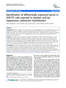
Figure Plots of 1the local FDR estimate for Golub data Plots of the local FDR estimate for Golub data x-axis: index of genes ordered along their p-values, y-axis: local FDR estimate. (a): raw values, (b): smooth estimates: moving average (discrete jumps), lowess (smooth curve), (c): zoom on the first 600 genes of (b): moving average (discrete jumps), lowess (upper smooth curve), q-value (lower thick smooth curve).

a high second order derivative, which corresponds to an abrupt change in the slope of the curve (see the examples of the following section). The second order derivative of the smoothed local FDR can be computed numerically using finite differences. As an interesting application of the local FDR, it is possible to compute the FDR associated with a class of genes or clones by summing up the local FDR estimate of each clone or gene: one may consider for example clones corresponding to the same gene, genes known involved in a given regulatory network, or gene from the same chromosomic region, and associate a FDR with the whole class. These genes do not need to have consecutive p-values. The following sections demonstrate how the local FDR can be useful using the data of well known experiments. Local FDR on Golub data set Golub [4] were interested in identifying genes that are differentially expressed in patients with two types of leukemias (ALL, AML). Gene expression levels were measured using Affymetrix high-density chips containing 6817 human genes. The learning set comprises 27 ALL cases and 11 AML cases.

Data are available in the R multtest package. We used the preprocessing proposed by the authors and the p-values based on random permutations of the ALL/AML labels on Welch t-statistics for each gene, Dudoit [5], on the 3051 remaining genes. m0 is estimated with bootstrap method as suggested by Storey and Tibshirani and implemented in the library GeneTS of software R.

n (i) for ordered genes and Figure 1(a) presents the FDR 1(b) presents the smooth curves obtained using lowess with a span of 0.2 and an adaptative moving average method. We can see that there is an abrupt change of the smoothed local FDR around gene number 500 which corresponds to a threshold t = 0.15 for the p-value. This may be an indication about the threshold. The Figure 1(c) presents a zoom of the Figure 1(b) for the first 600 p-values. We can see in Figure 1(c) that if we select the 438 (14%) top genes, we obtain a q-value equal to 0.0078 while the 438th gene has a local FDR equal to 0.027. It must be noticed that there is a big difference between the two measures of FDR because the numerous regulated genes with very small p-values have a great influence on the q-value, which is not the case of the local FDR (see Figure 1(c)). The p-values have been obtained using random permutations. Therefore the p-values are discrete with several genes possessing the same p-value. Therefore the values of

n (i, λ) may be equal to 0 because the difference FDR between two successive p-values is 0. The discrete structure of the p-values implies a departure from the theoretical continuous uniform distribution. This explains why the moving average smoothing creates discrete jumps which appear in Figure 1(c). If the distribution of the statistics under H0 is correct, the p-values are distributed as a uniform distribution over [0, 1]. The empirical distribution of the high observed p-val-




Table 1: p-value, q-value and local FDR estimates for three genes in Hedenfalk data.

p-value

rank

q-value

raw local FDR

smoothed local FDR

MSH2 PDCD5 CTGF

0.00005 0.00048 0.0036

8 47 159

0.013 0.022 0.049

0.013 0.013 0.176

0.010 0.033 0.098

0

500

1000

1500

2000

2500

3000

0.0

0

0.0

0.2

1

0.1

0.4

2

0.2

0.6

3

0.3

0.8

4

1.0

0.4

5

1.2

gene

0

500

1000

(a)

1500

(b)

2000

2500

3000

0

50

100

150

200

(c)

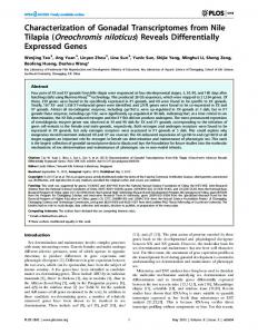
Figure Plots of 2the local FDR estimate for Hedenfalk data Plots of the local FDR estimate for Hedenfalk data x-axis: index of genes ordered along their p-values, y-axis: local FDR estimate. (a): raw values, (b): smooth estimates: moving average (discrete jumps), lowess (smooth curve), (c): zoom on the first 200 genes of (b): raw values (discrete jumps), moving average and lowess (smooth curves), q-value (lower thick smooth curve).

ues (say above 0.5) is far from the uniform distribution. There are several non-exclusive possibilities to explain this: more than 50% of the genes are differentially expressed, the gene results for non-differentially expressed are correlated or there is a technical problem in the random permutations of the Welch t-statistics. Local FDR on Breast Cancer data set Storey and Tibshirani [2], have analysed in detail data from Hedenfalk [6] on 15 microarrays on breast cancer. Using the same p-values, we have computed local FDR estimates. The three genes which have been analysed in detail by Storey and Tibshirani [2] are presented in Table 1.

One can see that the smooth local FDR estimate is generally greater than the q-value and gives a better idea of the probability that a gene is a false positive. For example, at the level of 5%, CTGF will be considered as differentially expressed on the basis of the q-value while it will be con-

sidered as non differentially expressed using the local FDR.

n (i) for ordered genes and Figure 2(a) presents the FDR 2(b) presents the smooth curves obtained using lowess with a span of 0.2 and moving average methods. The two smoothing methods give similar results. Setting λ = 0.5, Storey and Tibshirani [2] estimate that 67% of the 3170 genes in the data are not differentially expressed. The asymptote near 1 of the smooth curve supports this estimation. Local FDR on ApoAi data The goal of the study is to identify genes with altered expression in the livers of two lines of mice with very low HDL cholesterol levels compared to inbred control mice. The mouse model is the apolipoprotein AI (ApoAI) knock-out mice. ApoAI is a gene known to play a pivotal role in HDL metabolism. The statistical analysis is Page 4 of 9 (page number not for citation purposes)


0

1000

2000

3000

4000

5000

6000

0.4 0.0

0

0.0

0.2

1

0.2

0.4

2

0.6

3

0.8

0.6

1.0

4

1.2


0

1000

2000

(a)

3000

4000

5000

(b)

6000

0

10

20

30

40

50

(c)

Figure Plots of 3the local FDR estimate for Apo-AI data Plots of the local FDR estimate for Apo-AI data x-axis: index of clones ordered along their p-values, y-axis: local FDR estimate. (a): raw values, (b): smooth estimates: moving average (small discrete jumps), lowess (smooth curve), (c): zoom on the 50 first genes of (b): raw values (discrete jumps), moving average (smooth curve) lowess (upper rectangular curve), q-value (lower thick smooth curve).

described in Dudoit [7]. Height clones are expected to be differentially expressed between the control and the knock-out mices because they are clones of the ApoAI gene or of genes coregulated with ApoAI. The height clones are actually the 8 top clones detected by the statistical tests. However there are other following clones which seem statistically significant if we consider the q-value. We can see on the Figure 3(c) that the local FDR values are much higher than the q-values.

n (i) for ordered clones and Figure 3(a) presents the FDR Figure 3(b) presents the smooth curves obtained using lowess with a span of 0.2 and moving average methods. The two smoothing methods give different results at the two ends of the [0, 1] interval. The moving average method which uses a special adaptative algorithm for the ends gives a better smoothing. This is particularly important for the clones with a small p-value for which it is crucial to obtain good estimates of the probability of being false positives. The lowess smoothing does not work well for the 50 first clones. In this particular case the default smoothing parameter f = 0.2 is not well suited and should be lower. However if it is chosen too low, the smoothing will not fit well the rest of the curve. There are two clones of the gene Apo-AI. If we want to estimate the FDR of these two clones taken in a whole, we compute the mean of the smoothed local FDR of the two clones (the first and the height top clones) and obtain a local FDR for the gene Apo-AI, which is equal to

0 + 0.00048 = 0.00024 . This example shows that it is 2 possible to estimate the local FDR of any group of clones. This opportunity provided by the local FDR is certainly one of its major advantage with many potential applications.

Discussion The curve of the smoothed local FDR is an efficient tool to summarize the information about the number and the statistical significance of differentially expressed genes, and may also be used to give an indication about the validity of the statistical assumptions. Moreover it is a valuable tool to choose the threshold for separating the differentially expressed genes from the non-differentially expressed one: one can choose a value of t maximizing the second derivative. Alternatively one can use a cost function and choose the threshold that minimizes the mean cost for a given cost function: using cost of the experiment, cost of false positive gene validation and the profit of discovering a differentially expressed gene, it is direct to compute the optimal strategy for choosing the threshold. Note that a decision rule based on the local FDR would lead to a different set of selected genes than the usual one obtained by controlling the FDR. Consider the set of tests for which the local FDR is below 0.05, say. This set is not identical to the set identified by the standard criterion that FDR < 0.05. The local FDR is higher than the q-value. Therefore the first set is strictly included in the second




one. The local FDR rule is therefore more conservative than the usual FDR one.

extension from a test hypothesis procedure but can be very restrictive in a multiple testing procedure.

Conclusions

The status of the gene associated with the Pi is an unobserved value. It is the same framework as point process (see for example [8]). In fact we observe R(t) = V(t) + S(t) the sum of two counting processes. The first one V(t) is a counting process associated with non differentially expressed gene. Since the p-values under H0 are uniformly distributed, V(t) has a binomial distribution with parameter m0 and t. The intensity of V(t) is constant and proportional to m0. S(t) is the counting process associated with gene under H1 and very few can be said about its distribution. One may expect the intensity of S(t) to be decreasing with t. The false discovery rate is defined as:

The p-value gives the probability that a non differentially expressed gene would be as or more extreme than the gene under concern. The q-value indicates the estimated proportion of genes as or more extreme than the gene under concern that are a false positive. The local FDR gives the estimated proportion of genes around the gene under concern which are false positive. The latter may be used as the probability that the gene under concern is a false positive, taking into account the multiplicity of the test. One of the major interest of the local FDR is that it gives the opportunity to compute the FDR of any given group of clones (of the same gene) or genes pertaining to the same regulatory network or the same chromosome.

Methods Model Basically, the various procedures proposed in the literature aim to test the null hypothesis

H0(i) = {gene i is not differentially expressed}. Let consider a particular experiment. We observed the differential expression of the genes and compute the associated ordered p-values Pi. In the following we will use the classical property: the p-values corresponding to non differentially expressed genes are uniformly distributed over [0, 1]. Furthermore, we will assume, as often, that these pvalues are independent. However, the independence of the p-values of differentially expressed genes is not required. Consider a multiple testing situation in which m tests are being performed. Let m0 be the number of non differentially expressed genes. Let I(t) be the set of the genes having a p-value lower than t: I(t) = {i : Pi ≤ t} and R(t) = #I(t), its cardinal. Let V(t) = #[I(t) ∩ (i ∈ H0)] and S(t) = #[I(t) ∩ (i ∈ H1)]. Using a threshold t, the m genes can be classified according to the following 2 × 2 table 2: The Family Wise Error Rate (FWER) is defined to be FWER = P [V(t) ≥ 1]. A classical way to control FWER is given by the Bonferroni inequality. This quantity corresponds to the most direct

  V (t ) FDR(t ) = E  . max ( R ( t ), 1 )   It corresponds to the expected proportion of rejections that are incorrect. The BH procedure works as follows. Let P1 < …