Determining Bounds on Execution Times - Semantic Scholar

Determining Bounds on Execution Times Reinhard Wilhelm Informatik, Universität des Saarlandes Saarbrücken, Germany email: [email protected] Phone: +49 681 302 3434

2 Keywords: Real–Time Systems, WCET, Schedulability Analysis, Timing Analysis, Timing Anomalies, Static Program Analysis. Run-time guarantees play an important role in the area of embedded systems and especially hard real-time systems. These systems are typically subject to stringent timing constraints, which often result from the interaction with the surrounding physical environment. It is essential that the computations are completed within their associated time bounds; otherwise severe damages may result, or the system may be unusable. Therefore, a schedulability analysis has to be performed which guarantees that all timing constraints will be met. Schedulability analyses require upper bounds for the execution times of all tasks in the system to be known. These bounds must be safe, i.e., they may never underestimate the real execution time. Furthermore, they should be tight, i.e., the overestimation should be as small as possible. In modern microprocessor architectures, caches, pipelines, and all kinds of speculation are key features for improving (average-case) performance. Unfortunately, they make the analysis of the timing behaviour of instructions very difficult, since the execution time of an instruction depends on the execution history. A lack of precision in the predicted timing behaviour may lead to a waste of hardware resources, which would have to be invested in order to meet the requirements. For products which are manufactured in high quantities, e.g., in the automobile or telecommunications markets this would result in intolerable expenses. Subject of this chapter are one particular approach and the subtasks involved in computing safe and precise bounds on the execution times for real-time systems.

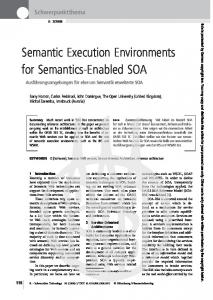
0.1 Introduction Hard real-time systems are subject to stringent timing constraints which are dictated by the surrounding physical environment. We assume that a real-time system consists of a number of tasks, which realize the required functionality. A schedulability analysis for this set of tasks and a given hardware has to be performed in order to guarantee that all the timing constraints of these tasks will be met (“timing validation”). Existing techniques for schedulability analysis require upper bounds for the execution times of all the system’s tasks to be known. These upper bounds are commonly called the worst-case execution times (WCETs), a misnomer that causes a lot of confusion and will therefore not be adopted in this presentation. In analogy, lower bounds on the execution time have been named best-case execution times, (BCET). These upper bounds (and lower bounds) have to be safe, i.e., they must never underestimate (overestimate) the real execution time. Furthermore, they should be tight, i.e., the overestimation (underestimation) should be as small as possible. Figure 0.1 depicts the most important concepts of our domain. The system shows a certain variation of execution times depending on the input data or different behaviour of the environment. In general, the state space is too large to exhaustively explore all possible executions and so determine the exact worst-case and best-case execution times. Some abstraction of the system is necessary to make a timing analysis of the system feasible. These abstractions loose information, and thus are responsible for the distance between WCETs and upper bounds and between BCETs and lower bounds.

0.1. INTRODUCTION

3

predictability w.c. guarantee w.c. performance

0

lower bound

best case

worst case

upper bound

t

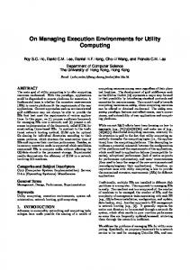
variation of execution time Figure 1: Basic notions concerning timing analysis of systems. How much is lost depends both on the methods used for timing analysis and on system properties, such as the hardware architecture and the cleanness of the software. So, the two distances mentioned above, termed upper predictability and lower predictability can be seen as a measure for the timing predictability of the system. Experience has shown that the two predictabilities can be quite different, cf. [HLTW03]. The methods used to determine upper bounds and lower bounds are the same. We will concentrate on the determination of upper bounds unless otherwise stated. Methods to compute sharp bounds [PK89, PS91] for processors with fixed execution times for each instruction have long been established. However, in modern microprocessor architectures caches, pipelines, and all kinds of speculation are key features for improving (average-case) performance. Caches are used to bridge the gap between processor speed and the access time of main memory. Pipelines enable acceleration by overlapping the executions of different instructions. The consequence is that the execution time of individual instructions, and thus the contribution of one execution of an instruction to the program’s execution time can vary widely. The interval of execution times for one instruction is bounded by the execution times of the following two cases: • The instruction goes “smoothly” through the pipeline; all loads hit the cache, no pipeline hazard happens, i.e., all operands are ready, no resource conflicts with other currently executing instructions exist. • “Everything goes wrong”, i.e., instruction and/or operand fetches miss the cache, resources needed by the instruction are occupied, etc. Figure 2 shows the different paths through a multiply instruction of a PowerPC processor. The instruction-fetch phase may find the instruction in the cache (cache hit), in which case it takes 1 cycle to load it. In the case of a cache miss, it may take something like 30 cycles to load the memory block containing the instruction into the cache. The instruction needs an arithmetic unit, which may be occupied by a preceding instruction. Waiting for the unit to become free may take up to 19 cycles. This latency would not occur, if the instruction fetch had missed the cache, because the cache-miss penalty of

4

Fetch

Issue

Execute

Retire

I−Cache miss?

Unit occupied?

Multicycle?

Pending instructions? 6

19

4

1 6

3

No

30

6

Yes 1 3

6 41

Figure 2: Different paths through the execution of a multiply instruction. Unlabeled transitions take 1 cycle. 30 cycles has allowed any preceding instruction to terminate its arithmetic operation. The time it takes to multiply two operands depends on the size of the operands; for small operands, one cycle is enough, for larger, three are needed. When the operation has finished, it has to be retired in the order it appeared in the instruction stream. The processor keeps a queue for instructions waiting to be retired. Waiting for a place in this queue may take up to 6 cycles. On the dashed path, where the execution always takes the fast way, its overall execution time is 4 cycles. However, on the dotted path, where it always takes the slowest way, the overall execution time is 41 cycles. We will call any increase in execution time during an instruction’s execution a timing accident and the number of cycles by which it increases the timing penalty of this accident. Timing penalties for an instruction can add up to several hundred processor cycles. Whether the execution of an instruction encounters a timing accident depends on the execution state, e.g., the contents of the cache(s), the occupancy of other resources, and thus on the execution history. It is therefore obvious that the attempt to predict or exclude timing accidents needs information about the execution history. For certain classes of architectures, namely those without timing anomalies, excluding timing accidents means decreasing the upper bounds. However, for those with timing anomalies this assumption is not true.

0.1.1 Tool Architecture and Algorithm A more or less standard architecture for timing-analysis tools has emerged [HWH95, TFW00, Erm03]. Fig. 3 shows one instance of this architecture. A first phase, de-

0.1. INTRODUCTION

Figure 3: The architecture of the aiT timing-analysis tool.

5

6 picted on the left, predicts the behaviour of processor components for the instructions of the program. It usually consists of a sequence of static program analyses of the program. They altogether allow to derive safe upper bounds for the execution times of basic blocks. A second phase, the column on the right, computes an upper bound on the execution times over all possible paths of the program. This is realized by mapping the control flow of the program to an Integer Linear Program and solving this by appropriate methods. This architecture has been successfully used to determine precise upper bounds on the execution times of real-time programs running on processors used in embedded systems [AFMW96, FMW99, FHL+ 01, TSH+ 03, HLTW03]. A commercially available tool, aiT by AbsInt, cf. http://www.absint.de/wcet.htm, was implemented and is used in the aeronautics and automotive industries. The structure of the first phase, processor-behavior prediction, often called microarchitecture analysis, may vary depending on the complexity of the processor architecture. A first, modular approach would be the following: 1. Cache-behavior prediction determines statically and approximately the contents of caches at each program point. For each access to a memory block, it is checked, whether the analysis can safely predict a cache hit. Information about cache contents can be forgotten after the cache analysis. Only the miss/hit information is needed by the pipeline analysis, 2. Pipeline-behavior prediction analyzes, how instructions pass through the pipeline taking cache-hit or miss information into account. The cache-miss penalty is assumed for all cases, where a cache hit can not be guaranteed. At the end of simulating one instruction, the pipeline analysis continues with only those states that show the locally maximal execution times. All others can be forgotten.

0.1.2 Timing Anomalies Unfortunately, this approach is not safe for many processor architectures. Most powerful microprocessors have so-called timing anomalies. Timing anomalies are contraintuitive influences of the (local) execution time of one instruction on the (global) execution time of the whole program. The interaction of several processor features can interact in such a way that a locally faster execution of an instruction can lead to a globally longer execution time of the whole program. For example, a cache miss contributes the cache-miss penalty to the execution time of a program. It was, however, observed for the MCF 5307 [RSW02], that a cache miss may actually speed up program execution. Since the MCF 5307 has a unified cache and the fetch and execute pipelines are independent, the following can happen: A data access that is a cache hit is served directly from the cache. At the same time, the fetch pipeline fetches another instruction block from main memory, performing branch prediction and replacing two lines of data in the cache. These may be reused later on and cause two misses. If the data access was a cache miss, the instruction fetch pipeline may not have fetched those two lines, because the execution pipeline may have resolved a misprediction before those lines were fetched.

0.1. INTRODUCTION

7

The general case of a timing anomaly is the following. Different assumption about the processor’s execution state, e.g. the fact that the instruction is or is not in the instruction cache, will result in a difference ∆Tlocal of the execution time of the instruction between these two cases. Either assumption may lead to a difference ∆T of the global execution time compared to the other one. We say that a timing anomaly occurs if either ∆Tlocal < 0 i.e., the instruction executes faster, and ∆T < ∆Tlocal , the overall execution is accelerated by more than the acceleration of the instruction, or ∆T > 0 , the program runs longer than before. ∆Tlocal > 0 i.e., the instruction takes longer to execute, and ∆T > ∆Tlocal i.e., the overall execution is extended by more than the delay of the instruction, or ∆T < 0 i.e., the overall execution of the program takes less time to execute than before. The case ∆Tlocal < 0 ∧ ∆T > 0 is a critical case for our timing analysis. It makes it impossible to use local worst cases for the calculation of the program’s execution time. The analysis has to follow all possible paths as will be explained in Section 0.3.

0.1.3 Contexts The contribution of an individual instruction to the total execution time of a program may vary widely depending on the execution history. For example, the first interation of a loop typically loads the caches, and later iterations profit from the loaded memory blocks being in the caches. In this case, the execution of an instruction in a first iteration encounters one or more cache misses and pays with the cache-miss penalty. Later executions, however, will execute much faster because they hit the cache. A similar observation holds for dynamic branch predictors. They may need a few iterations until they stabilize and predict correctly. Therefore, precision is increased if instructions are considered in their control–flow context, i.e., the way control reached them. Contexts are associated with basic blocks, i.e., maximally long straight-line code sequences that can be only entered at the first instruction and left at the last. They indicate through which sequence of function calls and loop iterations control arrived at the basic block. Thus, when analyzing the cache behavior of a loop, precision can be increased by regarding the first iteration of the loop and all other iterations separately; more precisely, to unroll the loop once and then analyze the resulting code. 1 Definition 1 Let p be a program with set of functions P = {p1 , p2 , . . . , pn } and set of loops L = {l1 , l2 , . . . , ln }. A word c over the alphabet P ∪ L × IN is called a context for 1 Actually, this unrolling transformation need not be really performed, but can be incorporated into the iteration strategy of the analyzer. So, we talk of virtual unrolling the loops.

8 a basic block b, if b can be reached by calling the functions and iterating through the loops in the order given in c. Even, if all loops have static loop bounds and recursion is also bounded, there are in general too many contexts to consider them exhaustively. A heuristics is used to keep relevant contexts apart and summarize the rest conservatively, if their influence on the behaviour of instructions does not significantly differ. Experience has shown [TSH+ 03], that a few first iterations and recursive calls are sufficient to “stabilize” the behavior information, as the above example indicates, and that the right differentiation of contexts is decisive for the precision of the prediction [MAWF98]. A particular choice of contexts transforms the call and the control flow graph into a context-extended control-flow graph by virtually unrolling the loops and virtually inlining the functions as indicated by the contexts. The formal treatment of this concept is quite involved and shall not be given here. It can be found in [The02].

0.2 Cache-Behaviour Prediction Abstract Interpretation [CC77] is used to compute invariants about cache contents. How the behavior of programs on processor pipelines is predicted follows in Section 0.3.

0.2.1 Cache Memories A cache can be characterized by three major parameters: • capacity is the number of bytes it may contain. • line size (also called block size) is the number of contiguous bytes that are transferred from memory on a cache miss. The cache can hold at most n = capacity/line size blocks. • associativity is the number of cache locations where a particular block may reside. n/associativity is the number of sets of a cache. If a block can reside in any cache location, then the cache is called fully associative. If a block can reside in exactly one location, then it is called direct mapped. If a block can reside in exactly A locations, then the cache is called A-way set associative. The fully associative and the direct mapped caches are special cases of the A-way set associative cache where A = n and A = 1, resp. In the case of an associative cache, a cache line has to be selected for replacement when the cache is full and the processor requests further data. This is done according to a replacement strategy. Common strategies are LRU (Least Recently Used), FIFO (First In First Out), and random. The set where a memory block may reside in the cache is uniquely determined by the address of the memory block, i.e., the behavior of the sets is independent of each other. The behavior of an A-way set associative cache is completely described by the

0.2. CACHE-BEHAVIOUR PREDICTION

9

behavior of its n/A fully associative sets. This holds also for direct mapped caches where A = 1. For the sake of space, we restrict our description to the semantics of fully associative caches with LRU replacement strategy. More complete descriptions that explicitly describe direct mapped and A-way set associative caches can be found in [Fer97, FMW99].

0.2.2 Cache Semantics In the following, we consider a (fully associative) cache as a set of cache lines L = {l1 , . . . , ln } and the store as a set of memory blocks S = {s1 , . . . , sm }. To indicate the absence of any memory block in a cache line, we introduce a new element I; S′ = S ∪ {I}. Definition 2 (concrete cache state) A (concrete) cache state is a function c : L → S′ . Cc denotes the set of all concrete cache states. The initial cache state cI maps all cache lines to I. If c(li ) = sy for a concrete cache state c, then i is the relative age of the memory block according to the LRU replacement strategy and not necessarily the physical position in the cache hardware. The update function describes the effect on the cache of referencing a block in memory. The referenced memory block sx moves into l1 if it was in the cache already. All memory blocks in the cache that had been used more recently than sx increase their relative age by one, i.e., they are shifted by one position to the next cache line. If the referenced memory block was not yet in the cache, it is loaded into l1 after all memory blocks in the cache have been shifted and the ‘oldest’, i.e., least recently used memory block, has been removed from the cache if the cache was full. Definition 3 (cache update) A cache update function U : Cc × S → Cc determines the new cache state for a given cache state and a referenced memory block. Updates of fully associative caches with LRU replacement strategy are pictured as in Figure 4. Control Flow Representation We represent programs by control flow graphs consisting of nodes and typed edges. The nodes represent basic blocks. A basic block is a sequence (of fragments) of instructions in which control flow enters at the beginning and leaves at the end without halt or possibility of branching except at the end. For cache analysis, it is most convenient to have one memory reference per control flow node. Therefore, our nodes may represent the different fragments of machine instructions that access memory. For non-precisely determined addresses of data references, one can use a set of possibly referenced memory blocks. We assume that for each basic block, the sequence of references to memory is known (This is appropriate for instruction caches and can be too restricted for data caches and combined caches. See

10

z y x t

s z y x

z s x t

s z x t

"young"

Age "old"

[s ] Figure 4: Update of a concrete fully associative (sub-) cache. [Fer97, AFMW96] for weaker restrictions.), i.e., there exists a mapping from control flow nodes to sequences of memory blocks: L : V → S∗ . We can describe the effect of such a sequence on a cache with the help of the update function U. Therefore, we extend U to sequences of memory references by sequential composition: U(c, hsx1 , . . . , sxy i) = U(. . . (U(c, sx1 )) . . . , sxy ). The cache state for a path (k1 , . . . , k p ) in the control flow graph is given by applying U to the initial cache state cI and the concatenation of all sequences of memory references along the path: U(cI , L(k1 ). ... .L(k p )). The Collecting Semantics of a program gathers at each program point the set of all execution states, which the program may encounter at this point during some execution. A semantics on which to base a cache analysis has to model cache contents as part of the execution state. One could thus compute the collecting semantics and project the execution states onto their cache components to obtain the set of all possible cache contents for a given program point. However, the collecting semantics is in general not computable. Instead, one restricts the standard semantics to only those program constructs, which involve the cache, i.e., memory references. Only they have an effect on the cache modelled by the cache update function, U. This coarser semantics may execute program paths which are not executable in the start semantics. Therefore, the Collecting Cache Semantics of a program computes a superset of the set of all concrete cache states occurring at each program point. Definition 4 (Collecting Cache Semantics) The Collecting Cache Semantics of a program is Ccoll (p) = {U(cI , L(k1 ). ... .L(kn )) | (k1 , . . . , kn ) path in the CFG leading to p} This collecting semantics would be computable, although often of enormous size. Therefore, another step abstracts it into a compact representation, so called abstract


11

cache states. Note that every information drawn from the abstract cache states allows to safely deduce information about sets of concrete cache states, i.e., only precision may be reduced in this two step process. Correctness is guaranteed. Abstract Semantics The specification of a program analysis consists of the specification of an abstract domain and of the abstract semantic functions, mostly called transfer functions. The least upper bound operator of the domain combines information when control flow merges. We present two analyses. The must analysis determines a set of memory blocks that are in the cache at a given program point whenever execution reaches this point. The may analysis determines all memory blocks that may be in the cache at a given program point. The latter analysis is used to determine the absence of a memory block in the cache. The analyses are used to compute a categorization for each memory reference describing its cache behavior. The categories are described in Table 1. Category Abb. Meaning always hit ah The memory reference will always result in a cache hit. always miss am The memory reference will always result in a cache miss. not classified nc The memory reference could neither be classified as ah nor am. Table 1: Categorizations of memory references and memory blocks. The domains for our abstract interpretations consist of abstract cache states: Definition 5 (abstract cache state) An abstract cache state cˆ : L → 2S maps cache lines to sets of memory blocks. Cˆ denotes the set of all abstract cache states. The position of a line in an abstract cache will, as in the case of concrete caches, denote the relative age of the corresponding memory blocks. Note, however, that the domains of abstract cache states will have different partial orders and that the interpretation of abstract cache states will be different in the different analyses. The following functions relate concrete and abstract domains. An extraction function, extr, maps a concrete cache state to an abstract cache state. The abstraction function, abstr, maps sets of concrete cache states to their best representation in the domain of abstract cache states. It is induced by the extraction function. The concretization function, concr, maps an abstract cache state to the set of all concrete cache states represented by it. It allows to interpret abstract cache states. It is often induced by the abstraction function, cf. [NNH99]. Definition 6 (extraction, abstraction, concretization functions) The extraction function extr : Cc → Cˆ forms singleton sets from the images of the concrete cache states it is applied to, i.e., extr(c)(li ) = {sx } if c(li ) = sx . F The abstraction function abstr : 2Cc → Cˆ is defined by abstr(C) = {extr(c) | c ∈ C} The concretization function concr : Cˆ → 2Cc is defined by concr(c) ˆ = {c | extr(c) ⊑ c}. ˆ

12 So much of commonalities of all the domains to be designed. Note, that all the constructions are parameterized in ⊔ and ⊑. The transfer functions, the abstract cache update functions, all denoted Uˆ , will describe the effects of a control flow node on an element of the abstract domain. They will be composed of two parts, 1. “refreshing” the accessed memory block, i.e., inserting it into the youngest cache line, 2. “aging” some other memory blocks already in the abstract cache. Termination of the analyses There are only a finite number of cache lines and for each program a finite number of memory blocks. This means, that the domain of abstract cache states cˆ : L → 2S is finite. Hence, every ascending chain is finite. Additionally, the abstract cache update functions, Uˆ , are monotonic. This guarantees that all the analyses will terminate. Must Analysis As explained above, the must analysis determines a set of memory blocks that are in the cache at a given program point whenever execution reaches this point. Good information, in the sense of valuable for the prediction of cache hits, is the knowledge that a memory block is in this set. The bigger the set, the better. As we will see, additional information will even tell how long it will at least stay in the cache. This is connected to the “age” of a memory block. Therefore, the partial order on the must– domain is as follows. Take an abstract cache state c. ˆ Above cˆ in the domain, i.e., less precise, are states where memory blocks from cˆ are either missing or are older than in c. ˆ Therefore, the ⊔-operator applied to two abstract cache states cˆ1 and cˆ2 will produce a state cˆ containing only those memory blocks contained in both, and will give them the maximum of their ages in cˆ1 and cˆ2 (see Figure 6). The positions of the memory blocks in the abstract cache state are thus the upper bounds of the ages of the memory blocks in the concrete caches occurring in the collecting cache semantics. Concretization of an abstract cache state, c, ˆ produces the set of all concrete cache states, which contain all the memory blocks contained in cˆ with ages not older than in c. ˆ Cache lines not filled by these are filled with other memory blocks. We use the abstract cache update function depicted in Figure 5. Let us argue the correctness of this update function. The following theorem formulates the soundness of the must-cache analysis. Theorem 1 Let n be a program point, cîn the abstract cache state at the entry to n, s a memory line in cîn with age k. (i) For each 1 ≤ k ≤ A there are at most k memory lines in lines 1, 2, . . . , k (ii) On all paths to n, s is in cache with age at most k. The solution of the must analysis problem is interpreted as follows: Let cˆ be an abstract cache state at some program point. If sx ∈ c(l ˆ i ) for a cache line li then sx will definitely be in the cache whenever execution reaches this program point. A reference to sx is categorized as always hit (ah). There is even a stronger interpretation of the fact


13

{ x} {} {s, t } { y}

{s } {x } {t } {y}

"young"

Age "old"

[s ] Figure 5: Update of an abstract fully associative (sub-) cache.

{c} {e } {a} {d }

{ a} {} {c, f } {d}

"intersection + maximal age" {} {} {a,c } {d }

Figure 6: Combination for must analysis

14 {c} {e } {a} {d }

{ a} { c, f } {} {d}

"union + minimal age" {a,c} {e, f } {} {d }

Figure 7: Combination for may analysis that sx ∈ c(l ˆ i ). sx will stay in the cache at least for the next n − i references to memory blocks that are not in the cache or are older than the memory blocks in c, ˆ whereby sa is older than sb means: ∃li , l j : sa ∈ c(l ˆ i ), sb ∈ c(l ˆ j ), i > j. May Analysis To determine, if a memory block sx will never be in the cache, we compute the complimentary information, i.e., sets of memory blocks that may be in the cache. “Good” information is that a memory block is not in this set, because this memory block can be classified as definitely not in the cache whenever execution reaches the given program point. Thus, the smaller the sets are, the better. Additionally, the older blocks will reach the desired situation to be removed from the cache faster than the younger ones. Therefore, the partial order on this domain is as follows. Take some abstract cache state c. ˆ Above cˆ in the domain, i.e., less precise, are those states which contain additional memory blocks or where memory blocks from cˆ are younger than in c. ˆ Therefore, the ⊔-operator applied to two abstract cache states cˆ1 and cˆ2 will produce a state cˆ containing those memory blocks contained in cˆ1 or cˆ2 and will give them the minimum of their ages in cˆ1 and cˆ2 (see Figure 7). The positions of the memory blocks in the abstract cache state are thus the lower bounds of the ages of the memory blocks in the concrete caches occurring in the collecting cache semantics. The solution of the may analysis problem is interpreted as follows: The fact that sx is in the abstract cache cˆ means that sx may be in the cache during some execution when the program point is reached. If sx is not in c(l ˆ i ) for any li then it will definitely be not in the cache on any execution. A reference to sx is categorized as always miss (am).

0.3 Pipeline Analysis Pipeline analysis attempts to find out how instructions move through the pipeline. In particular, it determines how many cycles they spend in the pipeline. This largely depends on the timing accidents the instructions suffer. Timing accidents during pipelined

0.3. PIPELINE ANALYSIS

15

executions can be of several kinds. Cache misses during instruction or data load stall the pipeline for as many cycles as the cache miss penalty indicates. Functional units that an instruction needs may be occupied. Queues into which the instruction may have to be moved may be full, and prefetch queues, from which instructions have to be loaded, may be empty. The bus needed for a pipeline phase may be occupied by a different phase of another instruction. Again, for a architectures without timing anomalies we can use a simplified picture, in which the task is to find out which timing accidents can be safely excluded, because each excluded accident allows to decrease the bound for the execution time. Accidents that can not be safely excluded are assumed to happen. A cache analysis as described in Section 0.2 has annotated the instructions with cache-hit information. This information is used to exclude pipeline stalls at instruction or data fetches. We will explain pipeline analysis in a number of steps starting with concretepipeline execution. A pipeline goes through a number of pipeline phases and consumes a number of cycles when it executes a sequence of instructions; in general, a different number of cycles for different initial execution states. The execution of the instructions in the sequence overlaps in the instruction pipeline as far as the data dependences between instructions permit it and if the pipeline conditions are statisfied. Each execution of a sequence of instructions starting in some initial state produces one trace, i.e., sequence of execution states. The length of the trace is the number of cycles this execution takes. Thus, concrete execution can be viewed as applying a function function exec (b : basic block, s : pipeline state) t : trace that executes the instruction sequence of basic block b starting in concrete pipeline state s producing a trace t of concrete states. last(t) is the final state when executing b. It is the initial state for the successor block to be executed next. So far, we talked about concrete execution on a concrete pipeline. Pipeline analysis regards abstract execution of sequences of instructions on abstract (models of) pipelines. The execution of programs on abstract pipelines produces abstract traces, i.e., sequences of abstract states, where some information contained in the concrete states may be missing. There are several types of missing information. • The cache analysis in general has incomplete information about cache contents. • The latency of an arithmetic operation, if it depends on the operand sizes, may be unknown. It influences the occupancy of pipeline units. • The state of a dynamic branch predictor changes over iterations of a loop and may be unknown for a particular iteration. • Data dependences can not safely be excluded because effective addresses of operands are not always statically known. Simple Architectures without Timing Anomalies In a first step, we assume a simple processor architecture, with in-order execution and without timing anomalies, i.e., architectures, where local worst cases contribute to the

16 program’s global execution time, cf. 0.1.2. Also, it is safe to assume the local worst cases for unknown information. For both of them the corresponding timing penalties are added. For example, the cache miss penalty has to be added for instruction fetch of an instruction in the two cases, that a cache miss is predicted or that neither a cache miss nor a cache hit can be predicted. The result of the abstract execution of an instruction sequence for a given initial abstract state is again one trace; however, possibly of a greater length and thus an upper bound properly bounding the execution time from above. Because worst cases were assumed for all uncertainties, this number of cycles is a safe upper bound for all executions of the basic block starting in concrete states represented by this initial abstract state. The Algorithm for pipeline analysis is quite simple. It uses a function function exec ˆ (b : cache-annotated basic block, sˆ : abstract pipeline state) tˆ : abstract trace that executes the instruction sequence of basic block b, annotated with cache information, starting in the abstract pipeline state sˆ and producing a trace tˆ of abstract states. This function is applied to each basic block b in each of its contexts and the empty pipeline state sˆ0 corresponding to a flushed pipeline. Therefore, a linear traversal of the cache-annotated context-extended Basic-Block Graph suffices. The result is a trace for the instruction sequence of the block, whose length is an upper bound for the execution time of the block in this context. Note, that it still makes sense to analyze a basic block in several contexts because the cache information for them may be quite different. Note, that this algorithm is simple and efficient, but not necessarily very precise. Starting with a flushed pipeline at the beginning of the basic block is safe, but it ignores the potential overlap between consecutive basic blocks. A more precise algorithm is possible. The problem is with basic blocks having several predecessor blocks. Which of their final states should be selected as initial state of the successor block? First solution involves working with sets of states for each pair of basic block and context. Then, one analysis of each basic block and context would be performed for each of the initial states. The resulting set of final states would be passed on to successor blocks, and the maximum of the trace lengths would be taken as upper bound for this basic block in this context. Second solution would work with a single state per basic block and context and would combine the set of predecessor final states conservatively to the initial state for the successor. Processors with Timing Anomalies In the next step, we assume more complex processors, including those with out-oforder execution. They typically have timing anomalies. Our assumption above, i.e., that local worst cases contribute worst-case times to the global execution times, is no more valid. This forces us to consider several paths, wherever uncertainty in the abstract execution state does not allow to take a decision between several successor states. Note, that the absence of information leads from the deterministic concrete


17

Fetch

Issue

Execute

Retire

I−Cache miss?

Unit occupied?

Multicycle?

Pending instructions? 6

19

4

1 6

3

No

6

30

6

Yes 1 3

6 41

Figure 8: Different paths through the execution of a multiply instruction. Decisions inside the boxes can not be deterministically taken based on the abstract execution state because of missing information.

pipeline to an abstract pipeline that is non-deterministic. This situation is depicted in Fig. 8. It demonstrates two cases of missing information in the abstract state. First, the abstract state lacks the information whether the instruction is in the I-cache. Pipeline analysis has to follow both cases in case of instruction fetch, because it could turn out that the I-cache miss, in fact, is not the global worst case. Secondly, the abstract state does not contain information about the size of the operands. We also have to follow both paths. The dashed paths have to be explored to obtain the execution times for this instruction. Depending on the architecture, we may be able to conservatively assume the case of large operands and surpress some paths. The algorithm has to combine cache and pipeline analysis because of the interference between both, which actually is the reason for the existence of the timing anomalies. For the cache analysis, it uses the abstract cache states discussed in Section 0.2. For the pipeline part, it uses analysis states, which are sets of abstract pipeline states, i.e. sets of states of the abstract pipeline. The question arises whether an abstract cache state is to be combined with an analysis state ss ˆ or an individual one with each of the abstract pipeline states in ss. ˆ So, there could be one abstract cache state for ss ˆ representing the concrete cache contents for all abstract pipeline states in ss, ˆ or there could be one abstract cache state per abstract pipeline state in ss. ˆ The first choice saves memory during the analysis, but loses precision. This is because different pipeline states may cause different memory accesses and thus cache contents, which have to be merged into the one abstract state thereby losing information. The second choice is more precise but requires more memory during the analysis. We choose the second

18

Figure 9: Possible pipeline states in a basic block alternative and thus define a new domain of analysis states Aˆ of the following type: ˆ ˆ Aˆ = 2S×C

(1)

Sˆ = set of abstract pipeline states Cˆ = set of abstract cache states

(2) (3)

The Algorithm again uses a new function exec ˆ c. function exec ˆ c (b : basic block, aˆ : analysis state) Tˆ : set of abstract trace, which analyzes a basic block b starting in an analysis state aˆ consisting of pairs of abstract pipeline states and abstract cache states. As a result it will produce a set of abstract traces. The algorithm is as follows: Algorithm Pipeline-Analysis Perform fixpoint iteration over the context-extended Basic-Block Graph: For each basic block b in each of its contexts c, and for the initial analysis state a, ˆ compute exec ˆ c (b, a) ˆ yielding a set of traces {tˆ1 , tˆ2 , . . . , tˆm }. max({|tˆ1 |, |tˆ2 |, . . . , |tˆm |} is the bound for this basic block in this context. The set of output states {last(tˆ1 ), last(tˆ2 ), . . . , last(tˆm )} will be passed on to the successor block(s) in context c as initial states. Basic blocks (in some context) having more than one predecessor receive the union of the set of output states as initial states. The abstraction we use as analysis states is a set of abstract pipeline states, since the number of possible pipeline states for one instruction is not too big. Hence, our abstraction computes an upper bound to the collecting semantics. The abstract update for an analysis state aˆ is thus the application of the concrete update on each abstract pipeline state in aˆ extended with the possibility of multiple successor states in case of uncertainties. Figure 9 shows the possible pipeline states for a basic block in this example. Such pictures are shown by aiT tool upon special demand. The large dark grey boxes correspond to the instructions of the basic block, and the smaller rectangles in them stand for individual pipeline states. Their cyclewise evolution is indicated by the strokes


19

connecting them. Each layer in the trees corresponds to one CPU cycle. Branches in the trees are caused by conditions that could not be statically evaluated, e.g. a memory access with unknown address in presence of memory areas with different access times. On the other hand, two pipeline states fall together when details they differ in leave the pipeline. This happened, for instance, at the end of the second instruction, reducing the number of states from four to three. The update function belonging to an edge (v, v′ ) of the control-flow graph updates each abstract pipeline state separately. When the bus unit is updated, the pipeline state may split into several successor states with different cache states. The initial analysis state is a set of empty pipeline states plus a cache that represents a cache with unknown content. There can be multiple concrete pipeline states in the initial states, since the adjustment of internal to external clock of the processor is not known in the beginning and every possibility (aligned, one cycle apart, etc) has to be considered. Thus prefetching must start from scratch, but pending bus requests are ignored. To obtain correct results, they must be taken into account by adding a fixed penalty to the calculated upper bounds.

0.3.1 Pipeline Modeling The basis for pipeline analysis is a model of an abstract version of the processor pipeline, which is conservative with respect to the timing behavior, i.e., times predicted by the abstract pipeline must never be lower than those observed in concrete executions. Some terminology is needed to avoid confusion. Processors have concrete pipelines, which may be described in some formal language, e.g. VHDL. If this is the case, there exists a formal model of the pipeline. Our abstraction step, by which we eliminate many components of a concrete pipeline that are not relevant for the timing behavior lead us to an abstract pipeline. This may again be described in a formal language, e.g. VHDL, and thus have a formal model. Deriving an abstract pipeline is a complex task. It is demonstrated for the Motorola ColdFire processor, a processor quite popular in the aeronautics and the submarine industry. The presentation follows closely that of [LTH02]2 . The ColdFire MCF 5307 Pipeline The pipeline of the ColdFire MCF 5307 consists of a fetch pipeline that fetches instructions from memory (or the cache), and an execution pipeline that executes instructions, cf. Figure 10. Fetch and execution pipelines are connected and as far as speed is concerned decoupled by a FIFO instruction buffer that can hold at most 8 instructions. The MCF 5307 accesses memory through a bus hierarchy. The fast pipelined K-bus connects the cache and an internal 4KB SRAM area to the pipeline. Accesses to this bus are performed by the IC1/IC2 and the AGEX and DSOC stages of the pipeline. On the next level, the M-Bus connects the K-Bus to the internal peripherals. This bus runs at the external bus frequency, while the K-Bus is clocked with the faster internal core 2 The model of the abstract pipeline of the MCF 5307 has been derived by hand. A computer-supported derivation would have been preferable. Ways to develop this are subject of actual research.

20 clock. The M-Bus connects to the external bus, which accesses off-chip peripherals and memory. The fetch pipeline performs branch prediction in the IED stage, redirecting fetching long before the branch reaches the execution stages. The fetch pipeline is stalled if the instruction buffer is full, or if the execution pipeline needs the bus for a memory access. All these stalls cause the pipeline to wait for one cycle. After that, the stall condition is checked again. The fetch pipeline is also stalled if the memory block to be fetched is not in the cache (cache miss). The pipeline must wait until the memory block is loaded into the cache and forwarded to the pipeline. The instructions that are already in the later stages of the fetch pipeline are forwarded to the instruction buffer. The execution pipeline finishes the decoding of instructions, evaluates their operands, and executes the instructions. Each kind of operation follows a fixed schedule. This schedule determines, how many cycles the operation needs and in which cycles memory is accessed3 . The execution time varies between 2 cycles and several dozen cycles. Pipelining admits a maximum overlap of 1 cycle between consecutive instructions: the last cycle of each instruction may overlap with the first of the next one. In this first cycle, no memory access and no control-flow alteration happen. Thus, cache and pipeline cannot be affected by two different instructions in the same cycle. The execution of an instruction is delayed if memory accesses lead to cache misses. Misaligned accesses lead to small time penalties of 1–3 cycles. Store operations are delayed if the distance to the previous store operation is less than 2 cycles. (This does not hold if the previous store operation was issued by a MOVEM instruction.) The start of the next instruction is delayed if the instruction buffer is empty.

0.3.2 Formal Models of Abstract Pipelines An abstract pipeline can be seen as a big finite state machine, which makes a transition on every clock cycle. The states of the abstract pipeline, although greatly simplified still contain all timing relevant information of the processor. The number of transitions it takes from the beginning of the execution of an instruction until its end gives the execution time of that instruction. The abstract pipeline although greatly reduced by leaving out irrelevant components still is a really big finite state machine, but it has structure. Its states can be naturally decomposed into components according to the architecture. This makes it easier to specify, verify, and implement a model of an abstract pipeline. In the formal approach presented here, an abstract pipeline state consists of several units with inner states that communicate with one another and the memory via signals, and evolve cycle-wise according to their inner state and the signals received. Thus, the means of decomposition are units and signals. Signals may be instantaneous, meaning that they are received in the same cycle as they are sent, or delayed, meaning that they are received one cycle after they have been sent. Signals may carry data, e.g. a fetch address. Note that these signals are only 3 In fact, there are some instructions like MOVEM whose execution schedule depends on the value of an argument as immediate constant. These instructions can be taken into account by special means.


Instruction Fetch Pipeline (IFP)

Operand Execution Pipeline (OEP)

IAG

Instruction Address Generation

IC1

Instruction Fetch Cycle 1

IC2

Instruction Fetch Cycle 2

IED

Instruction Early Decode

IB

FIFO Instruction Buffer

DSOC

Decode & Select, Operand Fetch

AGEX

Address Generation, Execute

21

Address [31:0]

Figure 10: The pipeline of the Motorola ColdFire 5307 processor

Data[31:0]

22 part of the formal pipeline model. They may or may not correspond to real hardware signals. The instantaneous signals between units are used to transport information between the units. The state transitions are coded in the evolution rules local to each unit. Figure 11 shows the formal pipeline model for the ColdFire MCF 5307. It consists of the following units: IAG (instruction address generation), IC1 (instruction fetch cycle 1), IC2 (instruction fetch cycle 2), IED (instruction early decode), IB (instruction buffer), EX (execution unit), SST (store stall timer). In addition, there is a bus unit modeling the busses that connect the CPU, the static RAM, the cache, and the main memory. The signals between these units are shown as arrows. Most units directly correspond to a stage in the real pipeline. However, the SST unit is used to model the fact that two stores must be separated by at least two clock cycles. It is implemented as a (virtual) counter. The two stages of the execution pipeline are modeled by a single stage, EX, because instructions can only overlap by one cycle. The inner states and emitted signals of the units evolve in each cycle. The complexity of this state update varies from unit to unit. It can be as simple as a small table, mapping pending signals and inner state to a new state and signals to be emitted, e.g. for the IAG unit and the IC1 unit. It can be much more complicated, if multiple dependencies have to be considered, e.g. the instruction reconstruction and branch prediction in the IED stage. In this case, the evolution is formulated in pseudo code. Full details on the model can be found in [The04].

0.3.3 Pipeline States Abstract Pipeline States are formed by combining the inner states of IAG, IC1, IC2, IED, IB, EX, SST, and bus unit plus additional entries for pending signals into one overall state. This overall state evolves from one cycle to the next. Practically, the evolution of the overall pipeline state can be implemented by updating the functional units one by one in an order that respects the dependencies introduced by input signals and the generation of these signals.

Update Function for Pipeline States. For pipeline modeling, one needs a function that describes the evolution of the concrete pipeline state while traveling along an edge (v, v′ ) of the control-flow graph. This function can be obtained by iterating the cycle-wise update function of the previous paragraph. An initial concrete pipeline state at v has an empty execution unit EX. It is updated until an instruction is sent from IB to EX. Updating of the concrete pipeline state continues using the knowledge that the successor instruction is v′ until EX has become empty again. The number of cycles needed from the beginning until this point can be taken as the time needed for the transition from v to v′ for this concrete pipeline state.


23

set(a)/stop

IAG addr(a)

wait

cancel

fetch(a)

IC1 await(a)

hold wait

cancel code(a)

IC2 wait

wait

IED instr

wait

IB next

start read(A)/write(A)

EX data/hold store

wait

SST Figure 11: Abstract model of the Motorola ColdFire 5307 processor

BUS UNIT

put(a)

24

trav(e1 )

e1 if v1 then v2 else v3 fi v4

cnt(v1 )

v1 e3

e2 v2

v3

e4

e5 v4

trav(e2 ) cnt(v2 ) trav(e4 )

trav(e3 ) cnt(v3 ) trav(e5 ) cnt(v4 )

e6

trav(e6 )

Figure 12: A program snippet, the corresponding control flow graph, and the ILP variables generated.

0.4 Path Analysis Using Integer Linear Programming The structure of a program and the set of program paths can be mapped to an ILP in a very natural way. A set of constraints describes the control flow of the program. Solving these constraints yields very precise results [TFW00]. However, requirements for precision of the results demand analyzing basic blocks in different contexts, i.e., in different ways, how control reached them. This makes the control quite complex, so that the mapping to an ILP may be very complex [The02]. A problem formulated in an ILP consists of two parts: the cost function and constraints on the variables used in the cost function. Our cost function represents the number of CPU cycles. Correspondingly, it has to be maximised. Each variable in the cost function represents the execution count of one basic block of the program and is weighted by the execution time of that basic block. Additionally, variables are used corresponding to the traversal counts of the edges in the control flow graph, see Figure 12. The integer constraints describing how often basic blocks are executed relative to each other can be automatically generated from the control flow graph 13. However, additional information about the program provided by the user is usually needed, as the problem of finding the worst case program path is unsolvable in the general case. Loop and recursion bounds cannot always be inferred automatically and must therefore be provided by the user. The ILP approach for program path analysis has the advantage that users are able to describe in precise terms virtually anything they know about the program by adding integer constraints. The system first generates the obvious constraints automatically and then adds user supplied constraints to tighten the WCET bounds.

0.5. OTHER INGREDIENTS

e1

...

en

...

n

m

i=1

i=1

∑ trav(ei ) = cnt(v) = ∑ trav(e′i )

v e′1

25

e′m

Figure 13: Control flow joins and splits and flow-preservation laws

0.5 Other Ingredients 0.5.1 Value Analysis A static method for data-cache behavior prediction needs to know effective memory addresses of data, in order to determine where a memory access goes. However, effective addresses are only available at run time. Interval analysis as described by Cousot and Halbwachs [CH78] can help here. It can compute intervals for address-valued objects like registers and variables. An interval computed for such an object at some program point bounds the set of potential values the object may have when program execution reaches this program point. Such an analysis, in aiT called value analysis has shown to be able to determine many effective addresses in disciplined code statically [TSH+ 03].

0.5.2 Control Flow Specification and Analysis Any information about the possible flow of control of the program may increase the precision of the subsequent analyses. Control flow analysis may attempt to exclude infeasible paths, determine execution frequencies of paths or the relation between execution frequencies of different paths or subpaths etc. The purpose of control flow analysis is to determine the dynamic behavior of the program. This includes information about what functions are called and with which arguments, how many times loops iterate, if there are dependencies between successive if-statements, etc. The main focus of flow analysis has been the determination of loop bounds, since the bounding of loops is a necessary step in order to find an execution time bound for a program. Control-flow analysis can be performed manually or automatically. Automatic analyses have been based on various techniques, like symbolic execution, abstract interpretation, and pattern recognition on parse trees. The best precision is achieved by using interprocedural analysis techniques, but this has to be traded off with the extra computation time and memory required. All automatic techniques allow a user to complement the results and guide the analysis using manual annotations, since this is sometimes necessary in order to obtain reasonable results. Since the flow analysis in general is performed separately from the path analysis, it does not know the execution times of individual program statements, and must thus generate a safe (over)approximation including all possible program executions. The path analysis will later select the path from the set of possible program paths that corresponds to the upper bound using the time information computed by processor behavior

26 prediction. Control flow specification is preferrably done on the source level. Concepts based on source-level constructs are used in [EG97, Erm03].

0.5.3 Frontends for Executables Any reasonably precise timing analysis takes fully linked executable programs as input. Source programs do not contain information about program and data allocation, which is essential for the described methods to predict the cache behavior. Executables must be analyzed to reconstruct the original control flow of the program. This may be a difficult task depending on the instruction set of the processor and the code generation of the used compiler. A generic approach to this problem is described in [The00, The01, The02].

0.6 Related Work It is not possible in general to obtain upper bounds on running times for programs. Otherwise, one could solve the halting problem. However, real-time systems only use a restricted form of programming, which guarantees that programs always terminate. That is, recursion is not allowed (or explicitly bounded) and the maximal iteration counts of loops are known in advance. A worst-case running time of a program could easily be determined if the worstcase input for the program were known. This is in general not the case. The alternative, to execute the program with all possible inputs, is often prohibitively expensive. As a consequence, approximations for the worst-case execution time are determined. Two classes of methods to obtain bounds can be distinguished: • Dynamic methods employ real program executions to obtain approximations. These approximations are unsafe as they only compute the maximum of a subset of all executions. • Static methods only need the program itself, maybe extended with some additional information (like loop bounds).

0.6.1 A (Partly) Dynamic Method A traditional method, still used in industry, combines measuring and static methods. Here, small snippets of code are measured for their execution time, then a safety margin is applied and the results for code pieces are combined according to the structure of the whole task. E.g. if a tasks first executes a snippet A and then a snippet B, the resulting time is that measured for A, tA , added to that measured for B, tB : t = tA + tB . This reduces the amount of measurements that have to be made, as code snippets tend to be reused a lot in control software and only the different snippets need to be measured. It adds, however, the need for an argumentation about the correctness of the composition step of the measured snippet times. This typically relies on certain implicit assumptions about the worst-case initial execution state for these measurements. For example, the

0.6. RELATED WORK

27

snippets are measured with an empty cache at the beginning of the measurement under the assumption that this is the worst-case cache state. In [The04] it is shown that this assumption can be wrong. The problem of unknown worst-case input exists for this method as well, and it is still infeasible to measure execution times for all input values.

0.6.2 Purely Static Methods The Timing Schema Approach In the timing-schemata approach [Sha89], bounds for the execution times of a composed statement are computed from the bounds of the constituents. One timing schema is given for each type of statement. Basis are known times of the atomic statements. These are assumed to be constant and available from a manual or are assumed to be computed in a preceding phase. A bound for the whole program is obtained by combining results according to the structure of the program. The precision can be very bad because of some implicit assumptions underlying this method. Timing schemes assume compositionality of bounds for execution times, i.e. they compute bounds for execution times of composed constructs from already computed bounds of the constituents. However, as we have seen, the execution times of the constituents depend heavily on the execution history. Symbolic Simulation Another static method simulates the execution of the program on an abstract model of the processor. The simulation is performed without input; the simulator thus has to be capable to deal with partly unkown execution states. This method combines flow analysis, processor-behavior prediction, and path analysis in one integrated phase [LS99, Lun02]. One problem with this approach is that analysis time is proportional to the actual execution time of the program with a usually large factor for doing a simulation. WCET Determination by ILP Li, Malik, and Wolfe proposed an ILP-based approach to WCET determination [LM95, LMW95a, LMW95b, LMW96]. Cache and pipeline behavior prediction are formulated as a single linear program. The i960KB is investigated, a 32-bit microprocessor with a 512 byte direct mapped instruction cache and a fairly simple pipeline. Only structural hazards need to be modeled, thus keeping the complexity of the integer linear program moderate compared to the expected complexity of a model for a modern microprocessor. Variable execution times, branch prediction, and instruction prefetching are not considered at all. Using this approach for super-scalar pipelines does not seem very promising, considering the analysis times reported in one of the articles. One of the severe problems is the exponential increase of the size of the ILP in the number of competing l-blocks. l-blocks are maximally long contiguous sequences of instructions in a basic block mapped to the same cache set. Two l-blocks mapped to the same cache set compete if they do not have the same address tag. For a fixed cache architecture, the number of competing l-blocks grows linearly with the size of the program. Differentiation by contexts, absolutely necessary to achieve precision,

28 increases this number additionally. Thus, the size of the ILP is exponential in the size of the program. Even though the problem is claimed to be a network-flow problem the size of the ILP is killing the approach. Growing associativity of the cache increases the number of competing l-blocks. Thus, also increasing cache-architecture complexity plays against this approach. Nonetheless, their method of modeling the control flow as an ILP, the so-called Implicit Path Enumeration, is elegant and can be efficient if the size of the ILP is kept small. It has been adopted by many groups working in this area. Timing Analysis by Static Program Analysis The method described in this chapter uses a sequence of static program analyses for determining the program’s control flow and its data accesses and for predicting the processor’s behavior for the given program. An early approach to timing analysis using data-flow analysis methods can be found in [AMWH94, MWH94]. Jakob Engblom showed how to precompute parts of a timing analyzer to speed up the actual timing analysis for architectures without timing anomalies [Eng02]. [WETW04] gives an overview of existing tools for timing analysis, both commercially available tools and academic prototypes.

0.7 State of the Art and Future Extensions The timing-analysis technology described in this chapter is realized in the aiT tool and is used in the aeronautics and automotive industries. Several benchmarks have shown that precision of the predicted upper bounds is in the order of 10% [TSH+ 03]. To obtain such a precision, however, requires competent users since the available knowledge about the program’s control flow may be difficult to specify. The computational effort is high, but acceptable. Future optimizations will reduce this effort. As often in static program analysis, there is a trade-off between precision and effort. Precision can be reduced if the effort is intolerable. The only really drawback of the described technology is the huge effort for producing abstract processor models. Work is under way to support this activity through transformations on the VHDL level.

0.8 Acknowledgements Many former students have worked on different parts of the method presented in this chapter and have together built a timing-analysis tool satisfying industrial requirements. Christian Ferdinand studied cache analysis and showed that precise information about cache contents can be obtained. Stephan Thesing together with Reinhold Heckmann and Marc Langenbach developed methods to model abstract processors. Stephan went through the pains of implementing several abstract models for real-life processors such as the ColdFire MCF 5307 and the PPC 755. I owe him my thanks for help

0.8. ACKNOWLEDGEMENTS

29

with the presentation of pipeline analysis, Henrik Theiling contributed the preprocessor technology for the analysis of executables and the translation of complex control flow to integer linear programs. Many thanks to him for his contribution to the path analysis section. Michael Schmidt implemented powerful versions of value analysis. Reinhold Heckmann managed to model even very complex cache architectures. Florian Martin implemented the program-analysis generator, PAG, which is the basis for many of the program analyses.

30

Bibliography [AFMW96] Martin Alt, Christian Ferdinand, Florian Martin, and Reinhard Wilhelm. Cache Behavior Prediction by Abstract Interpretation. In Proceedings of SAS’96, Static Analysis Symposium, volume 1145 of Lecture Notes in Computer Science, pages 52–66. Springer-Verlag, September 1996. [AMWH94] R. Arnold, F. Mueller, D. Whalley, and M. Harmon. Bounding worst-case instruction cache performance. In Proc. of the IEEE Real-Time Systems Symposium, pages 172–181, Puerto Rico, December 1994. [CC77]

Patrick Cousot and Radhia Cousot. Abstract Interpretation: A Unified Lattice Model for Static Analysis of Programs by Construction or Approximation of Fixpoints. In Proceedings of the 4th ACM Symposium on Principles of Programming Languages, pages 238–252, Los Angeles, California, 1977.

[CH78]

Patrick Cousot and Nicolas Halbwachs. Automatic discovery of linear restraints among variables of a program. In ACM POPL, pages 84–96, 1978.

[EG97]

Andreas Ermedahl and Jan Gustafsson. Deriving annotations for tight calculation of execution time. In Euro-Par, pages 1298–1307, 1997.

[Eng02]

Jakob Engblom. Processor Pipelines and Static Worst-Case Execution Time Analysis. PhD thesis, Uppsala University, 2002.

[Erm03]

Andreas Ermedahl. A Modular Tool Architecture for Worst-Case Execution Time Analysis. PhD thesis, Uppsala University, 2003.

[Fer97]

Christian Ferdinand. Cache Behavior Prediction for Real-Time Systems. PhD Thesis, Universität des Saarlandes, September 1997.

[FHL+ 01]

C. Ferdinand, R. Heckmann, M. Langenbach, F. Martin, M. Schmidt, H. Theiling, S. Thesing, and R. Wilhelm. Reliable and precise WCET determination for a real-life processor. In EMSOFT, volume 2211 of LNCS, pages 469 – 485, 2001.

[FMW99]

Christian Ferdinand, Florian Martin, and Reinhard Wilhelm. Cache Behavior Prediction by Abstract Interpretation. Science of Computer Programming, 35:163 – 189, 1999. 31

32

BIBLIOGRAPHY

[HLTW03] Reinhold Heckmann, Marc Langenbach, Stephan Thesing, and Reinhard Wilhelm. The influence of processor architecture an the design and the results of WCET tools. IEEE Proceedings on Real-Time Systems, 91(7):1038–1054, 2003. [HWH95]

Christopher A. Healy, David B. Whalley, and Marion G. Harmon. Integrating the Timing Analysis of Pipelining and Instruction Caching. In Proceedings of the IEEE Real-Time Systems Symposium, pages 288–297, December 1995.

[LM95]

Yau-Tsun Steven Li and Sharad Malik. Performance Analysis of Embedded Software Using Implicit Path Enumeration. In Proceedings of the 32nd ACM/IEEE Design Automation Conference, pages 456–461, June 1995.

[LMW95a] Yau-Tsun Steven Li, Sharad Malik, and Andrew Wolfe. Efficient Microarchitecture Modeling and Path Analysis for Real-Time Software. In Proceedings of the IEEE Real-Time Systems Symposium, pages 298–307, December 1995. [LMW95b] Yau-Tsun Steven Li, Sharad Malik, and Andrew Wolfe. Performance Estimation of Embedded Software with Instruction Cache Modeling. In Proceedings of the IEEE/ACM International Conference on ComputerAided Design, pages 380–387, November 1995. [LMW96]

Yau-Tsun Steven Li, Sharad Malik, and Andrew Wolfe. Cache Modeling for Real-Time Software: Beyond Direct Mapped Instruction Caches. In Proceedings of the IEEE Real-Time Systems Symposium, December 1996.

[LS99]

Thomas Lundqvist and Per Stenström. An integrated path and timing analysis method based on cycle-level symbolic execution. In Real-Time Systems, 17((2/3)), November 1999.

[LTH02]

Marc Langenbach, Stephan Thesing, and Reinhold Heckmann. Pipeline modelling for timing analysis. In Manuel V. Hermenegildo and German Puebla, editors, Static Analysis Symposium SAS 2002, volume 2477 of Lecture Notes in Computer Science, pages 294–309. Springer-Verlag, 2002.

[Lun02]

Thomas Lundqvist. A WCET Analysis Method for Pipelined Microprocessors with Cache Memories. PhD thesis, Dept. of Computer Engineering, Chalmers University of Technology, Sweden, June 2002.

[MAWF98] Florian Martin, Martin Alt, Reinhard Wilhelm, and Christian Ferdinand. Analysis of Loops. In Proceedings of the International Conference on Compiler Construction (CC’98), volume 1383 of Lecture Notes in Computer Science, pages 80–94. Springer-Verlag, 1998.

BIBLIOGRAPHY

33

[MWH94]

Frank Mueller, David B. Whalley, and Marion Harmon. Predicting Instruction Cache Behavior. In Proceedings of the ACM SIGPLAN Workshop on Language, Compiler and Tool Support for Real-Time Systems, 1994.

[NNH99]

Flemming Nielson, Hanne Riis Nielson, and Chris Hankin. Principles of Program Analysis. Springer-Verlag, 1999.

[PK89]

P. Puschner and Ch. Koza. Calculating the Maximum Execution Time of Real-Time Programs. Real-Time Systems, 1:159–176, 1989.

[PS91]

Chang Yun Park and Alan C. Shaw. Experiments with a Program Timing Tool Based on Source-Level Timing Schema. IEEE Computer, 24(5):48– 57, May 1991.

[RSW02]

T. Reps, M. Sagiv, and R. Wilhelm. Shape analysis and applications. In Y N Srikant and Priti Shankar, editors, The Compiler Design Handbook: Optimizations and Machine Code Generation, pages 175 – 217. CRC Press, 2002.

[Sha89]

Alan C. Shaw. Reasoning About Time in Higher-Level Language Software. IEEE Transactions on Software Engineering, 15(7):875–889, 1989.

[TFW00]

Henrik Theiling, Christian Ferdinand, and Reinhard Wilhelm. Fast and precise WCET prediction by separated cache and path analyses. RealTime Systems, 18(2/3):157–179, May 2000.

[The00]

Henrik Theiling. Extracting safe and precise control flow from binaries. In RTCSA, pages 23–30, 2000.

[The01]

Henrik Theiling. Generating decision trees for decoding binaries. In ACM LCTES, pages 112–120, 2001.

[The02]

Henrik Theiling. Control Flow Graphs For Real-Time Systems Analysis. PhD thesis, Universität des Saarlandes, Saarbrücken, Germany, 2002.

[The04]

Stephan Thesing. Safe and Precise WCET Determination by Abstract Interpretation of Pipeline Models. PhD thesis, Saarland University, 2004.

[TSH+ 03]

Stephan Thesing, Jean Souyris, Reinhold Heckmann, Famantanantsoa Randimbivololona, Marc Langenbach, Reinhard Wilhelm, and Christian Ferdinand. An abstract interpretation-based timing validation of hard real-time avionics software systems. In Proceedings of the 2003 International Conference on Dependable Systems and Networks (DSN 2003), pages 625–632. IEEE Computer Society, June 2003.

[WETW04] Reinhard Wilhelm, Jakob Engblom, Stephan Thesing, and David Whalley. The determination of worst-case execution times —introduction and survey of available tools—. 2004. submitted.